Article

Dynamic Deformation Monitoring of Offshore Oil Platforms with Integrated GNSS and Accelerometer

1
College of Geodesy and Geomatics, Shandong University of Science and Technology, Qingdao 266590, China
2
Chinese Academy of Surveying and Mapping, Beijing 100036, China
*
Author to whom correspondence should be addressed.
Sustainability 2022, 14(17), 10521; https://doi.org/10.3390/su141710521
Submission received: 9 August 2022 / Revised: 20 August 2022 / Accepted: 21 August 2022 / Published: 24 August 2022
(This article belongs to the Special Issue Geography and Sustainable Earth Development)

Abstract

:
Dynamic deformation monitoring is a crucial component of the structural health monitoring of an offshore oil platform. Given the insensitivity of the Global Navigation Satellite System (GNSS) to high-frequency vibration information, a combination of GNSS and accelerometer is used for vibration monitoring of platform structures. A hybrid filter based on complementary ensemble empirical mode decomposition (CEEMD) combined with a Chebyshev filter is proposed to process the monitoring data. The extracted GNSS low-frequency displacement is fused with the high-frequency displacement obtained from acceleration integration to obtain the overall dynamic displacement of the platform. The experimental analysis shows that the combination of t-test and correlation coefficient can select the required intrinsic mode function (IMF), the proposed hybrid filter can reduce the noise error to a certain extent, and the quadratic frequency domain integration of the acceleration data can avoid the influence of the integration trend term. The correlation coefficient between the overall reconstructed displacement and the original GNSS monitoring data was 0.8576, and the signal correlation after denoising and refactoring was more than 85%, thereby preserving the essential information components. Integrated GNSS and accelerometer monitoring systems complement each other’s advantages, compensating for their shortcomings in monitoring the dynamic deformation of a structure.

1. Introduction

Offshore oil drilling platforms are located far from land and must contend with harsh and complex marine environmental conditions during operations. Because of the interaction of many adverse factors, such as typhoons, waves, and material aging, oil drilling platforms must undergo structural health monitoring to ensure their reliability, safety, and stability [1,2]. Dynamic displacement monitoring is an important part of platform structural health monitoring, and obtaining high-precision displacement is of great significance for monitoring platform health status, identifying structural abnormalities, and conducting operation and maintenance [3]. GNSS is widely used in monitoring structural dynamic deformation under environmental load stimulation and has unique advantages such as fast positioning accuracy, all-weather and straightforward implementation. However, GNSS monitoring is limited by accuracy, sampling frequency, and monitoring environment and is not sensitive to high-frequency vibration information [4]. The real-time dynamic differential positioning approach eliminates most of the measurement errors, but random noise and multi-path errors are still present in the monitoring data, and the double difference observation equation cannot counteract the effects of the noise, while it is also difficult to correct with mathematical models [5]. An accelerometer has the advantages of high accuracy and high-frequency measurements and is immune to environmental interference while measuring vibration acceleration signals. It has been widely used in research applications in large structural deformation monitoring [6]. Accelerometers can measure high-frequency structural vibrations with great precision but are not sensitive to low-frequency structural responses below 0.2 Hz. The displacements obtained from the linear or slowly varying non-linear term components in the signal gradually accumulate and drift away from the true value through quadratic integration [7]. Therefore, their benefits can complement one another, and the low-frequency data recorded by GNSS and the high-frequency data recorded by the accelerometer are integrated to obtain the real overall high-precision dynamic displacement of the platform. Roberts et al. [8] designed a combined GNSS (sampling frequency 10 Hz) and accelerometer (sampling frequency 200 Hz) system to monitor the deformation of a bridge structure and successfully obtained the dynamic response information of the bridge. Brownjohn et al. [9] integrated GPS and the accelerometer for spectral analysis of bridge monitoring data and implemented window functions for data denoising processing with millimeter-level monitoring accuracy. Dai et al. [10] integrated GPS and an accelerometer for tall building vibrations and developed a Kalman filtering method with multi-rate filtering and anti-difference function, which significantly enhanced the monitoring accuracy, sampling rate, and reliability. Yu et al. [11] successfully identified the dynamic displacement of bridge structures using an indigenously developed device. The results indicated that GNSS sensors easily identified structural vibration information with frequencies below 2 Hz, while accelerometers easily identified structural vibration information with frequencies above 0.2 Hz, using the dynamic monitoring method with integrated GNSS and accelerometer. Li [12] used different frequencies and amplitudes for experiments based on shake table simulations to verify the effective compensation of the accelerometer for the lack of GNSS data.
Traditional digital signal processing methods include Fourier transform, wavelet transform, and empirical mode decomposition (EMD) [13]. The Fourier transform is a global processing method for smooth signals, but it cannot obtain the frequency components of the entire signal in a specific time period [14]. The wavelet transform requires manual selection of the basis function, which causes certain errors and the constraint problem of Heisenberg’s Uncertainty Principle [15]. Although the EMD is adaptive and can be deconstructed directly without human intervention, it can result in mode mixing. Xiong et al. [16] proposed a new ensemble empirical mode decomposition (EEMD) and Butterworth hybrid filtering method for the working environment of offshore platforms to obtain real-time vibration displacement curves of pile leg measurement points. The results showed that this hybrid filter can effectively remove the random noise and multi-path errors from the vibration information of the marine platform. Xu et al. [17] treated the noisy simulation signals and the ultrasonic echo signal by CEEMD to overcome timing and EMD mode mixing issues, and then filtered and smoothed the filtering process. The results demonstrated that this strategy not only effectively eliminated the noise interference but also prevented the loss of useful information.
In this paper, CEEMD–Chebyshev filtering is adopted based on EMD to jointly carry out hybrid filtering processing on the original GNSS deformation monitoring data of an offshore oil platform to obtain the low-frequency features of the platform. The CEEMD and power spectrum identification are adopted jointly to carry out filter processing on the original accelerometer data in order to remove the low-frequency components. The acceleration data after denoising is then integrated into the second frequency domain to obtain the high-frequency features of the platform, and the two are reconstructed to reveal the overall dynamic displacement of the offshore oil platform.

2. Methodology

2.1. CEEMD–Chebyshev Hybrid Filtering

The most significant feature of EMD, a time-frequency domain processing method for non-smooth, non-linear signals, is its ability to overcome the problem of non-adaptive basis functions [17,18]. The complex signal is automatically deconstructed directly into a finite number of IMFs and residual signals from high to low frequencies according to some solid patterns based on its own detailed, localized signal characteristics, without requiring pre-analysis and research [19]. However, EMD suffers from the issue of signals with different characteristic scales appearing in a single IMF component and signals with the same characteristic scale appearing in multiple IMF components [20]. EEMD achieves an accurate upper and lower envelope by introducing uniformly distributed white noise with a mean value of zero several times during the decomposition process, where the artificial addition of white noise masks the noise of the signal itself [21,22]. When white noise is processed less frequently, it cannot be reduced to a minimal level and residual auxiliary noise is formed. CEEMD is optimized for the residual auxiliary noise of EEMD [18]. The Chebyshev filter removes the multi-path error, and the error between the frequency response curve of the Chebyshev filter and the ideal filter is minimized. Therefore, this paper proposes a hybrid CEEMD–Chebyshev filter for denoising.

2.1.1. Complementary Ensemble Empirical Mode Decomposition Algorithms

The fundamental idea was to add a pair of complementary and independently co-distributed white noises as auxiliary noise to the source signal and to eliminate the residual auxiliary white noise from the EEMD decomposition when reconstructing, all while reducing computational cost and increasing efficiency.
The specific algorithm is as follows [23]:
(1)
Introduce n sets of complementary and independently and identically distributed white noise N(t) to the original signal F(t), thus obtaining two new sequences A1, A2 with superimposed white noise, the total number of sequences being 2n.
[ A 1 A 2 ] = [ 1 1 1 1 ] [ F ( t ) N ( t ) ] .
(2)
Decompose the obtained sequences A1, and A2 respectively to obtain m IMF components, and denote cij(t) as the jth IMF obtained from the ith decomposition, where i = 1,…, n; j = 1,…, m.
(3)
The value of the jth IMF is obtained by averaging cij for each set of IMF components as follows:
I M F j ( t ) = 1 2 n i = 1 2 n c i j ( t ) .
(4)
The original sequence F(t) eventually decomposes into:
F ( t ) = j = 1 m I M F j ( t ) + r ( t )
where r(t) is the residual trend term.

2.1.2. Chebyshev Filtering

The type I Chebyshev filter has the characteristic of equal ripple fluctuation in amplitude in the frequency response on the passband and the minimum error between the frequency response curve of the ideal filter, which can reduce the influence of high-frequency interference while obtaining the same ripple characteristics of the signal in the passband [24].
| H n ( ω ) | 2 = 1 1 + ε 2 T n 2 ω ω 0
where n is the filter order, ω0 is the desired cutoff frequency, ε denotes the passband ripple size and is a positive number less than 1, and   ω ω 0   is the passband width at a certain attenuation decibel of the filter.
Chebyshev’s polynomials are as follows:
T n ( ω ω 0 ) = { cos ( n arccos ( ω ω 0 ) )                               | ( ω ω 0 ) | 1 cosh ( n arccos h ( ω ω 0 ) )                         | ( ω ω 0 ) | > 1 .
Define the maximum attenuation (in decibels) in the passband as:
δ = 10 lg | H n ( ω ) | 2 max | H n ( ω ) | 2 min = 10 lg 1 + ε 2 .
If the value of δ is known, then ε can be found.

2.2. Frequency Domain Integration

Dynamic displacements can be obtained by quadratic integration of acceleration data [25]. However, time domain integration of acceleration is prone to scale error, bias error, and random error, the accumulation of which can cause the displacement to deviate from its true value [26]. When integrating the acceleration signal in the frequency domain to obtain the velocity and displacement signals, the time domain array needs to be transferred to the frequency domain through the fast Fourier transform (FFT) first, and then return to the time domain through the inverse Fourier transform after achieving integration in the frequency domain. The resulting array is the result of the integration of the time domain array in the frequency domain [27]. The basic principle is as follows:
According to the inverse Fourier transform, the Fourier component of the acceleration signal at a particular frequency can be expressed as   a ( t ) = A e j ω t , where a(t) is the Fourier component of the acceleration signal at a frequency of ω; A is the coefficient corresponding to a(t), j is an imaginary number. When both the initial velocity and displacement components are zero, the displacement signal is obtained by the quadratic integration:
x ( t ) = 0 t [ 0 τ a ( λ ) d λ ] d τ = 0 t A j ω e j ω t d τ = A ω 2 e j ω t = X e j ω t
where x(t) is the Fourier component of the displacement signal at a frequency of ω; X is the coefficient corresponding to x(t).

2.3. Overview of Offshore Oil Platforms

The Shengli Oilfield is located in the Yellow River Delta on the coast of the Bohai Sea in Dongying City, northern Shandong Province. The oil platform is located at 118°50′38′′ E, 38°08′39′′ N, in an area with four distinct seasons and harsh winters and scorching summers [28]. The offshore oil platform is a special ship used for offshore oil exploration operations. It consists primarily of six parts: a living platform, a power platform, the production platform, a fire-fighting platform, a wellhead platform, and a storage tank platform. The living platform is 28 m long and 25 m wide, with a 4-main pile leg structure, the deck is approximately 10 m from the sea surface, 15 m above the deck, and 12 m deep, with a self-oscillation frequency of approximately 1 Hz. Because of the long-term effects of wave impact, seafloor scouring, material aging, and wind load, the stability of the marine platform in service for a certain period has become increasingly precarious, necessitating the monitoring of the dynamic displacement of the platform, ensuring its safe operation.

3. Results and Discussions

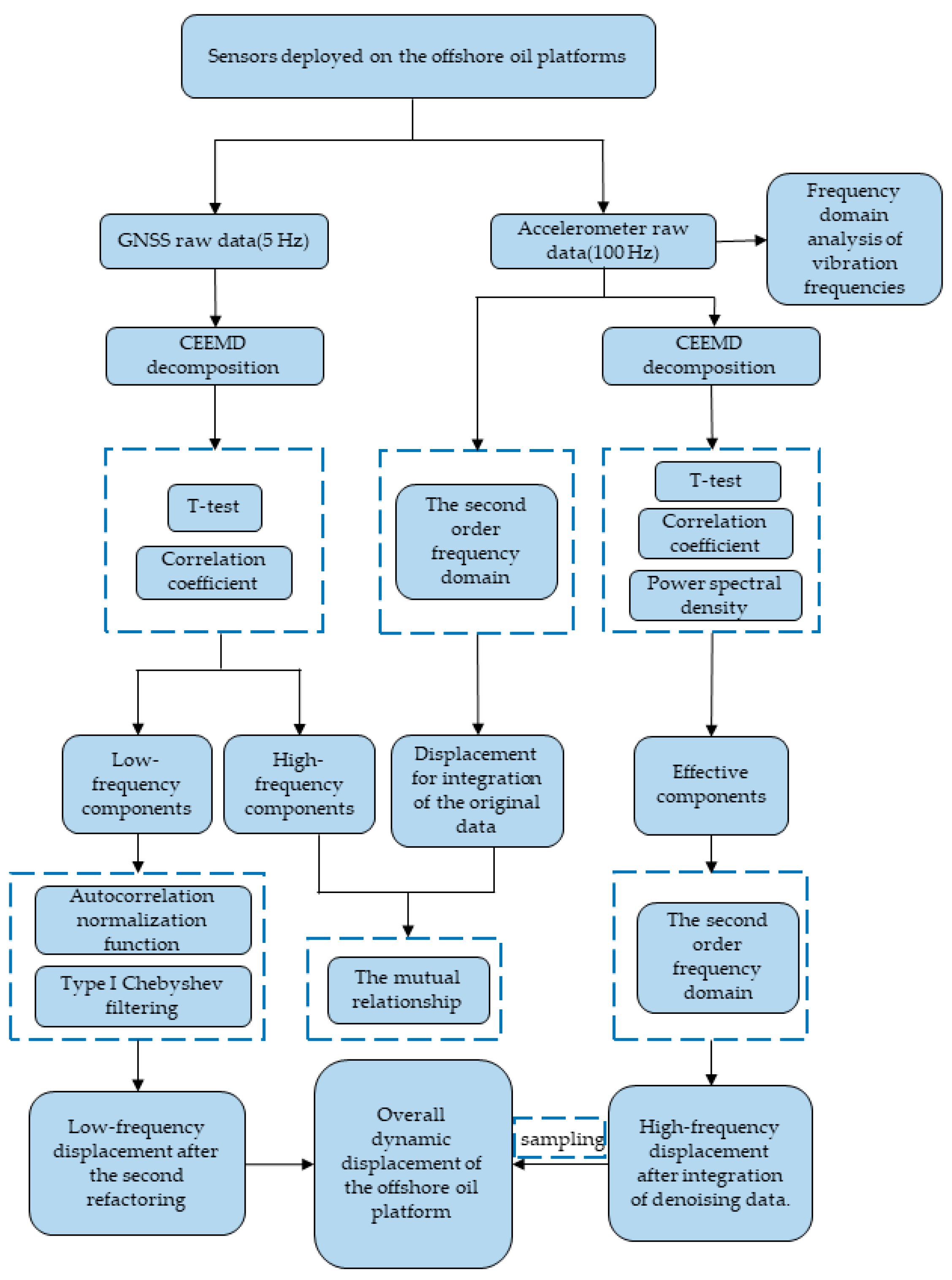
3.1. Overall Displacement Reconfiguration Process

The monitored GNSS data and acceleration data were processed based on CEEMD–Chebyshev filtering in the following steps: (1) GNSS data were deconstructed using the CEEMD approach, which involved the extraction of low-frequency components from GNSS monitoring databases using a combination of the t-test and correlation coefficient; (2) Chebyshev filtering of IMF components, which accounted for a relatively high proportion of noise in low-frequency information, and summing with the unprocessed IMF components yielded the low-frequency dynamic displacement of the platform following second noise reduction. (3) We screened the acceleration data for useful information components based on t-test and power spectral density and integrated them into the frequency domain to obtain the high-frequency dynamic displacement of the platform. (4) Finally, the extracted GNSS low-frequency displacement was combined with the integrated high-frequency dynamic displacement to form the overall dynamic displacement of the platform through data sampling. Figure 1 depicts the flow chart for the overall displacement reconstruction in this paper.

3.2. Data Processing

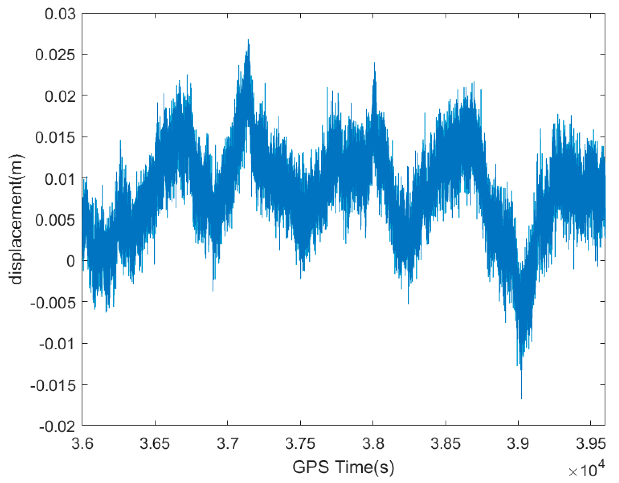
3.2.1. Introduction to the Raw Data

The monitoring experiment was carried out using both GNSS (sampling frequency 5 Hz) and a Mti300 Micro-Electro-Mechanical System inertial measurement unit (MEMS IMU) (sampling frequency 100 Hz) to monitor the displacement and deformation of the platform, utilized by ship operators for dwelling. To limit the influence of strong emission sources and multi-path effects, the reference station and monitoring station were set up in an open and unobstructed area. The monitoring station was located on top of the offshore platform CB246A in the Dongying Shengli Oilfield, at a distance of about 19.4 km from the base station. The experiment was conducted on 1 December 2019 on the offshore platform CB246A in the Dongying Shengli Oilfield, with a wind force of about four. The dynamic response of the platform in the marine environment was continuously acquired using a GNSS receiver and accelerometer.
The accelerometer used in the experiment can provide high-precision nine-axis acceleration data, gyroscopic data, and magnetometer data in both vibration and non-uniform magnetic field environments. The collected data were first converted to coordinates using suitable mathematical methods; respectively, GNSS data were converted from an Earth-Centered, Earth-Fixed coordinate system to a station coordinate system, and acceleration data were converted from a carrier coordinate system to a station coordinate system. An hour (GPS time of 36,000–39,600 s) of simultaneous monitoring data in the north direction of the intercepted plane was processed and analyzed, and the GNSS and accelerometer raw data were as shown in Figure 2 and Figure 3.

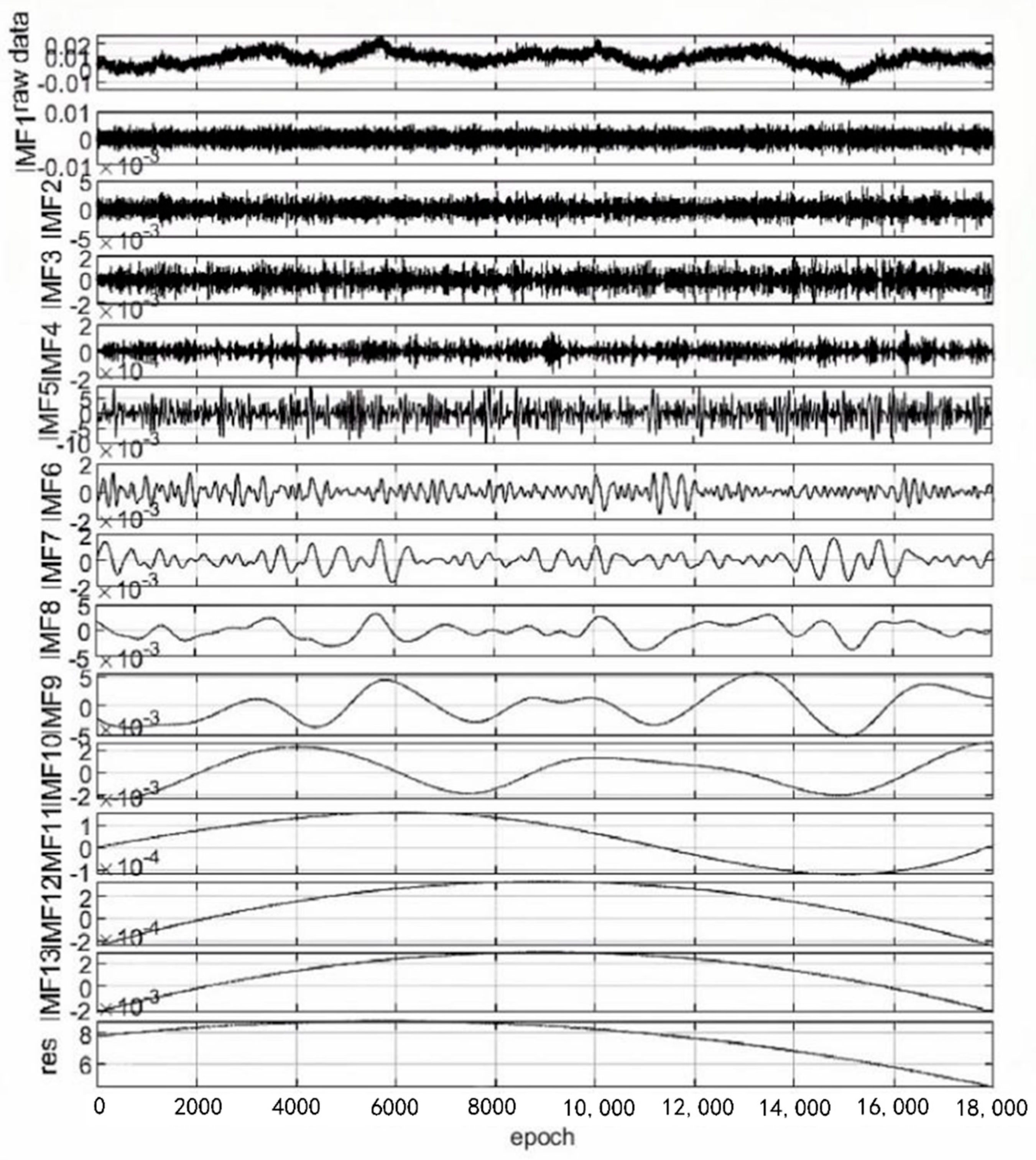
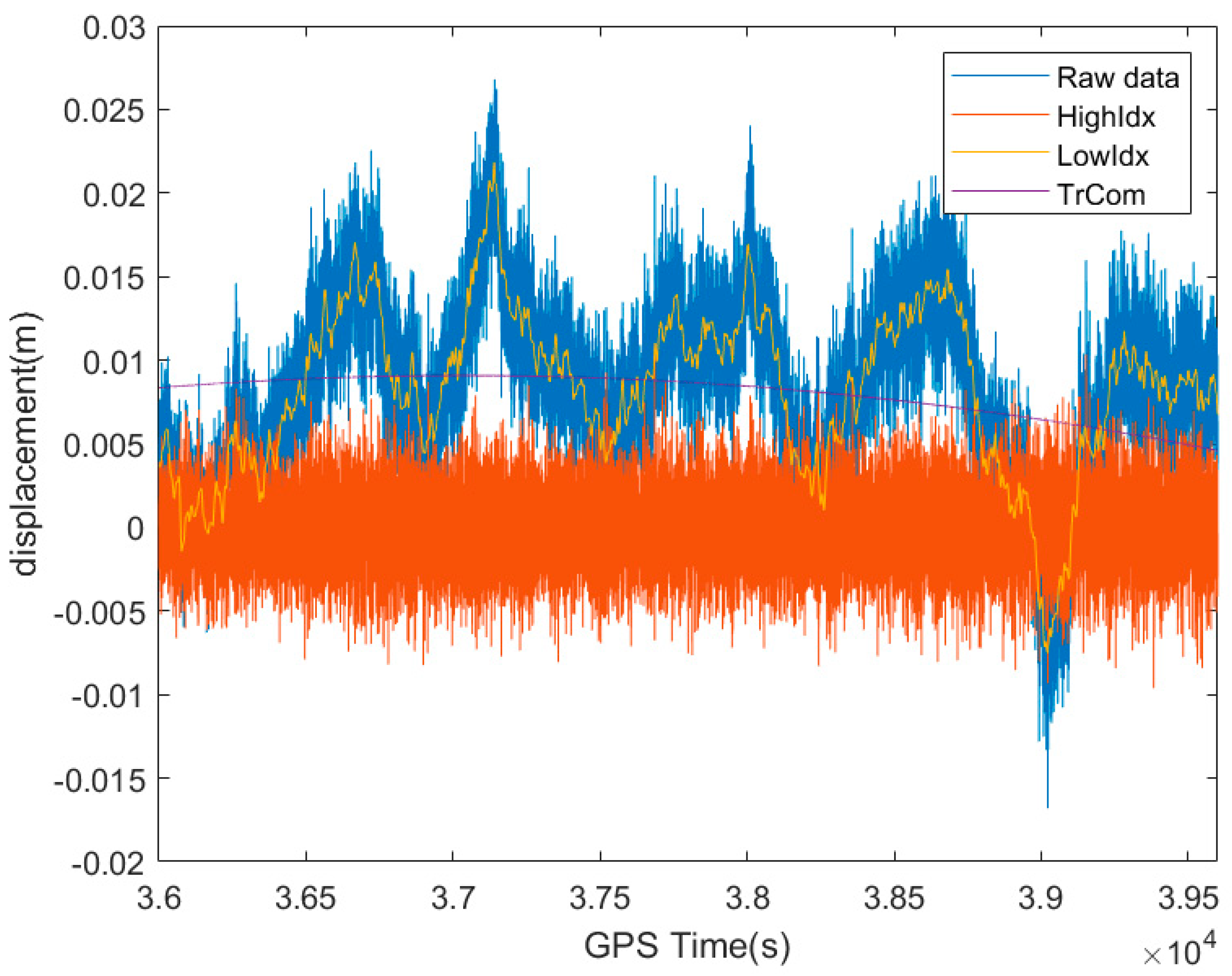
3.2.2. Processing and Analysis of GNSS Data

In the marine environment, owing to the effects of the stronger multipath than on land [16], the multipath error was more severe, there were several noise sources, and the true dynamic displacement of the platform was contaminated to some extent [29]. As shown in Figure 2, the GNSS short baseline solution results contained random noise and multi-path error effects, and the original maximum amplitude of the northward displacement of the platform obtained using GNSS was 26.79 mm. The noise-contaminated monitoring data required hybrid filtering for denoising processing in order to remove the noise that caused interference in the analysis and to extract the low-frequency components of the signal as much as possible. The procedure was as follows.
Firstly, the original GNSS data of the platform was deconstructed by CEEMD, which further decomposed the GNSS signal into IMF components distributed from high frequency to low frequency. Then the ratio of additional noise standard deviation to the original standard deviation was set as 0.2 and added to 100 groups of complementary and independent identically distributed white noise for averaging. The decomposition results are shown in Figure 4, from which it can be intuitively seen that the GNSS signal was deconstructed into different frequency (13 IMF components, and 1 trend term) residual components. Therefore, a particular technique was required to distinguish the noise component from the effective component.
In order to extract the effective information from the signal and remove the noisy IMF components, the t-test method was used to distinguish the high-frequency components from the low-frequency components. Additionally, the IMF components used to reconstruct the signal were selected by analyzing the correlation coefficients between each component and the original signal. The IMF component must conform to the local symmetry of the upper and lower envelopes with respect to the timeline. For high-frequency IMF components, several signal peaks were connected to produce the upper and lower envelopes of the components, so the symmetry of the envelopes was equivalent to the basic symmetry of the IMF component data. The average value of the data tended to be close to zero. For low-frequency IMF components with long signal periods, a small number of peaks were interpolated to obtain the envelopes, and the trend of the envelopes deviated from that of the original signal, so the signal components were not necessarily symmetrical or even distant. At this stage, it was difficult to confirm that the mean value of the IMF components was zero; hence, the t-test was used to classify the IMF components [30]. The test procedure was as follows: Sum the first m IMFs together as index m, calculate the mean of indexes 1 through 14, then conduct a t-test to determine whether the mean is significantly different from 0. Given a significance level of 0.05, the p-value is the probability that the test statistic in the t-test is as extreme or more extreme than the value observed under the original hypothesis [31]. If the p-value exceeds the significance level of 0.05, the original hypothesis is accepted. The P1 values for each index are listed in Table 1, whereas the results of solving the correlation coefficient between each IMF component and the original signal are listed in Table 2. R1 represents the correlation coefficient between the two variables, with a higher value indicating a better correlation between each IMF component and the original signal.
The data in Table 1 indicate that the test result was significantly less than 0.05 at index 7, indicating that the index mean was significantly different from 0 after adding the IMF7; therefore, the t-test classified IMF7 and its subsequent components as low-frequency components, with correlation coefficients higher at IMF8, IMF9, and IMF10. Combined with the R1 values in Table 2, IMF1-IMF6 were selected as high-frequency components and IMF7-IMF14 as the low-frequency components. The selected components were reconstructed individually to obtain the high-frequency and low-frequency features of the GNSS data. The displacement amplitude signals after the first refactoring are shown in Figure 5. The high-frequency features, HighIdx in Figure 5, were a mixture of random noise, multi-path errors, and the high-frequency displacement part of the platform. The low-frequency features, LowIdx in Figure 5, significantly reduced the impact of noise and preserved more complete and effective information than the original data, and the correlation between the two was 0.9236. However, simply adding up the low-frequency components does not ensure the integrity of denoising, and a second denoising process was required for some of the low-frequency components. The trending term, TrCom in Figure 5, represented by the last residual component of the decomposition, represents the divergence of the platform displacement signal from the baseline during that period.
The autocorrelation normalization function of the signal attained a peak at the zero point, and at other points, the value of the noise signal tended to zero. The value of the useful signal usually varies with time [32]. In the second filtering denoising process of the low-frequency IMF components, the autocorrelation characteristics of the signal were retrieved. Figure 6 illustrates the autocorrelation normalization function of each IMF component in the extracted low-frequency reconstructed signal. It can be seen from the figure that the IMF7 component still contained more noise, so the IMF7 component was subjected to a type I Chebyshev filtering process and then reconstructed with the remaining IMF components, and the trend term was summed to obtain the final GNSS dynamic displacement, as shown in Figure 7. The comparison of the low-frequency displacement amplitude of GNSS data after the first refactoring and the second refactoring is also visible in Figure 7. This indicated that the CEEMD–Chebyshev hybrid filtering reduced the high-frequency noise in the monitoring data while preserving the effective low-frequency components.

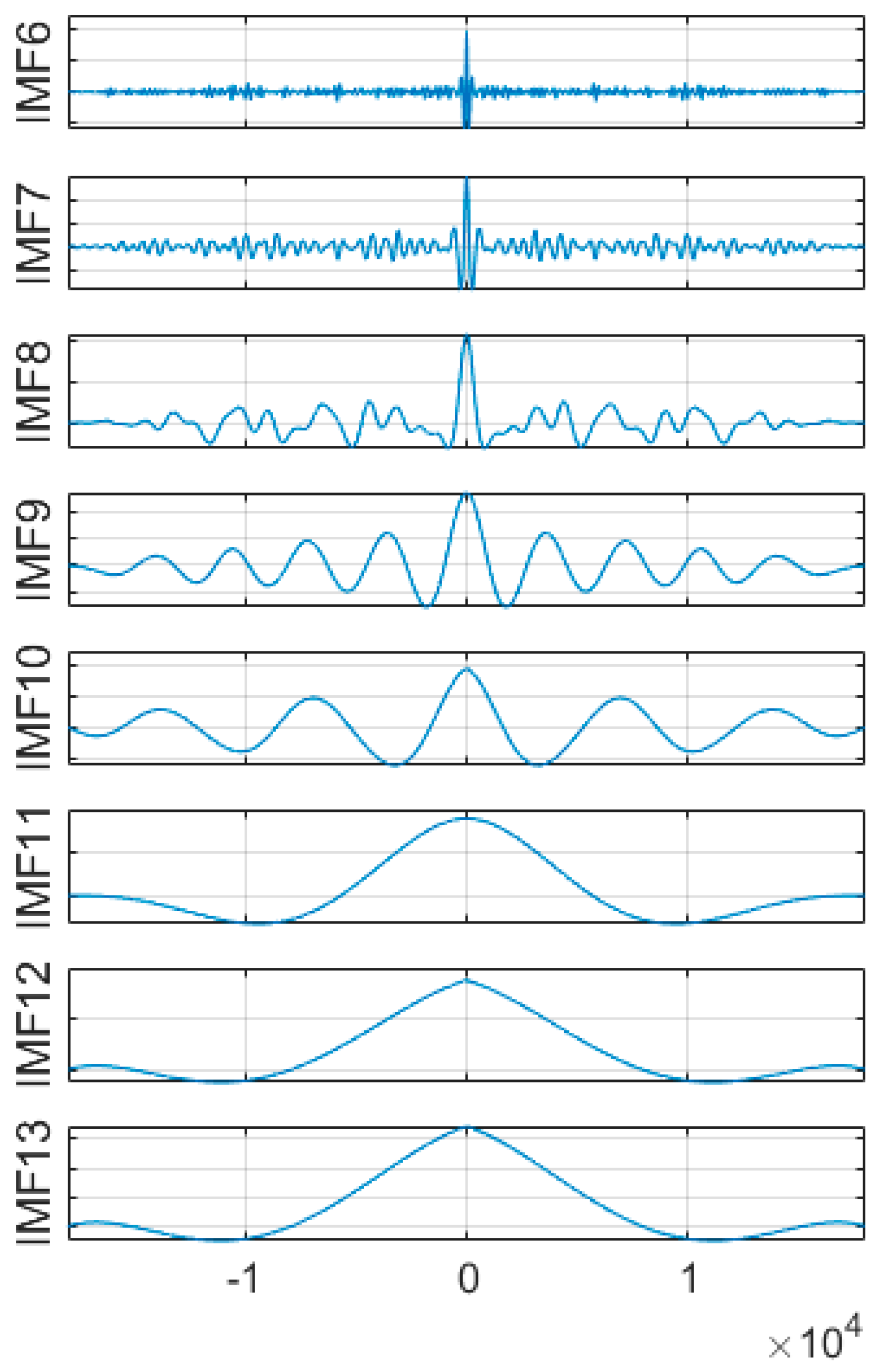
3.2.3. Processing and Analysis of Acceleration Data

An accelerometer is commonly used for structural response monitoring under external loading conditions and has the advantage of high sampling rates and easy identification of high-frequency vibrations of the structure. However, it is not sensitive to the identification of low-frequency vibrations [33]. The acceleration data was intercepted for the same period of 1 h as GNSS monitoring data, to achieve the overall displacement refactoring. The acceleration monitoring signal was initially studied in the frequency domain using FFT to process the monitoring data, finding the vibration frequencies of the platform structure. To better extract the spectral characteristics of each frequency band, the monitoring data were detrended to remove the direct current component of the signal and the amplitude was calculated logarithmically to observe the periodic signal masked by the low amplitude noise. Figure 8 shows a plot of the power spectral density of the acceleration signal. It can be observed that the power spectral density plot identifies the first three order modal frequencies of the platform in the 0–2 Hz range, i.e., the three peaks corresponding to the plot: 0.8743, 0.9087, and 0.9993 Hz.
Furthermore, the time domain characteristics of the acceleration data were analyzed, to verify that the acceleration monitoring data comprised the high-frequency vibration part of the platform. The original acceleration data was firstly integrated with the second frequency domain. The comparison of GNSS high-frequency displacements with the displacement for integration of the original acceleration is shown in Figure 9. The displacement of GNSS high-frequency reconstruction overlapped with the second frequency domain integral displacement of the original acceleration. The mutual correlation function is a correlation analysis function that describes the degree of correlation or dependence between two sets of signals. The mutual relationship number was 0.8916, and the GNSS data could not filter the high-frequency component further. Therefore, the initial acceleration data could be filtered and denoised, followed by frequency domain integration processing to derive the high-frequency displacement of the platform.
As depicted in Figure 3, the acceleration time curve recorded using the MEMS IMU had many prominent sections owing to the influence of random noise. A hybrid filtering method was used to remove the insensitive low-frequency components and to obtain the true acceleration monitoring value. The original accelerometer monitoring signal was first deconstructed into 17 IMF components and a trend term by CEEMD. The CEEMD decomposition results are shown on Figure 10a, and the corresponding power spectral density functions for each order of IMF components are shown on Figure 10b. The t-test was carried out along the same lines as for the GNSS data, and the obtained P2 values for each index are listed in Table 3. The test result was significantly less than 0.05 at index 9; hence, the high-frequency component t-test results were IMF1-IMF8 and the low-frequency component t-test results were IMF9-IMF18. The results of calculating the correlation coefficient R2 between each IMF component and the raw acceleration monitoring data are presented in Table 4.
Observing the spectrum corresponding to each IMF component on the right side of Figure 10, it is evident that the 8th order components IMF1, IMF2, IMF3, IMF4, IMF5, IMF6, IMF7, and IMF8 contain frequency information. Combining the results of the t-test and the correlation coefficients between each component and the original data in Table 4, the new acceleration data was finally obtained by selecting the IMF1-IMF8 refactoring, which was equivalent to high-pass filter discarding the low-frequency components of IMF9-IMF18 to obtain useful information components. The IMF1 and IMF2 components with larger correlation coefficients were then filtered by the Chebyshev filter to obtain the final denoising acceleration time curve, and the noise-reduced acceleration data were integrated with the quadratic frequency domain to obtain the high-frequency displacement of the platform vibration, as shown in Figure 11. Compared with the second integral displacement of the original acceleration monitoring data, the amplitude of the refactored signal after hybrid filtering denoising was smaller with a less prominent portion. This reflected the high-frequency features of the platform more accurately.

3.2.4. Overall Displacement Reconfiguration

The acceleration quadratic integral displacement was sampled so that its frequency matched that of the extracted GNSS low-frequency displacement. Figure 12 shows the overall dynamic displacement amplitude of the offshore oil platform. The correlation coefficient between the reconstructed overall displacement and the original GNSS monitoring data was 0.8576, which was high and over 0.85. The random noise and multi-path error were also reduced to a large extent, which reflected the platform structure vibration displacement more effectively and accurately, allowing it to be used for the dynamic deformation monitoring of offshore oil platforms.
In this paper, the proposed CEEMD–Chebyshev hybrid filter was used to reduce noise in GNSS and acceleration data, respectively. The effective components were selected using a combination of the t-test and the correlation coefficient, and the overall dynamic displacement of the platform was obtained by reconstructing the corrected high and low-frequency displacements, which compensated for the shortcomings of using the two types of sensor data separately. There are also certain limitations: first, in data monitoring, the sensitivity of GNSS sensor monitoring needs to be improved; second, in data processing, the overall displacement is a simple sum of low-frequency displacement and high-frequency displacement. It will be necessary to consider in the next step how to fuse the displacements obtained by the two sensors with the Kalman filtering process.

4. Conclusions

The monitoring of dynamic deformation is one of the crucial factors to ensure the safe operation of offshore oil platforms. In this paper, the overall dynamic displacement of the platform was reconstructed based on GNSS and acceleration data for the same time period. The following conclusions were drawn based on the processing and analysis of the measured data:
(1)
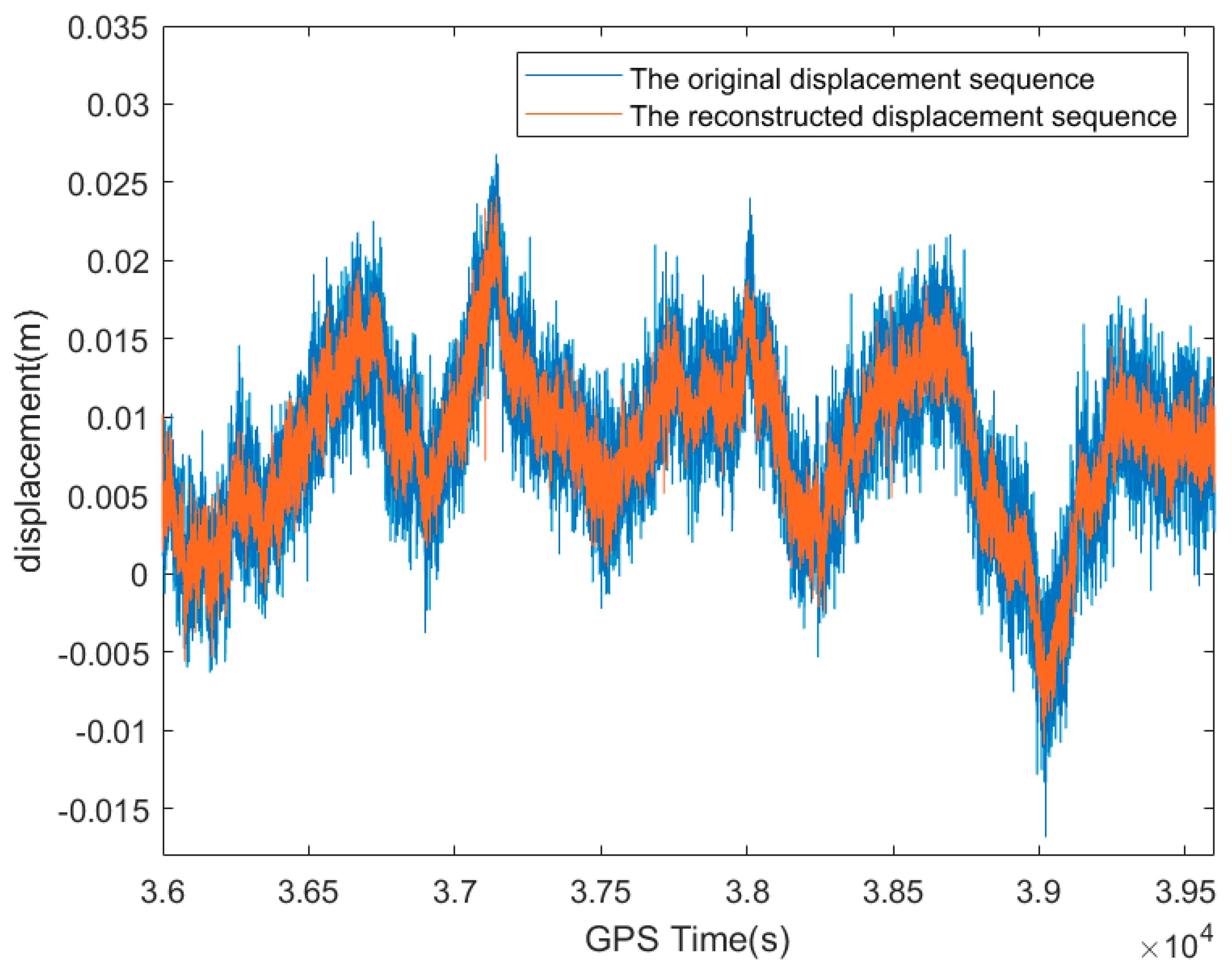
Based on the selection principles of the t-test and correlation coefficients, the CEEMD–Chebyshev hybrid filter was capable of removing the high-frequency component of the GNSS signal and reducing the noisy part of the low-frequency component, achieving effective extraction of the low-frequency displacement. The maximum displacement amplitude was reduced from 26.79 to 21.22 mm, and the correlation after denoising was 0.8860, with a high degree of correlation.
(2)
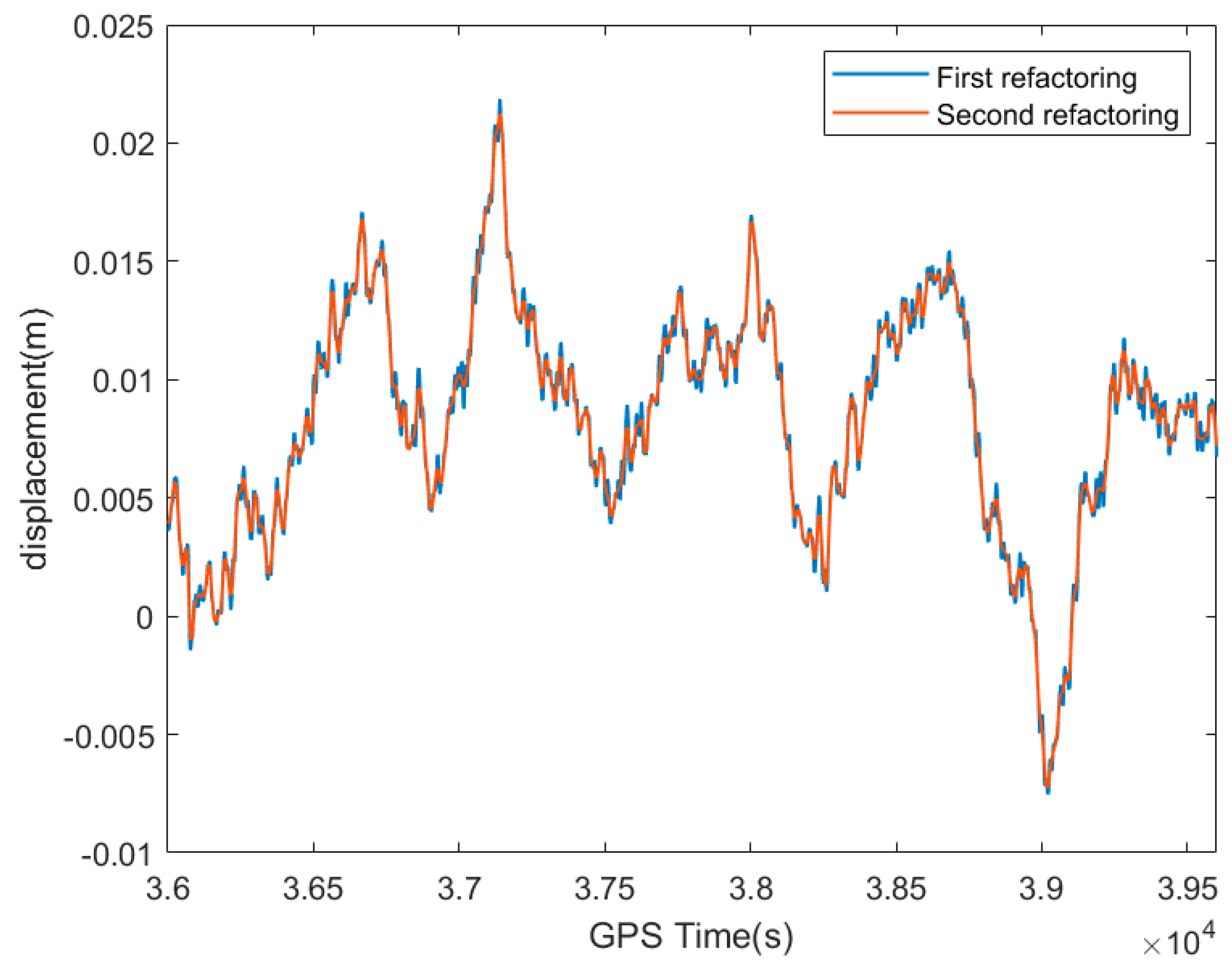
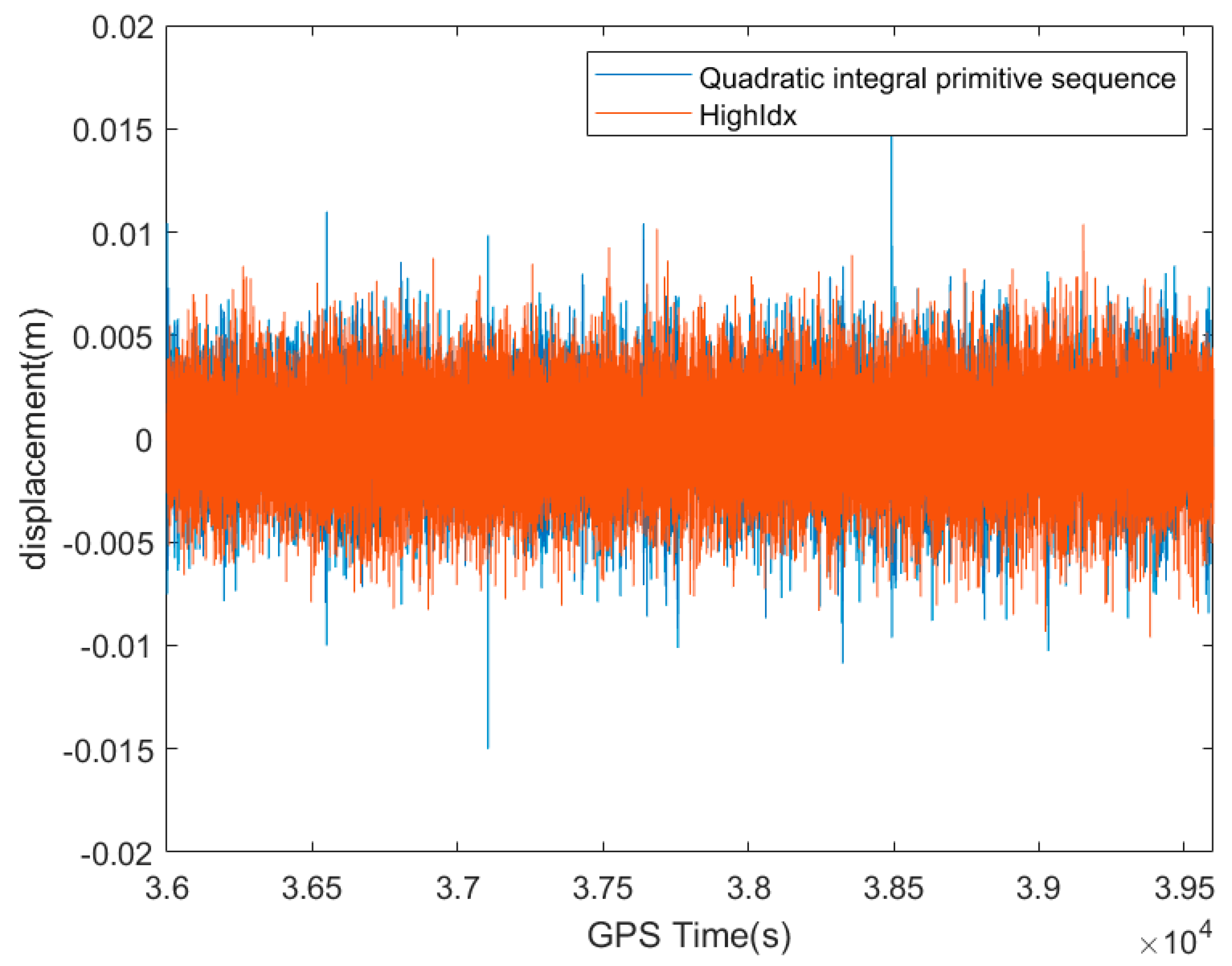
The integrated displacement of the accelerometer coincided with the high-frequency displacement monitored by GNSS, and the feasibility study indicated that the accelerometer can monitor the high-frequency vibration information of the platform. In addition, the method of frequency domain integration can avoid the influence of the integration trend term to obtain the partial displacement information of the platform.
(3)
The hybrid filter was also suitable for the processing of acceleration data when combined with power spectrum identification to filter the appropriate components to reconstruct the acceleration data and frequency domain integration to obtain the high-frequency dynamic displacement of the platform to millimeter precision.
(4)
Integrating low-frequency components from GNSS with high-frequency components from accelerometers yielded the global dynamic displacement. The correlation coefficient with the original GNSS monitoring data was 0.8576, and the signal correlation after denoising and refactoring was greater than 85%, retaining important information components and providing a significant foundation for structural health monitoring of offshore oil platforms. The integrated GNSS and accelerometer monitoring technique has certain practicality and reliability in monitoring the dynamic displacement of offshore oil platforms.

Author Contributions

Conceptualization, S.Y., C.X. and J.M.; methodology, S.Y., C.X., S.G. and J.M.; software, S.Y.; validation, S.Y.; formal analysis, S.Y.; investigation, S.Y. and C.X.; resources, S.Y., C.X. and J.M.; data curation, S.Y. and C.X.; writing—original draft preparation, S.Y.; writing—review and editing, S.Y., C.X., S.G. and J.M.; visualization, S.Y.; supervision, C.X., S.G. and J.M.; project administration, S.Y., C.X., S.G. and J.M.; funding acquisition, C.X., S.G. and J.M. All authors have read and agreed to the published version of the manuscript.

Funding

This work was supported by the National Key Research and Development Program of China (2021YFC3000504), the Fundamental Research Funds of CASM (AR2214) and the National Natural Science Foundation of China (41930535).

Institutional Review Board Statement

Not applicable.

Informed Consent Statement

Not applicable.

Data Availability Statement

Not applicable.

Acknowledgments

We would like to thank the professional reviewers and the editors.

Conflicts of Interest

The authors declare no conflict of interest.

References

  1. Liu, K.; Zhou, S.S. Safety design analysis for online monitoring of critical equipment failures on offshore oil rigs. Chem. Saf. Environ. 2022, 35, 21–24. [Google Scholar]
  2. Li, D.; Lyu, B.C.; Wu, W.H.; Li, H. Status and prospect of offshore platform on-site monitoring technology. China Offshore Oil Gas 2022, 34, 165–179. [Google Scholar]
  3. Sun, L. The Applied Research Based on Wavelet Analysis in Bridge Health Monitoring. Ph.D. Thesis, Chang’an University, Xi’an, China, 2012. [Google Scholar]
  4. Zhong, P.; Ding, X.L.; Zheng, D.W.; Chen, W.; Xu, Y.L. Filter-based GPS structural vibration monitoring methods and comparison of their performances. Acta Geod. Cartogr. Sin. 2007, 36, 31–36, 42. [Google Scholar]
  5. Chen, D.Z.; Ye, S.R.; Liu, Y.Y.; Liu, Z. Applied analysis of GPS multipath errors based on observation domain. Geomat. Inf. Sci. Wuhan Univ. 2014, 39, 147–151. [Google Scholar] [CrossRef]
  6. Qing, C.B. Study on Structural Vibration Frequencies of Bridges Based on GPS and Accelerometer. Master’s Thesis, China University of Mining and Technology, Xuzhou, China, 2016. [Google Scholar]
  7. Han, H.Z.; Wang, J.; Meng, X.L. Reconstruction of bridge dynamics using integrated GPS and accelerometer. J. China Univ. Min. Technol. 2015, 44, 549–556. [Google Scholar] [CrossRef]
  8. Roberts, G.W.; Meng, X.L.; Dodson, A.H. Integrating a global positioning system and accelerometers to monitor the deflection of Bridges. J. Surv. Eng. 2004, 130, 65–72. [Google Scholar] [CrossRef]
  9. Brownjohn, J.; Rizos, C.; Tan, G.H.; Pan, T.C. Real-time long-term monitoring of static and dynamic displacements of an office tower, combining RTK GPS and accelerometer data. J. Beiträge Zum Ausländischen Offentl. Recht Völkerrecht 2004, 118, 3305–3315. [Google Scholar]
  10. Dai, W.J.; Wu, X.X.; Luo, F.X. Integration of GPS and accelerometer for high building vibration monitoring. J. Vib. Shock 2011, 30, 223–226, 249. [Google Scholar] [CrossRef]
  11. Yu, J.Y. GNSS and RTS Technologies Based Structural Dynamic Deformation Monitoring of Bridges. Ph.D. Thesis, Hunan University, Changsha, China, 2015. [Google Scholar]
  12. Li, W.; Wang, J.; Liu, F.; Liu, X. Research on vibration monitoring model of GNSS/accelerometer based on EMD. J. Geod. Geodyn. 2021, 41, 1306–1311. [Google Scholar] [CrossRef]
  13. Zhang, L.N. Summary of time-frequency analysis method of digital signal processing. Inf. Technol. 2013, 37, 26–28. [Google Scholar] [CrossRef]
  14. Li, S.M.; Guo, H.D.; Li, D.R. Review of vibration signal processing methods. Chin. J. Sci. Instrum. 2013, 34, 1907–1915. [Google Scholar] [CrossRef]
  15. Yu, X.; Dong, F.; Ding, E.J.; Wu, S.P.; Fan, C.Y. Rolling bearing fault diagnosis using modified LFDA and EMD with sensitive feature selection. IEEE Access 2018, 6, 3715–3730. [Google Scholar] [CrossRef]
  16. Xiong, B.; Chen, W.; Zhai, J.S.; Han, L. Dynamic deformation monitoring and the data processing of offshore platform piles based on GNSS RTK technology. Bull. Surv. Mapp. 2019, 102–105. [Google Scholar] [CrossRef]
  17. Xu, R.; Bai, Y. Study on improved CEEMD–MRSVD denoising method and its application. Aeronaut. Manuf. Technol. 2022, 65, 77–82. [Google Scholar] [CrossRef]
  18. Wu, Z.S.; Wang, L.X.; Shen, Q.; Li, C.; Li, W.H. Output prediction method of HRG based on CEEMD. Syst. Eng. Electron. 2022, 1–7. Available online: http://kns.cnki.net/kcms/detail/11.2422.TN.20220117.1902.012.html (accessed on 8 August 2022).
  19. Dai, W.J.; Ding, X.L.; Zhu, J.J.; Chen, Y.Q.; Li, Z.W. EMD filter method and its application in GPS multipath. Acta Geod. Cartogr. Sin. 2006, 321–327. [Google Scholar]
  20. Zheng, J.D.; Cheng, J.S.; Yang, Y. Modified EEMD algorithm and its applications. J. Vib. Shock 2013, 32, 21–26, 46. [Google Scholar] [CrossRef]
  21. Chen, R.X.; Tang, B.P.; Ma, J.H. Adaptive de-noising method based on ensemble empirical mode decomposition for vibration signal. J. Vib. Shock 2012, 31, 82–86. [Google Scholar] [CrossRef]
  22. Wu, X.T.; Yang, M.; Yuan, X.H.; Gong, T.K. Bearing fault diagnosis using EEMD and improved morphological filtering method based on kurtosis criterion. J. Vib. Shock 2015, 34, 38–44. [Google Scholar] [CrossRef]
  23. Ding, Y.; Xu, D.H.; Cao, L.H.; Guan, X.R. Applicability of the LSTM and ARIMA model in drought prediction based on CEEMD: A case study of Xinjiang. Arid. Zone Res. 2022, 39, 734–744. [Google Scholar] [CrossRef]
  24. Tian, S.J. Design and Research of X-Band SIW Generalized Chebyshev Super Structure Filter. Master’s Thesis, School of Electronic Science and Engineering, Chengdu, China, 2020. [Google Scholar]
  25. Liu, X.; Wang, J.; Li, W. A time-frequency extraction model of structural vibration combining VMD and HHT. Geomat. Inf. Sci. Wuhan Univ. 2021, 46, 1686–1692. [Google Scholar] [CrossRef]
  26. Zhang, X.F. Analysis in Dynamic Deformation of Long Span Bridges Based on RTK-GNSS and Accelerometer Technology. Master’s Thesis, Tianjin University, Tianjin, China, 2019. [Google Scholar] [CrossRef]
  27. Fang, X.J.; Zu, H.B.; Xiong, Z.Q.; Zhang, K.F.; Gu, H.Y.; Xie, Y.C. Experimental study on flow-induced vibration of multi-span tube bundle with tube support plate. At. Energy Sci. Technol. 2017, 51, 1379–1386. [Google Scholar]
  28. Wang, Z.Y.; Wu, X.Q.; Wang, X.J.; Zhang, Y.H. Spatio-temporal evolution of mariculture in the Yellow River Delta and its impact on tidal flat wetland resources. J. Agric. Resour. Environ. 2022, 1–16. [Google Scholar] [CrossRef]
  29. Xiong, C.B.; Chen, W.; Wang, M.; Xiong, A.C.; Han, L.; Yu, L.N. Horizontal displacement monitoring of pile leg structure of offshore platform by RTK-GNSS. J. Tianjin Univ. Sci. Technol. 2021, 54, 781–789. [Google Scholar]
  30. Qi, S.Z.; Zhao, X.; Tan, X.J. A study on the formation mechanism of Chinese carbon market price based on EEMD model. Wuhan Univ. J. Philos. Soc. Sci. 2015, 68, 56–65. [Google Scholar] [CrossRef]
  31. Yan, H.N.; Dai, W.J.; Wen, Y.X. A method of processing GNSS displacement time series with t-test and characteristic function. Sci. Surv. Mapp. 2022, 1–9. Available online: http://kns.cnki.net/kcms/detail/11.4415.P.20220713.1845.002.html (accessed on 8 August 2022).
  32. Zhang, Y.H.; Wang, X.H.; Guo, L.; Zhang, S.H. Partial discharge detection for GIS based on normalized autocorrelation function and similar wavelet soft threshold. High Volt. Appar. 2018, 54, 17–24. [Google Scholar] [CrossRef]
  33. Wang, Y.R.; Huang, S.X.; Kuang, C.L. Fusion of GNSS and accelerometer monitoring data for dynamic monitoring of high-rise buildings. Bull. Surv. Mapp. 2019, 14–19. [Google Scholar] [CrossRef]
Figure 1. The flow chart for the overall displacement reconstruction.
Sustainability 14 10521 g001
Figure 2. An hour (GPS time of 36,000–39,600 s) of monitoring GNSS raw data in the north direction.
Sustainability 14 10521 g002
Figure 3. An hour (GPS time of 36,000–39,600 s) of monitoring acceleration raw data in the north direction.
Sustainability 14 10521 g003
Figure 4. CEEMD decomposition results of GNSS data.
Sustainability 14 10521 g004
Figure 5. Displacement amplitude of GNSS data after the first refactoring.
Sustainability 14 10521 g005
Figure 6. The autocorrelation normalization function of each IMF component in the reconstructed signal.
Sustainability 14 10521 g006
Figure 7. Comparison of the low-frequency displacement amplitude of GNSS data after the first refactoring and the second refactoring.
Sustainability 14 10521 g007
Figure 8. Power spectral density plot of the acceleration monitoring signal.
Sustainability 14 10521 g008
Figure 9. Comparison of GNSS high-frequency displacements with the displacement for integration of the original acceleration.
Sustainability 14 10521 g009
Figure 10. (a) CEEMD decomposition results of acceleration data and (b) the corresponding power spectral density functions for each order of IMF components.
Sustainability 14 10521 g010
Figure 11. High-frequency displacement amplitude of platform vibration after integration of denoising acceleration.
Sustainability 14 10521 g011
Figure 12. Overall dynamic displacement of the offshore oil platform.
Sustainability 14 10521 g012
Table 1. The p1 value of the t-test for each index.
IndexP1IndexP1
index 10.6461index 80.0001
index 20.8844index 92.00 × 10⁻⁶
index 30.8377index 105.94 × 10⁻¹⁶
index 40.6491index 110
index 50.9306index 120
index 60.4012index 130
index 70.0006index 140
Table 2. Correlation coefficient R1 for each IMF and signal response.
IMF ComponentR1IMF ComponentR1
IMF10.3847IMF80.5049
IMF20.2330IMF90.7003
IMF30.1598IMF100.4714
IMF40.1185IMF110.3383
IMF50.0940IMF120.3470
IMF60.1339IMF130.3446
IMF70.2764IMF140.2485
Table 3. The p2 value of the t-test for each index.
IndexP2IndexP2
index 10.8528index 100.0009
index 20.9599index 111.03 × 10−77
index 30.8528index 121.29 × 10⁻⁶
index 40.9364index 131.81 × 10−72
index 50.9196index 140.0002
index 60.7604index 153.14 × 10⁻⁶
index 70.7089index 160
index 80.2409index 170
index 90.0001index 180
Table 4. Correlation coefficient R2 for each IMF and signal response.
IMF ComponentR2IMF ComponentR2
IMF10.7790IMF100.0018
IMF20.4726IMF110.0019
IMF30.3157IMF120.0015
IMF40.2461IMF130.0010
IMF50.1775IMF140.0012
IMF60.2029IMF150.0013
IMF70.1639IMF160.0011
IMF80.0844IMF170.0021
IMF90.0032IMF180.0022
Publisher’s Note: MDPI stays neutral with regard to jurisdictional claims in published maps and institutional affiliations.

