Study on Stability of Anchored Slope under Static Load with Weak Interlayer

Abstract

To study the stability characteristics of a rock slope with a weak interlayer, a test of the anchor frame slope was designed in this paper. The analysis model was established with FLAC^3D, and the development law of safety factor, deformation, axial anchor force, soil pressure and maximum shear strain increment of the slope, and the supporting effect of frame anchor cable were obtained by grading loading. The research showed that the supporting effect of frame anchor cable support on the slope was remarkable, and the influence of slope vertical load on the slope safety factor was evident. The lateral deformation mode of the slope surface was large up and down, and minor in the middle. The weak intercalated layer blocked the internal diffusion of the settlement. The failure trend of slope was sliding along the weak interlayer and collapse occurred below the loading zone, and the final failure mode is wedge failure. The peak value of maximum shear strain increment was developed along the weak interlayer, and a shear strain mutation zone was formed inside the slope. It could be considered that the weak interlayer was the potential sliding surface of the slope.

1. Introduction

Landslides are a serious geological disaster due to their rapid occurrence and extensive hazards [1,2,3]. Landslides are more common in rocky slopes, mainly because they contain a large number of weak interlayers, which are weak in elastic modulus and strength and often play a decisive role in the failure of slopes under external load [4,5,6]. Therefore, enough attention should be paid to the slope with a weak interlayer, and timely treatment and protection should be carried out. There are many methods for slope support, among which the most commonly used include the prestressed anchor cable with frame beam and soil nail. Soil nailing reinforcement is a kind of shallow slope reinforcement technique, which is suitable for soft rock slopes or soil slopes, and the research has obtained rich results [7,8]. When the slope is high and the potential fracture surface of the slope is deep, the prestressed anchor cable is a better method for deep reinforcement. The pre-stressed anchor cables with frame beam structure are a commonly used support structure form. The structure adopts prestress on the prestressed anchor cable to closely connect the potential sliding rock mass and stable rock mass as a whole, increasing the sliding resistance of rock and soil mass at all levels, and effectively connecting each anchor cable to the whole through the slope frame beam. This forms a reinforcement system from the surface to the inside, and then achieves the purpose of preventing overall slope instability [9,10,11,12].

The existence of the weak interlayer of the rock slope changes its mechanical characteristics. Xu et al. [13] analyzed creep characteristics and long-term strength of weak interlayers through the triple shear creep test, and concluded that the creep characteristics of a weak interlayer would weaken slope stability. Li et al. [14] used numerical simulation to analyze the controlling effect of multilayer weak interlayer on slope stability and its failure mode. Zhang et al. [15] systematically studied creep deformation behavior and stated that the progressive degradation of predominant discontinuity from primary soft rock stratum to weak interlayer is the fundamental which provides the possibility of kinematic release.

Great progress has been made in the study of the anchor frame slope. Lin et al. [16] studied the seismic response of the sheet-pile wall with an anchoring frame beam through the shaking table test and a numerical simulation. Zhang et al. [17] combined the anchor cable and lattice beam, and this was remarkable for stabilizing the middle and lower parts of the potential sliding body by the large-scale shaking table test. Based on the dynamic centrifuge test results, Yan et al. [18] studied the seismic behavior of a special slope under the interaction with a WIL. Gang et al. [5] used the Hilbert-Huang Transform marginal spectrum to study the dynamic damage development process inside the rock slope with a weak interlayer, and finally proposed the dynamic failure mode of extrusion and sliding of middle rock strata. Peng et al. [10] concluded that the installed bolt and long anchor reinforcement measures effectively kept cracks closed and maintained rock slope stability. Although much progress has been made in seismic conditions, the study of slope internal analysis needs further discussion.

Typical research methods for determining mechanical response characteristics under a slope include a model test and numerical simulation. Numerical simulation can be used for stress calculation and stability analyses of slopes, allowing for nonlinear material behavior, complex boundaries, and additional loading conditions. Wu et al. [19] used FLAC^3D software to simulate anchor frame beam reinforcement expansive soil slope to make up for the deficiency that limits equilibrium method cannot evaluate its reinforcement effect. Yang et al. [20] analyzed the reinforcement slope based on stress and displacement fields to optimize the anchor cable position and length. Yan et al. [21] proposed a slope stability evaluation method that considers the dynamic change in anchor cable axial force under seismic conditions and proved that anchor cable has a good seismic effect. In the above studies evaluating the stability of slopes, the influence of a weak interlayer in slope, especially in the anchoring slope, is ignored. Meanwhile, the evolution characteristics and action mechanism of the structural plane are still unclear.

In this paper, the scale model of anchor frame rock slope with a ¾-length weak interlayer was designed indoors. By applying a graded load to the top of the slope, the deformation of slope under the action of slope overload was tested. On the basis of experimental verification, the finite difference software FLAC^3D was used to analyze the development law of slope stress and shear strain increment. Accordingly, the failure mode of anchor frame slope with weak interlayer was revealed and provided a reference for comprehensive treatment and engineering reinforcement of slope with a weak interlayer.

2. The Model Test

2.1. Basic Test Conditions

The size of the model box used in this test was 160 cm × 100 cm × 160 cm (length × width × height), made of steel plate, steel section, tempered glass, etc. To reduce the friction of the inner wall of the model box on the structure, PTFE film was pasted on its inner wall and a layer of petroleum jelly was brushed. The test was carried out with FB-S large electro-hydraulic servo multi-channel coordinated loading system with a maximum vertical loading of 300 kN (Figure 1).

2.2. Similarity Design and Model-Making Procedure

Considering various factors, nine critical test physical quantities were selected for similarity design (

Table 1. Similarity ratio of test physical quantities.

Physical Quantity	Size	Weight	Strain	Stress	Displacement	Poisson	Friction	Cohesion	Young
Similarity ratio	1/8	1	1	1/8	1/8	1	1	1/8	1/8

), and the geometric similitude ratio was determined as 1:8 by similarity theory.

Due to the limitations of the test conditions, it is very difficult to make a complete similarity between model and prototype for all relevant physical quantities. To make the model reflect the prototype situation as much as possible, a similar model design was carried out with the key factors affecting its mechanical properties.

In this test, the rock slope was made of river sand, plaster, and water at a ratio of 8.5:1.5:1.3. The weak intercalated layer with a thickness of 20 mm was simulated by a mixture of river sand, clay, and water, whose mass ratio was 7:3:1.3, respectively. The H59 solid copper bar, 5 mm in diameter, was used to simulate the free part of anchor cable with a length of 650 mm. The anchor cables with anchorage length of 450 mm were installed in the pre-buried PVC pipe inside the slope. The dip angle of the anchor cable was 15° and the prestress was 500 N (Figure 1). The frame beams were formed from Ultra-High-Performance Concrete (UHPC). The physical and mechanical parameters of slope components in the model test were measured by the indoor geotechnical test, as shown in

Table 2. Material parameters of the slope model.

Material	Density (kg/m3)	Young (MPa)	Poisson	Cohesion (kPa)	Friction (°)
Rock mass	2100	140	0.25	252.6	36
Weak intercalation	2000	0.6	0.25	8.7	23

.

2.3. Layout of Monitoring Points and Loading Conditions

The data to be collected in this test included horizontal displacement, vertical settlement, anchor cable axial force, and earth pressure. A total of nine axial force sensors, seven displacement meters, and five earth pressure cells were installed, and the specific positions are shown in Figure 1.

The test model was filled in 24 layers at an interval of 50 mm, and each layer was filled according to the mass calculated from the corresponding layers. After the initial leveling of the filled rock material, it was compacted from the four sides to the middle with a rammer, and the places that could not be compacted by the rammer were compacted with long wooden strips, and the height was strictly controlled when the model was filled. After the completion of filling 200 mm of bedrock, the lower end of the frame beam was supported by the wooden wedge, and the upper end was tied with iron wire, so that the angle of the frame beam was the angle of the slope, and bury the anchor solid in the side slope according to the specified inclination and position.

The weak intercalated layer area shall be filled in sections according to the proportion of sand, with one section for each quarter slope height. During filling, the rock slope was filled to the height of the structural surface, and the slope mixed sand was prepared to simulate the thickness of 20 mm weak intercalated layer. Because the thickness of the weak intercalated layer was too thin to be poured, a similar material to the weak intercalated layer with poor fluidity was especially prepared, and the method of artificial smearing was used to make the weak intercalated layer. The remaining rock slope was filled after the weak intercalated layer was laid. During filling, use strip wood to touch the outside of the frame beam, fill the remaining rock materials, and thoroughly tamp.

After the filling of the test model was completed and the prestress of the anchor cable was no longer lost, the graded load was applied at the top of the slope, starting from 0 kPa and controlling the load increment of 100 kPa per grade. When the upper-level load was applied, after the difference between three consecutive readings of slope deformation value was not more than 0.01 mm. The monitoring values were stable, it was regarded as reaching the stability standard, and the corresponding data reading could be carried out. Then the next level load was applied until the partial damage was observed or excessive deformation was detected.

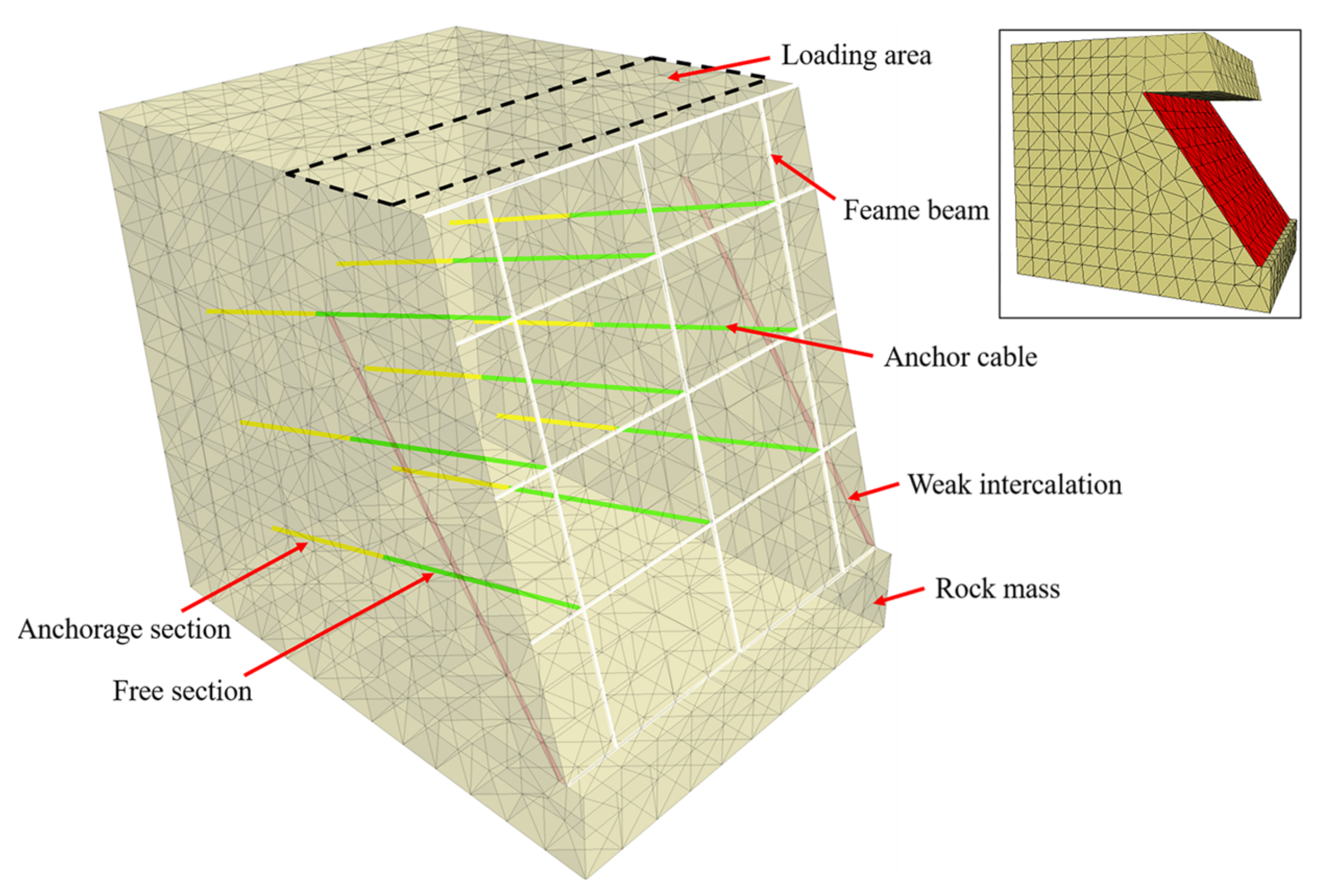
3. Numerical Simulation

The numerical model of the anchored slope with a weak interlayer was established on the FLAC^3D numerical platform according to the model test properties. FLAC^3D uses explicit Lagrangian algorithm and mixed-discrete partition technology, which can simulate the plastic failure and flow of materials very accurately, and effectively solve the problem of complex working conditions and large deformation [22,23]. The slope stratum and weak interlayer were simulated by the built-in solid element, and the anchor cable and frame beam were simulated with the cable and beam of structural element, respectively. The force transmission and interaction between the anchor cable and the frame beam were realized by setting the rigid links. The numerical model of the slope after final meshing is shown in Figure 2, which contains 7521 solid elements, 54 anchor elements, and 32 beam elements. The boundary conditions included horizontal restraints on the sides and full fixity at the base of the model. The initial state of the slope was obtained with the model set to equilibrium under gravity.

The Mohr–Coulomb constitutive model, which can better reflect the elastic-plastic properties of rock, was adopted to simulate the mechanical behavior of the slope deformation without considering the influence of pore water pressure on FLAC^3D numerical model. The relevant physical and mechanical parameters are shown in

Table 3. Mechanical parameters of the anchor frame beam.

Mechanical Parameters of the Anchor		The Parameters of the Frame Beam
Density(kg/m3)	8400	Density(kg/m3)	2500
Young (GPa)	70	Young (GPa)	9
Grout-cohesion (kPa)	100	Poisson ratio	0.3
Grout-friction (°)	30
Grout-stiffness (MPa)	1000
Grout-Perimeter (m)	0.157

.

4. Numerical Model Verification

4.1. Horizontal Displacement

Horizontal displacement is an essential basis for judging the sliding characteristics of the slope, and the recorded horizontal displacements can better reflect the deformation of the slope. Figure 3 shows the test and simulation values of horizontal displacement of slope under the action of additional loads. In the test, five monitoring positions on the slope were arranged to capture the horizontal displacement of the slope, which were designated as Points 1–5, as shown in Figure 1. Positive and negative deformation values are related to concave and uplift. In Figure 3, T represents the test results and N represents the numerical simulation results.

As can be obtained from Figure 3, the test results and simulation results of horizontal displacement at each monitoring position show good consistency in the values and the development trend, which reflects the reasonableness of the numerical simulation method. Due to the inevitable friction between the bottom beam and the bedrock at the boundary during the loading process, a certain boundary effect was caused, so the corresponding displacement value at this position (No) was small.

It can be found that the horizontal displacement increases with the additional loads, and the displacement growth rate of the top and foot of the slope increases significantly under the large slope vertical load. The horizontal displacement in the middle of the slope is the smallest, and the growth trend is relatively flat. Finally, the deformation mode of the slope surface presents an overall convex shape of the upper and lower parts are large, and the middle is small. The maximum deformation value appeared at measuring Point 1; namely the foot of the slope.

4.2. Vertical Settlement

The positions near both sides of the loading plate were selected to read the settlement on the top surface of the slope in the model test (Figure 1). Since the slope surface deformation would be caused during the slope compacting backfill and displacement meter burial, the percentage meter was zeroed out after the instrument was installed. Figure 4 shows the test and simulated values of the top surface settlement of the slope under various levels of additional loads. It can be seen that the test and simulated values show good consistency. On the whole, the test value is larger than the simulated value, which is mainly attributed to the following reasons. First of all, because the model test does not homogenize the soil layer when filling soil as in the numerical simulation, the loading process is also the process of compacting the soil layer. Second, due to the long weak intercalated layer in the test, the frame beam will not only be squeezed and rotated by the filler laterally, but also the slope body will slide along the weak intercalated layer under the action of top overload, resulting in settlement. The frame beam will rotate around the middle beam, with the top being introverted and the middle and lower parts being extroverted. Finally, when the vertical load was loaded to 300 kPa, a crack appeared on the rear edge of the loading plate and developed downward with the increase of the load, resulting in the collapse of the soil at the top of the slope. Therefore, the actual monitoring data would be larger than the simulated equilibrium data.

It can be seen from Figure 4 that the settlement on the side near the slope-free surface has immense value and rapid growth. Moreover, the maximum test value reaches 4.300 mm, and the simulation value is 2.462 mm. The significant difference between the test value and the simulation value after 400 kPa is due to the torsional deformation of the test frame beam at 400 kPa, the cracks between the frame beam and the soil at the top of the slope, and the fracture of the frame beam after 500 kPa. However, the beam structure element used in the simulation was a linear elastic material with isotropic and non-yield.

5. Results and Discussion

5.1. Factor of Safety

The safety factor (FOS) is a vital evaluation index in slope stability analysis. The slope FOS is commonly determined using limit equilibrium analysis. In this approach, the sliding mass is divided into slices, and equations of force or moment equilibrium of slices are satisfied. However, this approach does not consider the interrelationship between stress, strength, and displacement [24].

To improve the deficiency of the limit equilibrium method, Zienkiewicz et al. [25] introduced the shear strength reduction (SSR) method which was later developed by Dawson et al. [26], and Griffiths and Lane [27]. In this approach, stress-strain analysis is carried out in which shear strength is progressively reduced to bring the slope to the point of failure where numerical convergence is no longer possible. The scaling of shear strength is possible by applying a strength reduction factor (SRF) to shear strength parameters:

$${\mathrm{c}}^{\mathrm{trial}}=\frac{\mathrm{c}}{ \mathrm{SRF}}$$

(1)

$${\tan \mathsf{\phi }}^{\mathrm{trial}}=\frac{\tan \mathsf{\phi }}{\mathrm{SRF}}$$

(2)

where c^trial and φ^trial are the trial values of cohesion and friction angle for a given SRF, respectively.

At present, there are two main methods to determine the slope safety factor with the shear strength reduction. The inflection point method: calculation of slope foot displacement by reducing strength parameters of rock and soil mass. On this basis, the curve of slope foot displacement and strength reduction coefficient is drawn. It can be found that the displacement has a mutation phenomenon with the increase of reduction coefficient, and the strength reduction coefficient corresponding to the mutation point of the curve is taken as the slope safety factor. The convergence method: the slope reaches the ultimate failure state through strength reduction, and whether the calculation is convergent or not is taken as the basis of slope failure. The strength reduction coefficient corresponding to the exact convergence is the safety factor of slope stability [12]. The convergence method is influenced by certain numerical methods and has certain limitations: slope instability of the slope soil inside the plastic strain and stress level, the change and distribution of certain physical quantities has some special features, this feature will not depend on the adopted by means of numerical calculation, and the unbalanced force and the ratio of the loading at the nodes caused by more than 10⁻³ numerical convergence as the instability and failure of slope on the basis of a certain arbitrariness. At the same time, the instability criterion considers that failure occurs if there is still no convergence within a given number of iterations and convergence criteria in the nonlinear finite element calculation. Therefore, it is unreasonable to take the non-convergence of the iterative solution process as the instability criterion and the applicability is poor. Therefore, this paper adopted the inflection point method to calculate the safety factor of the slope. To reflect the characteristics of the displacement mutation and quantitative relationship, the form of the slope stability was carried out on the displacement curve fitting, and the fitting equation of the need was established.

In this paper, according to the mutation characteristics of the curve, the relationship between displacement and reduction coefficient is assumed to satisfy the hyperbolic equation. Select the form of hyperbolic equation as follows:

$$\mathsf{\delta }=\frac{\mathrm{b}+\mathrm{cK}}{1+\mathrm{aK}}$$

(3)

where a, b and c are undetermined coefficients, δ is the displacement value, and K is strength reduction factor.

Figure 5 is the fitting curve of slope foot displacement and slope safety factor under 500 kPa load. According to the conditions satisfied by the fitting equation, the reduction factor is the overall safety factor of the slope. The fitting results are shown in Figure 5. The mutation safety factor of displacement is 2.330, and the correlation coefficient R² is close to 1.

Figure 6 shows the safety factor curve with the change in slope vertical load. To analyze the influence of slope vertical load on safety factor, the difference of safety factor (Equation (4)) and the mean of the difference in safety factors (Equation (5)) are defined.

$$\mathsf{\Delta }{\mathrm{F}=\mathrm{F}}_{\mathrm{S}}^{{\mathrm{P}}_1 }{- \mathrm{F}}_{\mathrm{S}}^{{\mathrm{P}}_2}$$

(4)

$$\overline{\mathsf{\Delta }\mathrm{F} }=\frac{\mathsf{\Delta }\mathrm{F}}{5}$$

(5)

It can be seen from Figure 6 that with the increase of slope vertical loads, The degree of reduction of slope safety factor is different. When the load is 0~100 kPa, the difference value of safety factor is ΔF = 4.03 under no support condition, and the mean value of safety factor is ΔF = 10.48 under support condition. When the load is 400~500 kPa, the difference value of safety factor without support is ΔF = 0.08, and the mean value of safety factor under support is ΔF = 0.16. It can be concluded that the overall decreasing trend of safety factor is first fast and then slow. The slope supported by a frame anchor is always in a stable state. In contrast, the safety factor of the slope without a frame anchor is reduced to below 1.35 (According to the Technical code of China building slope engineering, the safety grade of slope engineering is grade 1, so the safety factor should not be less than 1.35) after loading to 100 kPa and gradually tends to be unstable, indicating that the supporting effect of a frame anchor is evident and the overall stability of the slope is ensured.

At the same time, it can be seen from Figure 6 that when the anchorage slope has no load, the safety factor is 16.592, and when a 100 kPa load is applied, the safety factor decreases rapidly to 6.177. Therefore, the load’s effect on the safety factor of the slope is pronounced. Supporting safety coefficient under the condition of no difference between the mean $\overline{\mathsf{\Delta }\mathrm{F}}$ = 1.09, supporting under the condition of safety coefficient difference mean $\overline{\mathsf{\Delta }\mathrm{F}}$ = 2.85. When the load is 0~100 kPa, the difference of safety factor is much larger than the mean value. When the load is greater than 100 kPa, the difference of safety factor is smaller than the mean value. When the load is 400~500 kPa, the difference of safety factor with or without support reaches the maximum, which is 2.69 and 1.01, respectively. When the slope vertical load is puny, the influence on the safety factor is enormous. When the slope vertical load is large, the influence on the safety factor of the slope is small, which can be verified with the axial force analyzed later. When the load on the top of the slope increases, the axial force of the anchor cable increases sharply, bearing part of the additional load on the slope and delaying the failure trend of the slope. However, the safety factor can only evaluate the overall stability of the slope, and whether the local failure occurs cannot be reflected by the safety factor. It is urgent to conduct profound research.

5.2. Anchor Axial Force

Figure 7 shows the axial force variation curve of the anchor cable under different loads, and the layout of anchor cable is also shown in Figure 7. It can be seen from Figure 7 that the axial force of anchor cable gradually increases with the increase of additional loads, and the axial force of anchor cable shows a “linear growth” trend from 0 to 300 kPa. After more than 300 kPa, the slope appears elastic-plastic coexistence, and the axial force starts to grow abruptly under the load. The growth of the internal force of anchor cables No.1 to No.3 at the top of the slope and No.7 to No.9 at the foot of the slope is the most obvious, with the maximum value reaching 2.118 kN. In contrast, the growth of the internal force of anchor cables No.4 to No.6 in the middle of the slope is relatively slow, and the slope deformation verifies. The lateral deformation of the slope top and slope toe is evident, and the axial force of the anchor cable increases, which bears more load.

At the beginning of loading, the load on the top of the slope was mainly borne by the slope soil, and the axial force of the anchor cable changed relatively slowly. When the load gradually increased to 300 kPa, the role of the anchor cable was extensively played. It begins to bear the load on the top of the slope together with the rock and soil mass, and the axial force curve begins to steepen, and the load is transferred from top to bottom. Therefore, the anchor cable at the top of the slope first bears the upper load. The rock and soil mass above the weak interlayer was continuously squeezed under the load, the deformation increased sharply, and the compressive stress at the foot of the slope continued to increase, so the bearing capacity of the anchor cable at this position was fully exerted.

Therefore, compared with the location of the broken waist, the anchor cable axial force at the top and foot of slope increases rapidly, which corroborates with the displacement and safety factor changes in the previous section, reflecting the deformation law and damage mode of the slope, where the top surface of the slope collapses locally due to the continuous action of the additional load, and the middle and bottom due to the presence of a weak internal interlayer, resulting in the reduction of the shear strength and bearing capacity of the slope body, and the dumping damage along the weak interlayer. The action of the frame anchor cable restrains the deformation of the slope body and delays the behavior of rapid damage to the slope. In the actual project, to improve the slope support strength and bearing capacity and give full play to the performance of material, the anchor cable strength design should adopt a progressive design. The design strength of the upper and lower anchor cables should be increased appropriately, and the anchor cable strength in the middle position can be reduced appropriately.

5.3. Slope Deformation

In the test, only the settlement near two sides of the loading plate was measured, which cannot fully reflect the deformation law of slope settlement. Therefore, in order to further analyze the overall deformation law of the slope under the load on the top of slope, the overall settlement of the slope will be shown by numerical simulation. Limited to space, only the deformation under the action of 500 kPa slope vertical load is given for comparison. At the same time, the settlement diagram without weak interlayer under this condition is given (Figure 8).

It can be seen from Figure 8a that without the weak interlayer, the settlement of the anchoring slope gradually diffused along the bottom of the loading plate. With the increase in depth, the settlement value became smaller, and the maximum settlement value was 1.835 mm. When there is a weak interlayer, the vertical settlement caused by additional load mainly appears directly under the loading area, with a maximum value of 2.952 mm. The settlement value decreases step by step along the bottom of the loading area. The existence of the weak interlayer makes the settlement peak concentrated above it, which significantly weakens the settlement development. Moreover, the settlement peak value is significantly greater than that of the slope without weak interlayer. Meanwhile, the slope near the loading area is affected by the diffusion of additional vertical stress, and there is an enormous settlement value. The effect of stress diffusion increases with the proximity of the loading plate.

In summary, the settlement spreads around the loading area due to no weak interlayer above the slope. After the weak interlayer’s emergence, with the peak load’s increase, the vertical settlement diffusion trend disappears, is isolated from the weak interlayer, and gradually develops downward along the top of the weak interlayer. Meanwhile, there is no obvious deformation behind the slope, which is relatively stable. Combined with the above displacement development trend, it can be seen that the presence of a weak interlayer has a significant impact on the slope. The slope initially forms a sliding zone above the weak interlayer (as shown in Figure 8b), and the gradual increase of load makes it possible for the slope to slide out from the slope foot along the weak interlayer.

Figure 9 is the displacement vector diagram of the slope under the additional load of 500 kPa. The arrow’s size and direction represent the displacement vector’s size and direction. As can be seen from Figure 9, the displacement deformations at the top and foot of the slope are evident, and the deformation values exceed 4 mm. The displacement deformation near the foot of the slope is the most obvious, and the maximum displacement also appears here, reaching 6.109 mm. The deformation in the middle is small, approaching below 4 mm. Combined with the displacement vector, it can be seen that the displacement vector of the slope is roughly parallel to the soft structural plane, showing “shear”, and the displacement vector of the slope foot shows “cut out” at the bottom. The slope has a sliding trend along the direction of the weak interlayer, and the deformation accumulates seriously at the slope toe.

Combined with the change law of displacement, it can be concluded that the existence of additional load destroys the original stress balance state of the slope, and the stress redistribution and local stress concentration occur on the slope, and the anti-sliding force of the slope is reduced, leading to local deformation and sliding.

After the vertical load is constantly applied, the stress conditions inside the slope change, resulting in uneven settlement and stress redistribution inside the slope. The deformation and failure of the slope are mainly controlled by the concentration of tensile stress at the top of the slope and the concentration of shear stress on the slope. Tensile cracks are formed at the edge of the loading zone and extend to the weak interlayer to form a potential slip surface. At the same time, the loading area is gradually transformed into the compression and shear plastic belt, which is gradually connected and extended to the lower part, and the overall deformation and failure of the slope are finally generated. When the peak load exceeds the anchoring slope bearing capacity, the rock and soil mass stress increases sharply, squeezing the frame beam, causing the fracture of the frame beam, plastic flow of the slope body, and finally triggering the wedge failure of the slope (Figure 10).

5.4. Earth Pressure

Five monitoring points were set up at the slope model‘s surface from low to high, to measure the soil pressure distribution near the slope surface. The vertical interval was 25 cm, which was numbered as a, b, c, d, and e (Figure 1). The numerical results were selected for relevant analysis due to many factors affecting the test site. The test cost was high and difficult to implement, resulting in certain limitations of the monitoring results and the failure to obtain the lateral soil pressure distribution map accurately.

Figure 11a shows the soil pressure development curves of the slope surface under different loads. It can be seen from Figure 11a that during the loading process, the earth pressure increases continuously with the increase in load value, among which the earth pressure at the position of measurement point 2 increases slowly. In contrast, the rest of the positions increase step by step, with the most tremendous increase at measurement points a and d. After 100 kPa, a sharp increase occurs at the lower and upper parts of the slope (measurement points a and d). The peak value of earth pressure appears at the position of monitoring point a, namely at the foot of the slope, with the maximum value of 170.960 kPa. The minimum value always appears at position b, with the maximum difference between the maximum value and the minimum value of 148.890 kPa. The monitoring point a (slope foot) has the maximum stress, which causes the anchor cable to bear a large landslide thrust here. The monitoring point d also has a large stress, because the vertical load compresses the soil and the stress accumulates near this position. The upper row anchor cable is the first to bear load transfer at this position, helping the slope body to share the pressure.

Figure 11 shows the earth pressure distribution along with the slope height under different loads. Due to the influence of slope deformation and prestressing anchor cable, the soil pressure under each loading level is non-linearly distributed along with the slope height and the value at the location of measurement point a, the location of the foot of the slope, is always the maximum. The soil pressure distribution shows a “Z” shape during the loading process. The soil pressure in the central part of the soil is smaller because the prestressing anchor cable in the central part of the slope took up a significant part of the soil thrust and blocked the deformation and sliding of the slope, while the other positions were farther away from the anchor cable and played a limited role. The soil pressure at measurement point d is more immense than that at location e because the additional load is applied and the upper soil settles and accumulates near measurement point d, resulting in a sharp increase in the soil pressure at this location and the soil pressure is close to the active state.

5.5. Maximum Shear Strain Increment

The peak area of the maximum shear strain increment represents the weakest part of the slope. The shape, thickness, and development trend of the shear strain increment zone reflects the development characteristics of the slope slip zone. Figure 12 shows the maximum shear strain increment cloud and velocity vector of the anchored slope under each level of additional load, and the changes in shear strain increment and velocity vector of the slope under 0 kPa (a), 200 kPa (b), 400 kPa (c), and 500 kPa (d) loads are shown in Figure 12 due to the limitation of space. It can be seen that due to the existence of the weak interlayer, the maximum value of shear strain increment of the slope is developed along with the shape of the weak interlayer, and the value is more prominent than that of the other positions of the slope. The velocity vector and the value of the shear strain increment increase with the increase of the peak load. A shear strain mutation zone is formed along the weak interlayer in the slope, and the shear strain increment is larger near the slope foot position.

Combined with the above, it can be considered that the weak interlayer is a potential sliding surface, and the velocity vector diagram also strongly proves this point. The direction of the velocity vector in the diagram basically develops along the direction of the weak interlayer, and the flow trend of the geotechnical body is not found under the weak interlayer. The velocity of each grid point near the weak interlayer is significantly greater than that in other regions, indicating that there is apparent sliding in this region, i.e., the slope has been damaged.

6. Conclusions

To reveal the influence of slope vertical load on the frame anchor slope with a weak interlayer, a model test under static load was carried out. Combined with the verification and in-depth analysis of the finite difference software FLAC^3D, the following conclusions can be drawn:

(1)

The load on the top of the slope has a great influence on the safety factor of the slope. The increase of the load on the top of the slope made the safety factor of the slope decrease differently. The safety factor was highly sensitive to the load less than 300 kPa, but when the load on the top of the slope was large, the influence on the safety factor of the slope was small.

(2)

Under the action of graded additional load on the top of the slope, the lateral deformation mode of the slope was called wedge failure. The maximum deformation occurred at the top of the slope and the position of the slope toe, and the middle deformation was small. The overall deformation showed a trend of small, middle, and large at two ends. The vertical deformation of the slope mainly occurred in the upper part of the slope. The vertical deformation of the slope mainly occurred below the loading area and above the weak interlayer. The overall deformation trend developed along the direction of weak interlayer, and slope collapse occurred when the load reaches its peak value.

(3)

Weak interlayer was a potential slip surface. Under the action of slope vertical load, the maximum shear strain increment of the weak interlayer was obviously different from that of the weak rock mass. The velocity vector and displacement vector also developed along the direction of the weak interlayer, and were cut out near the slope toe. There is basically no flow trend behind the weak interlayer.

(4)

The axial force of the anchor cable increased with the increase of the peak load, and the force was divided into different sizes. The force of the upper anchor cable of the rock mass was the largest, followed by the bottom anchor cable and the middle anchor cable. The effect of frame anchor cable controlled the failure process of the slope, and the failure still moved along the weak interlayer without tilting, indicating that the reinforcement effect of frame anchor cable effectively delays the failure rate of the slope.

(5)

In the actual project with weak interlayer slope protection, attention should be paid to the impact of overloading on the upper side. The frame anchor support adopts a progressive design, and appropriately increases the axial force of the upper anchor cables to avoid the collapse of the upper side. At the same time, the slope foot strengthens the strength of the frame anchor and improves the sliding resistance. The anchorage cable arrangement in the area with weak interlayer increases the prestress and weakens the tendency of the weak interlayer to develop into a slope sliding surface.

References

1. Cambio, D.; Hicks, D.D.; Moffitt, K.; Yetisir, M.; Carvalho, J.L. Back-Analysis of the Bingham Canyon South Wall: A Quasi-static Complex Slope Movement Mechanism. Rock Mech. Rock Eng. 2019, 52, 4953–4977. [Google Scholar] [CrossRef]
2. Hibert, C.; Ekstroem, G.; Stark, C.P. Dynamics of the Bingham Canyon Mine landslides from seismic signal analysis. Geophys. Res. Lett. 2014, 41, 4535–4541. [Google Scholar] [CrossRef]
3. Mccoll, S.T. Paraglacial rock-slope stability. Geomorphology 2012, 153, 1–16. [Google Scholar] [CrossRef]
4. Lee, D.-H.; Yang, Y.-E.; Lin, H.-M. Assessing slope protection methods for weak rock slopes in Southwestern Taiwan. Eng. Geol. 2007, 91, 100–116. [Google Scholar] [CrossRef]
5. Fan, G.; Zhang, J.; Fu, X.; Zhou, L. Dynamic failure mode and energy-based identification method for a counter-bedding rock slope with weak intercalated layers. J. Mt. Sci. 2016, 13, 2111–2123. [Google Scholar] [CrossRef]
6. Ding, S.; Jing, H.; Chen, K.; Xu, G.; Meng, B. Stress evolution and support mechanism of a bolt anchored in a rock mass with a weak interlayer. Int. J. Min. Sci. Technol. 2017, 27, 573–580. [Google Scholar] [CrossRef]
7. Rawat, S.; Gupta, A.K. Analysis of a Nailed Soil Slope Using Limit Equilibrium and Finite Element Methods. Int. J. Geosynth. Ground Eng. 2016, 2, 34. [Google Scholar] [CrossRef]
8. Rawat, S.; Gupta, A.K. Testing and Modelling of Screw Nailed Soil Slopes. Indian Geotech. J. 2018, 48, 52–71. [Google Scholar] [CrossRef]
9. Luo, G.; Zhong, Y.; Yang, Y. Failure Mechanism and Mitigation Measures of the G1002 Electricity Pylon Landslide at the Jinping I Hydropower Station. Adv. Civ. Eng. 2020, 2020, 8820315. [Google Scholar] [CrossRef]
10. Lin, P.; Liu, X.; Zhou, W.; Wang, R.; Wang, S. Cracking, stability and slope reinforcement analysis relating to the Jinping dam based on a geomechanical model test. Arab. J. Geosci. 2015, 8, 4393–4410. [Google Scholar] [CrossRef]
11. Brown, E.T. Rock engineering design of post-tensioned anchors for dams—A review. J. Rock Mech. Geotech. Eng. 2015, 7, 1–13. [Google Scholar] [CrossRef]
12. Li, J.; Chen, S.; Yu, F.; Jiang, L. Reinforcement Mechanism and Optimisation of Reinforcement Approach of a High and Steep Slope Using Prestressed Anchor Cables. Appl. Sci. 2020, 10, 266. [Google Scholar] [CrossRef]
13. Xu, Y.; Wei, F.; Yan, R.; Li, J. Study on Slope Stability Effected by Creep Characteristics of Weak Interlayer in Clastic Rock Slope in Guangxi. In Proceedings of GeoShanghai 2018 International Conference: Geoenvironment and Geohazard; Springer: Singapore, 2018. [Google Scholar]
14. Li, J.; Zhang, B.; Sui, B. Stability Analysis of Rock Slope with Multilayer Weak Interlayer. Adv. Civ. Eng. 2021, 2021, 1409240. [Google Scholar] [CrossRef]
15. Zhang, S.L.; Zhu, Z.H.; Qi, S.C.; Hu, Y.X.; Du, Q.; Zhou, J.W. Deformation process and mechanism analyses for a planar sliding in the Mayanpo massive bedding rock slope at the Xiangjiaba Hydropower Station. Landslides 2018, 15, 2061–2073. [Google Scholar] [CrossRef]
16. Lin, Y.L.; Cheng, X.M.; Yang, G.L.; Li, Y. Seismic response of a sheet-pile wall with anchoring frame beam by numerical simulation and shaking table test. Soil Dyn. Earthq. Eng. 2018, 115, 352–364. [Google Scholar] [CrossRef]
17. Zhang, J.J.; Niu, J.Y.; Fu, X.; Cao, L.C.; Yan, S.J. Failure modes of slope stabilized by frame beam with prestressed anchors. Eur. J. Environ. Civ. Eng. 2022, 26, 2120–2142. [Google Scholar] [CrossRef]
18. Yan, K.; Zhang, J.; Cheng, Q.; Wu, J.; Wang, Z.; Tian, H. Earthquake loading response of a slope with an inclined weak intercalated layer using centrifuge modeling. Bull. Eng. Geol. Environ. 2019, 78, 4439–4450. [Google Scholar] [CrossRef]
19. Wu, L.Z.; Huang, R.Q. Calculation of the Internal Forces and Numerical Simulation of the Anchor Frame Beam Strengthening Expansive Soil Slope. Geotech. Geol. Eng. 2008, 26, 493–502. [Google Scholar] [CrossRef]
20. Yang, G.; Zhong, Z.; Zhang, Y.; Fu, X. Optimal design of anchor cables for slope reinforcement based on stress and displacement fields. J. Rock Mech. Geotech. Eng. 2015, 7, 411–420. [Google Scholar] [CrossRef]
21. Yan, M.; Xia, Y.; Liu, T.; Bowa, V.M. Limit analysis under seismic conditions of a slope reinforced with prestressed anchor cables. Comput. Geotech. 2019, 108, 226–233. [Google Scholar] [CrossRef]
22. Cui, L.; Sheng, Q.; Dong, Y.K.; Xie, M.X. Unified elasto-plastic analysis of rock mass supported with fully grouted bolts for deep tunnels. Int. J. Numer. Anal. Methods Geomech. 2022, 46, 247–271. [Google Scholar] [CrossRef]
23. Cui, L.; Sheng, Q.; Dong, Y.; Ruan, B.; Xu, D.D. A quantitative analysis of the effect of end plate of fully-grouted bolts on the global stability of tunnel. Tunn. Undergr. Space Technol. 2021, 114, 104010. [Google Scholar] [CrossRef]
24. Krahn, J. The 2001 R.M. Hardy Lecture: The limits of limit equilibrium analyses. Can. Geotech. J. 2003, 40, 643–660. [Google Scholar] [CrossRef]
25. Zienkiewicz, O.C.; Humpheson, C.; Lewis, R.W. Discussion: Associated and non-associated visco-plasticity and plasticity in soil mechanics. Geotechnique 1975, 25, 671–689. [Google Scholar] [CrossRef]
26. Dawson, E.M.; Roth, W.H.; Drescher, A. Slope stability analysis by strength reduction. Geotechnique 1999, 49, 835–840. [Google Scholar] [CrossRef]
27. Griffiths, D.V.; Lane, P.A. Slope stability analysis by finite elements. Geotechnique 1999, 49, 387–403. [Google Scholar] [CrossRef]
Figure 1. (a) Model test diagram; (b) Schematic diagram (Unit: mm).
Sustainability 14 10542 g001
Figure 2. Numerical model of anchoring slope.
Sustainability 14 10542 g002
Figure 3. Horizontal displacement of slope under different loads (Unit: mm).
Sustainability 14 10542 g003
Figure 4. Settlement of slope top under different loads (Unit: mm).
Sustainability 14 10542 g004
Figure 5. The relationship between displacement and reduction factor under 500 kPa load.
Sustainability 14 10542 g005
Figure 6. Curve of relation between slope vertical load and safety factor.
Sustainability 14 10542 g006
Figure 7. Change in the axial force of the anchor cable under different loads; (a) Curve of axial force of anchor cable; (b) anchor cable layout (Unit: mm).
Sustainability 14 10542 g007
Figure 8. Settlement of anchored slope under additional load of 500 kPa (Unit: m). (a) Settlement of slope without weak interlayer anchorage; (b) Settlement of slope with weak interlayer anchorage.
Sustainability 14 10542 g008
Figure 9. Vector diagram of slope displacement under 500 kPa load (Unit: m).
Sustainability 14 10542 g009
Figure 10. Failure mode diagram of test slope.
Sustainability 14 10542 g010
Figure 11. Soil pressure distribution change map. (a) Soil pressure development curve; (b) Soil pressure distribution curve.
Sustainability 14 10542 g011
Figure 12. Shear strain increment and velocity vector changes under different loads: 0 kPa (a), 200 kPa (b), 400 kPa (c), and 500 kPa (d).
Sustainability 14 10542 g012