A Heuristic for the Two-Echelon Multi-Period Multi-Product Location–Inventory Problem with Partial Facility Closing and Reopening

Abstract

In this paper, the two-echelon multi-period multi-product location–inventory problem with partial facility closing and reopening is studied. For each product and period, plants serve warehouses, which serve consolidation hubs, which service customers with independent, normally distributed demands. The schedule of construction, temporary partial closing, and reopening of modular capacities of facilities, the continuous-review inventory control policies at warehouses, the allocation of customer demands to hubs, and the allocation of hubs to warehouses are determined. The service levels for stockout at warehouses during lead time and the violation of warehouse and hub capacities are explicitly considered. The proposed mixed-integer non-linear program minimizes the weighted summation of the number of different facilities and logistical costs, so that the number of different facilities can be controlled. Since the proposed model is np-hard, the multi-start construction and tabu search improvement heuristic (MS-CTSIH) with two improvement strategies and the modified MS-CTSIH incorporating both strategies are proposed. The experiment shows that the two improvement strategies appear non-dominated, and the modified MS-CTSIH yields the best results. The comparison of the modified MS-CTSIH and a commercial solver on a small instance shows the efficiency and effectiveness of the modified MS-CTSIH. The sensitivity analyses of problem parameters are performed on a large instance.

1. Introduction

Efficient distribution network design and logistics management strategies can help enterprises improve their market competitiveness, save costs, conserve energy, and reduce emissions. The main tradeoff in the design is to choose between several smaller-sized facilities or a few larger-sized facilities to serve customer demands [1]. To serve customers in urban areas, warehouse facilities have a considerable impact on the effectiveness of urban freight distribution systems. Freights, which are transported by various transportation modes and vehicles, are consolidated at warehouses on trucks, which in turn deliver products to final customers in urban areas. The shortcomings of warehouses in single-echelon distribution systems result from their positions typically far from final customers and the constrained urban traffic network. Note that an echelon refers to a facility type [2]. To resolve such shortcomings of single-echelon systems, consolidation hub facilities are added between warehouse facilities and final customers. The hubs are employed to consolidate freight delivered from warehouses on bigger trucks and load consolidated freight into smaller trucks for product distribution to final customers in cities [3,4]. The resulted two-echelon distribution system for city logistics [5] essentially yields the increase in costs due to additional operations at hubs, which can be counterbalanced by freight consolidation, reduction in empty truck trips, the economy of scale in transportation, enhancement of mobility and sustainability, and improvement of urban quality of life [3,4,5].

This paper addresses the two-echelon multi-period multi-product location–inventory problem in which plants are fixed but warehouses and hubs can be opened at potential sites. As shown in Figure 1, plants ship products to warehouses, which consolidate shipments and transport selected items to hubs, which deliver orders to individual customers. A set of modular capacity levels can be used at each of the two echelons, and the modular capacities can be temporarily closed and subsequently reopened over time. The permanent closing of modular capacities is not allowed. Demands of individual customers are assumed to be mutually statistically independent (of each other and over time) and normally distributed. Continuous-review policies are used at warehouses and service levels can be selected relative to stockouts during lead times and facility capacity violations. An application of this problem is a temperature-controlled freight distribution system, where products are classified into three product types, ambient, chilled, and frozen foods, with different temperature requirements at warehouses, hubs, and transportation. An example is a cold chain and non-cold chain distribution system by a logistics company.

A mixed-integer non-linear program is formulated. A multi-start construction and tabu search improvement heuristic (MS-CTSIH) with two improvement strategies (i.e., MS-CTSIH (strategy 1) and MS-CTSIH (strategy 2)) and the modified MS-CTSIH are proposed. A sensitivity analysis relates the weight of the total number of located facilities to objective function and the number of located facilities in a comparison of MS-CTSIH (strategy 1), MS-CTSIH (strategy 2), and the modified MS-CTSIH in order to determine the best heuristic. The quality of the best heuristic solution and its run time are compared, respectively, with the optimal solution prescribed by a commercial solver, GAMS/BARON, and its run time on a small instance. The best heuristic solution on the small instance is used to portray its feasibility and the solution characteristics. Lastly, sensitivity analyses relating certain problem parameters such as service level and demand, standard deviation to objective function, and number of located facilities are presented.

The remainder of this paper is organized as follows. A literature review of related studies is provided in Section 2. The problem description, notations, and proposed mathematical model are presented in Section 3. Section 4 describes the proposed multi-start construction and tabu search improvement heuristic. The experimental design for the computational analysis and the discussion of experimental results are described in Section 5. Finally, conclusions and suggestions for future research are given in Section 6.

2. Literature Review

In the single-echelon facility location problem, the optimal number and locations of only one facility type such as warehouse are determined, whereas in the two-echelon facility location problem, the optimal number and locations of two facility types such as warehouse and consolidation hub are determined. The facility capacity and its installation costs are non-linearly related due to its economy of scale, given that the share of common resources in the installation can help reduce the costs. As such, the capacity sizing is considered a variable. When the available capacity sizes of a facility are a pre-defined set of discrete values, the modular capacitated facility location problem results [6,7]. Optimal facility locations based on current parameters such as customer demands and unit operating costs may be suboptimal in the long term because these parameters can change over the planning horizon. It is expected that newly located facilities can operate for a long period until changes in parameters cause these facilities to be too costly when compared with a new set of located facilities [8]. As such, one should incorporate the dynamism of decisions into the modular capacitated facility location problem, yielding dynamic (or multi-period) facility location problems [9]. Shulman [7] proposed an algorithm to determine a time schedule and discrete capacity sizes of facilities over the planning horizon. Dias et al. [10] proposed an efficient primal-dual heuristic for a dynamic location problem with opening, closure, and reopening of facilities over the planning horizon. Jena et al. [11,12] consider four adjustments of capacities of existing facilities over the planning horizon, given seasonal/permanent demand shifts: (i) opening or closing facilities in certain periods; (ii) increasing or decreasing the capacities of existing facilities; (iii) temporarily closing facilities, reopening these at later periods; or (iv) relocating capacities among different facilities. Jena et al. [13] extend this work by considering multiple product types, round-up capacity constraints, and multiple modular capacity levels. Jena et al. [14] developed Lagrangian heuristics based on sub-gradient and bundle algorithms for large-scale problems.

Furthermore, the facility location-allocation decisions and inventory control decisions are typically considered in sequence. The inventory control decisions for a warehouse rely on the assigned demands from allocated hubs, which in turn depend on the assigned customer demands. Frequently, facility location-allocation decisions focus on finding the minimal fixed costs and direct transportation costs without accounting for the effect of customer assignment on the ordering costs and inventory holding costs at facilities. As such, there is great potential to optimize the distribution system costs by simultaneously solving facility location-allocation and inventory control problems. The works on the joint location–inventory problem employ different inventory control policies, such as continuous-review inventory control policy [15,16], periodic-review policy [17], power-of-two policy [18], and an infinite-horizon policy [19]. In this paper, we assume a continuous-review policy for each product, where a fixed order quantity is ordered from the plant when the inventory level of a product at a located warehouse is less than or equal to a reorder point [15]. The work on continuous-review location–inventory problems can be classified based on whether and how inventory capacity is considered. The uncapacitated problem is considered in Daskin et al. [20] and Shen et al. [21]. The capacitated problem is considered in Miranda and Garrido [15,22]. A deterministic inventory capacity constraint to accommodate the mean assigned demands is employed by Miranda and Garrido [22]. A more stringent capacity constraint accounting for the impact of safety stock, demand incurred during the lead time, and order quantity is considered in Ozsen et al. [23]. A chance constraint accounting for the level of service associated with inventory capacity violations and stockouts during lead times is employed in Miranda and Garrido [15] and Punyim et al. [16]. A single prespecified capacity level at each facility is assumed in Miranda and Garrido [15,22] and Ozsen et al. [23], whereas multiple prespecified capacity levels at each facility are assumed in Punyim et al. [16]. Miranda and Garido [15] and Punyim et al. [16] incorporate vehicle capacity restrictions in determining order quantities by using a maximum order quantity constraint.

Works on the two-echelon location–inventory problem include those by Vidyarthi et al. [24], Park et al. [25], and Shahabi et al. [26]. Vidyarthi et al. [24] consider a multi-product two-echelon location–inventory problem accounting for risk pooling effects by consolidating the safety stock inventory of retailers at distribution centers. Park et al. [25] consider a two-echelon location–inventory problem where the number and locations of supplies and distribution centers are determined. Shahabi et al. [26] consider a single-product single-period two-echelon location–inventory problem where the locations of plants and warehouses are determined.

Table 1. Summary of literature on joint location–inventory problem and dynamic facility location problem.

Research Work	Problem Features						Formulation	Solution Methods
	Echelon	Period	Product	Capacity Level	Relocate Capacity	Temporary Partial Capacity Closing and Reopening
Joint Location–Inventory Problem
Daskin et al. (2002) [20]	Single	Single	Single	Single	N/A	N/A	INLP	Lagrangian relaxation (LR)
Shen et al. (2003) [21]	”	”	”	”	”	”	INLP, IP	Column generation
Miranda and Garrido (2004, 2006) [15,22]	”	”	”	”	”	”	MINLP	Heuristic based on LR and sub-gradient method
Teo and Shu (2004) [19]	”	”	”	”	”	”	IP	Column generation
Ozsen et al. (2008) [23]	”	”	”	”	”	”	INLP	LR
Correia and Captivo (2003) [6]	Single	Single	Single	Multi	N/A	N/A	MIP	LR
Zhang and Unnikrishnan (2016) [17]	”	”	”	”	”	”	MICQ	Outer approximation
Punyim et al. (2018) [16]	”	”	”	”	”	”	MINLP	Tabu search
Vidyarthi et al. (2007) [24]	Two	Single	Multi	Single	N/A	N/A	MINLP	LR
Park et al. (2010) [25]	Two	Single	Single	Single	N/A	N/A	INLP	LR
Keskin and Üster (2012) [18]	”	”	”	”	”	”	MINLP	Heuristic
Shahabi et al. (2014) [26]	”	”	”	”	”	”	MICQ	Outer approximation
Dynamic Facility Location Problem
Dias et al. (2007) [10]	Single	Multi	Single	Single	No	No	MIP	Primal-dual heuristic
Shulman (1991) [7]	Single	Multi	Single	Multi	No	No	MIP	LR
Jena et al. (2015) [11]	Single	Multi	Single	Multi	Yes	Yes	MIP	CPLEX solver
Silva et al. (2021) [1]	”	”	”	”	”	”	MIP	Heuristics
Jena et al. (2015) [12]	Single	Multi	Multi	Multi	Yes	Yes	MIP	CPLEX solver
Jena et al. (2016; 2017) [13,14]	”	”	”	”	”	”	MIP	LR-based heuristic
Joint Dynamic Location–Inventory Problem
Our work	Two	Multi	Multi	Multi	No	Yes	MINLP	Heuristic

Note: INLP = integer non-linear program; MIP = mixed-integer linear program; MINLP = mixed-integer non-linear program. MICQP = mixed-integer conic quadratic program. The ditto mark means the same as what has been written above.

classifies the relevant literature on the joint location–inventory problem and the dynamic facility location problem according to six problem features: (i) single/two echelon, (ii) single/multi-period, (iii) single/multi-product, (iv) single/multi modular capacity level, (v) whether capacity relocation is allowed, and (vi) whether temporary partial capacity closing and reopening is considered. Table 1 also shows the associated mathematical formulation types and solution methods. The models in the dynamic facility location problem are mixed-integer programs (MIP), whereas the models in the location–inventory problem are mostly non-linear. The employed solution methods are categorized into two categories: (i) analytical methods such as Lagrangian relaxation (LR) and (ii) heuristics such as tabu search and LR-based heuristic. As can be seen from Table 1, to the best of our knowledge, there is no study on multi-period joint location–inventory problems. In recent years, the dynamic facility location problem with temporary partial closing and reopening has received more attention. Our work fills the research gap by tackling the two-echelon multi-product joint dynamic location–inventory problem with temporary partial closing and reopening.

The tabu search algorithm has been shown to be effective and efficient for combinatorial optimization [27]. It integrates a hill-climbing search technique based on a set of elementary moves, and a heuristic to avoid the stops at local optima and the occurrence of cycles. The tabu search was initially created with a constant tabu tenure by Glover [28,29]. The proper choice of tabu tenure is critical to the success of the algorithm. The tabu tenure should be sufficiently long to prevent cycles but short enough such that the search is not overly constrained [27]. There are works that developed tabu search algorithms to tackle the facility location problem, such as Hoefer [30], Al-Sultan and Al-Fawzan [31], Sun [32], and Punyim et al. [16]. Hoefer [30] and Al-Sultan and Al-Fawzan [31] studied the uncapacitated facility location problem. Hoefer [30] compared two approximation algorithms, a local search, a tabu search, and the volume algorithm with randomized rounding on different benchmark instances. It was concluded that the tabu search algorithm is preferred over the others, as it achieved best solution quality in a reasonable amount of time. Al-Sultan and Al-Fawzan [31] showed that the tabu search can find the known optimal solutions for all standard test instances, and it is efficient in terms of time compared to existing algorithms in the literature. Sun [32] proposed the tabu search for the capacitated facility location problem. He found that the tabu search outperformed the Lagrangian method and the surrogate/Lagrangian heuristic method in terms of both solution quality and CPU time on randomly generated instances and standard test instances from the literature. Punyim et al. [16] developed the tabu search heuristic for the location–inventory problem with stochastic inventory capacity with the assumptions of a single echelon, a single product, and a single period. There are four algorithmic parameters: customer assignment rule, facility swap type, open facility selection rule, and close facility selection rule. The best combination of algorithmic parameters yielding the best performance was identified. It was found that the tabu search can achieve the solution with a tighter optimality gap and much less CPU time than a commercial solver on a small instance. Our proposed heuristic is an extension of the tabu search by Punyim et al. [16] and the identified best combination of algorithmic parameters were also employed in our proposed heuristic.

3. Proposed Mathematical Formulation

The problem description is first given, followed by the notations and the proposed mathematical model.

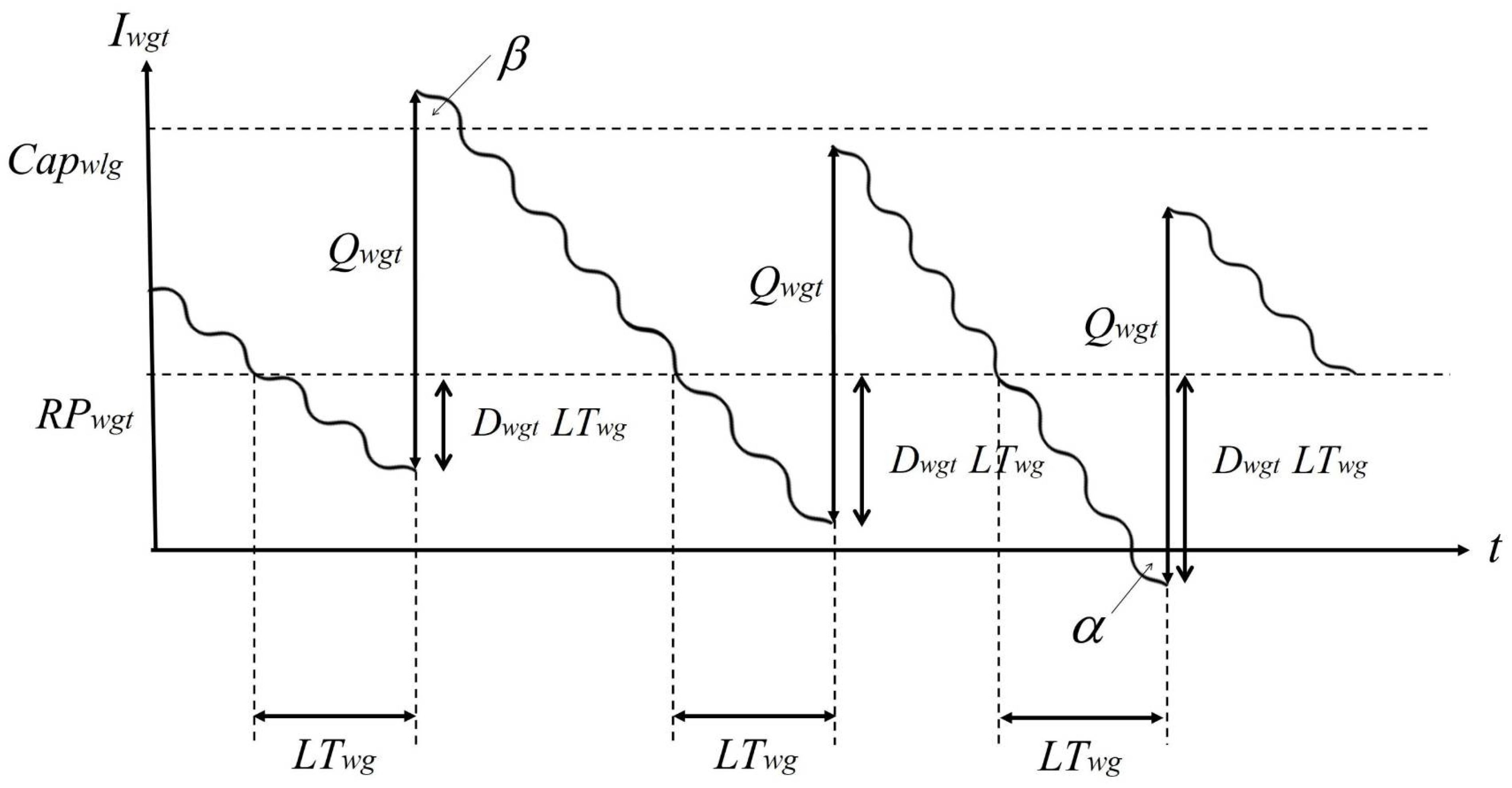
3.1. Problem Description

For each product and period, a single plant is assumed to serve a set of warehouses, which serve a set of hubs, which in turn serve the final customers with stochastic demands. The customer demands are normally distributed and independent. The demands are independent across different customers and over time. Warehouses cannot directly serve the final customers. Each customer is served by a single hub for each product and period. Each hub is served by a single warehouse for each product and period. The problem parameters such as customer demands vary over the planning horizon. Facility location-allocation and modular capacity selection decisions are made for warehouses and hubs for each product and period. We adopt the terms “open capacity”, “temporarily closed capacity”, and “existing capacity” of a facility in this paper, according to Jena et al. [13]. The open capacity is available for use. The temporarily closed capacity is temporarily not available for use and can be reopened later. The existing capacity is the combination of the open and temporarily closed capacity. Over the planning horizon, the permanent closing of capacity is not allowed in the proposed model. That is, for each product, a located facility has an open capacity level lp and an existing capacity level np (denoted by capacity levels (lp, np)) in period t−1, and capacity levels (l, n) in period t. The following constraints are imposed: $0\le lp\le np$, $0\le l\le n$, and $1\le np\le n$ (i.e., the existing capacity of a facility in period t cannot be lower than that in period t − 1). Five facility location and modular capacity adjustment costs are considered: (i) construction cost, (ii) operating fixed cost, (iii) non-operating fixed cost, (iv) reopen cost, and (v) temporary close cost.

Inventory control decisions are made at the warehouses for each product and period. There are no inventory control decisions for hubs, as these are deployed for freight transfer and consolidation. The continuous-review policy is assumed at warehouses. The capacity restrictions of vehicles in transportation from plants to warehouses can be adopted as maximum order quantity constraints at warehouses [15]. The user-specified lower limit of the implied maximum order quantity and the user-specified upper limit of reorder points from Punyim et al. [16] are employed. The level of service associated with the unfulfilled demands during the lead time for warehouses and the level of service associated with the capacity violation at the peak demands for warehouses and hubs are considered. The overall open capacity constraints for combined products at warehouses and hubs for each period are modeled.

3.2. Notations

The notations for deterministic parameters and decision variables are given.

3.2.1. Deterministic Parameters

• F¹ = Set of candidate warehouses.
• F² = Set of candidate hubs.
• F = Set of candidate facilities F¹∪ F².
• CL = Set of modular capacity levels = {0, 1, …, NCL}.
• G = Set of products.
• C = Set of customers.
• T = Set of time periods.
• N_t = Number of days in period t.
• W = Weight of total number of different located facilities over the planning horizon.
• α = Probability of unfulfilled demand during the lead time at warehouses.
• β = Maximum probability of inventory capacity violation at warehouses.
• γ = Maximum probability of violation of daily throughput capacity at hubs.
• z_1−α= The lower 100(1 − α) percentage points of standard normal distribution.
• d_ij = Roadway distance between nodes i and j.
• rUL = A fraction of inventory capacity as a practical upper limit of reorder point at warehouses.
• rLL = A fraction of maximum order quantity as a lower limit of the implied maximum order quantity.

For each facility i and period t:

• AllCap_i,t = Overall open capacity for combined products at facility i ∈ F in period t.

For each product g:

• l_ig and n_ig = Initial open capacity level and initial existing capacity level at facility i.
• RC_wg = Unit transportation cost between plant and warehouse w (USD/product unit/day).
• TC_ig = Unit transportation cost for vehicles based at facility i ∈ F (USD/distance unit/product unit).
• OC_wg = Fixed ordering cost at warehouse w (USD/order).
• HC_wg = Unit holding cost at warehouse w (USD/product unit/day).
• LT_wg = Lead time that the plant takes to fulfill an order from warehouse w (day).

For each customer c, product g, and period t:

• μ_cgt and σ²_cgt = Mean and variance of stochastic daily demand of customer c (independent and normally distributed across products, customers, and periods) (product unit/day and (product unit/day)²).

For each facility i, modular capacity level l, and product g:

• Cap_ilg = Facility capacity (inventory capacity for warehouse and daily throughput capacity for hub) for l open capacity levels (product unit).
• Q_wlg^max = Maximum order quantity which can be set as the vehicle capacity from the plant to warehouse w with l open capacity levels (product unit).
• CON_ilg = Cost for constructing l capacity levels (USD).
• OF_ilg = Operating fixed cost with l open capacity levels during a period (USD).
• NF_ilg = Non-operating fixed cost to maintain l temporarily closed capacity levels during a period (USD).
• Reopen_ilg = Cost to reopen l capacity levels (USD).
• Close_ilg = Cost to temporarily close l capacity levels (USD).

For each facility I, product g, and period t:

• f_lp,l,np,n^igt = Capacity adjustment cost (USD) to change from open and existing capacity levels (lp, np) in period t − 1 to (l, n) in period t, calculated from Equation (1) [13]:

f_lp,l,np,n^igt = CON_i,ncon,g + OF_i,nof,g + NF_i,nnf,g + Reopen_i,nreo,g + Close_i,nclo,g

(1)

where:

• ncon = n − np Capacity levels to be constructed in period t.
• nof = l Open capacity levels to be operated in period t.
• nnf = n − l Temporarily closed capacity levels to be maintained in period t.
• nreo = max{0, (l − lp)-(n − np)} Capacity levels to be reopened in period t.
• nclo = max{0, (lp − l) + n − np} Capacity levels to be closed temporarily in period t.

For example, for located facility i serving product g with open and existing capacity levels (0,2) in period t − 1 and the capacity levels (1,4) in period t, the associated capacity adjustment cost is f_0,2,1,4^igt with ncon= 2, nreo = 0, and nclo = 1.

Table 2. Capacity adjustment cost for facility i serving product g in period t.

Period t − 1	Period t	ncon	nof	nnf	nreo	nclo
Open and Existing Modular Capacity Levels (lp, np)	Open and Existing Modular Capacity Levels (l, n)	=n − np	=l	=n − l	= max{0, (l − lp) − (n − np)}	max{0, (lp − l) + n − np}
(0, 2)	(1, 2)	0	1	1	1	0
(0, 2)	(1, 3)	1	1	2	0	0
(0, 2)	(1, 4)	2	1	3	0	1

illustrates additional examples of ncon, nreo, and nclo for determining the capacity adjustment cost.

3.2.2. Decision Variables

The decision variables are described as follows.

• yy_i = 1 If facility i ∈ F is established over the planning horizon; and 0 otherwise.
• $y_{lp,l,np,n}^{i,g,t}$ = 1 If facility I ∈ F changes its capacity levels (lp, np) in period t − 1 to (l, n) in period t for product g; and 0 otherwise ∀lp ≤ np, l ≤ n, np ≤ n.
• $x_{(w,l,n),(h,\widehat{l},\widehat{n})}^{cgt}$ = 1 If product-g period-t demand of customer c is served by hub h with capacity levels ($\widehat{l},\widehat{n}$), which is served by warehouse w with capacity levels (l, n); and 0 otherwise.
• RP_wgt; SS_wgt; Q_wgt = Reorder point; safety stock; order quantity for product g at warehouse w in period t (product unit).
• ED_igt and VD_igt = Mean and variance of D_igt, daily product-g demand served by facility i ∈ F in period t (product unit/day and (product unit/day)²).
• AllCap_i,t = Overall open capacity of combined products at facility i ∈ F in period t (product unit).

3.3. Mathematical Model

We propose a mixed-integer non-linear formulation. Objective (2) minimizes z, the weighted summation of the number of different located facility locations over the planning horizon and the total estimated cost (EC). EC is composed of the first-echelon cost in (3) and the second-echelon cost in (4). The first term in (3) is the warehouse capacity adjustment cost; the second term is the ordering and holding costs for continuous-review policies at warehouses; and the third term is the direct transportation costs from plants to warehouses and between warehouses and hubs. The first term in (4) is the hub capacity adjustment cost, and the second term is the direct transport cost between hubs and customers.

$$\min z={\displaystyle \sum _{v=1}^2{z}^v}={\displaystyle \sum _{v=1}^2(W{\displaystyle \sum _{i\in F^v}y{y}_i}+{\displaystyle \sum _{t\in T}{\displaystyle \sum _{g\in G}E{C}_{gt}^v}})}$$

(2)

$$\begin{gathered} E{C}_{gt}^1={\displaystyle \sum _{i\in F^1}^{}{\displaystyle \sum _{np\in CL}^{}{\displaystyle \sum _{n=n1}^{NCL}{\displaystyle \sum _{lp=0}^{np}{\displaystyle \sum _{l=0}^n{f}_{lp,l,np,n}^{i,g,t}·y_{lp,l,np,n}^{i,g,t}}}}}} \\ +N_t{\displaystyle \sum _{w\in F^1}^{}(\frac{O{C}_{wg}}{Q_{wgt}}·E{D}_{wgt}+H{C}_{wg}(\frac{Q_{wgt}}{2}+z_{1-\alpha }L{T}_{wg}\sqrt{V{D}_{wgt}})} \\ +N_t{\displaystyle \sum _{w\in F^1}^{}{\displaystyle \sum _{n=1}^{NCL}{\displaystyle \sum _{l=1}^n{\displaystyle \sum _{h\in F^2}^{}{\displaystyle \sum _{\widehat{n}=1}^{NCL}{\displaystyle \sum _{\widehat{l}=1}^{\widehat{n}}{\displaystyle \sum _{c\in C}^{}\left(R{C}_{wg}+T{C}_{hg}·2d_{hc}\right)·{\mu }_{cgt}·x_{(w,l,n),(h,\widehat{l},\widehat{n})}^{cgt}}}}}}}} \end{gathered}$$

(3)

$$E{C}_{gt}^2={\displaystyle \sum _{i\in F^2}^{}{\displaystyle \sum _{np\in CL}^{}{\displaystyle \sum _{n=n1}^{NCL}{\displaystyle \sum _{lp=0}^{np}{\displaystyle \sum _{l=0}^n{f}_{lp,l,np,n}^{i,g,t}·y_{lp,l,np,n}^{i,g,t}}}}}}+N_t{\displaystyle \sum _{w\in F^1}^{}{\displaystyle \sum _{n=1}^{NCL}{\displaystyle \sum _{l=1}^n{\displaystyle \sum _{h\in F^2}^{}{\displaystyle \sum _{\widehat{n}=1}^{NCL}{\displaystyle \sum _{\widehat{l}=1}^{\widehat{n}}{\displaystyle \sum _{c\in C}^{}\left(T{C}_{wg}·2d_{wh}\right)·{\mu }_{cgt}·x_{(w,l,n),(h,\widehat{l},\widehat{n})}^{cgt}}}}}}}}$$

(4)

Constraint (5) guarantees the product demand of each customer in each period is served by a hub, which is served by a warehouse. Different hubs can serve a customer, and different warehouses can serve a hub for different products. Constraint (6) relates capacity adjustment variables in periods t − 2 and t − 1 (i.e., $y_{lp,l,np,n}^{i,g,t-1}$) to those in periods t − 1 and t (i.e., $y_{l,lp,n,np}^{i,g,t}$) at warehouses and hubs. From Constraint (6), for product g, period t − 1, and facility i with its open and existing capacity levels l and n, the existing capacity level of facility i in period t cannot be lower than that in period t − 1, and the existing capacity of facility i in period t − 1 cannot be lower than that in period t − 2. That is, a modular capacity level cannot be permanently closed. Constraint (6) also enforces that for each period t and product g, facility i can have its open capacity level l ranging from 0 to its existing capacity level n. Then, the number of temporarily closed capacity levels at facility i for product g and period t is n-l. Constraint (7) initializes the open and existing capacity levels in period 0. Note that the initial (i.e., period 0) open and existing capacity levels for facility i and product g are l_ig and n_ig. For each product, period, and facility, Constraint (8) ensures that at most one capacity adjustment variable is selected. Constraints (9) and (10) are the relationships between demand allocation variables and facility capacity adjustment variables in each period.

$${\displaystyle \sum _{w\in F^1}^{}{\displaystyle \sum _{n=1}^{NCL}{\displaystyle \sum _{l=1}^n{\displaystyle \sum _{h\in F^2}^{}{\displaystyle \sum _{\widehat{n}=1}^{NCL}{\displaystyle \sum _{\widehat{l}=1}^{\widehat{n}}{x}_{(w,l,n),(h,\widehat{l},\widehat{n})}^{cgt}}}}}}}=1\hspace{1em}\forall c,g,t$$

(5)

$${\displaystyle \sum _{np=0}^n{\displaystyle \sum _{lp=0}^{np}{y}_{lp,l,np,n}^{i,g,t-1}}}={\displaystyle \sum _{np=n}^{NCL}{\displaystyle \sum _{lp=0}^{np}{y}_{l,lp,n,np}^{i,g,t}}}\hspace{1em}\forall i\in F;n\in CL;l=0,\dots ,n;g\in G;t=2,\dots ,\left|T\right|$$

(6)

$${\displaystyle \sum _{n=0}^{NCL}{\displaystyle \sum _{l=0}^n{y}_{l_{ig},l,n_{ig},n}^{i,g,1}}}=1\hspace{1em}\hspace{1em}\forall i\in F,g\in G$$

(7)

$${\displaystyle \sum _{np=0}^{NCL}{\displaystyle \sum _{n=np}^{NCL}{\displaystyle \sum _{lp=0}^{np}{\displaystyle \sum _{l=0}^n{y}_{lp,l,np,n}^{igt}}}}}\le 1\hspace{1em}\forall i\in F,g,t$$

(8)

$$x_{(w,l,n),(h,\widehat{l},\widehat{n})}^{cgt}\le {\displaystyle \sum _{np=0}^{NCL}{\displaystyle \sum _{lp=0}^{np}{y}_{lp,l,np,n_{}}^{w,g,t}}} \mathrm{and} x_{(w,l,n),(h,\widehat{l},\widehat{n})}^{cgt}\le {\displaystyle \sum _{np=0}^{NCL}{\displaystyle \sum _{lp=0}^{np}{y}_{lp,\widehat{l},np,{\widehat{n}}_{}}^{h,g,t}}}$$

$$\forall w\in F^1;h\in F^2;c\in C;g\in G;t\in T;n\in CL;\widehat{n}\in CL;l=0,\dots ,n;\widehat{l}=0,\dots ,\widehat{n}$$

(9)

$$y_{lp,l,np,n}^{w,g,t}\le {\displaystyle \sum _{c\in C}^{}{\displaystyle \sum _{h\in F^2}^{}{\displaystyle \sum _{\widehat{n}=0}^{NCL}{\displaystyle \sum _{\widehat{l}=0}^{\widehat{n}}{x}_{(w,l,n),(h,\widehat{l},\widehat{n})}^{cgt}}}}} \mathrm{and} y_{lp,l,np,n}^{h,g,t}\le {\displaystyle \sum _{c\in C}^{}{\displaystyle \sum _{w\in F^1}^{}{\displaystyle \sum _{\widehat{n}=0}^{NCL}{\displaystyle \sum _{\widehat{l}=0}^{\widehat{n}}{x}_{(w,\widehat{l},\widehat{n}),(h,l,n)}^{cgt}}}}}\forall w,h,g,t,lp,np,l,n$$

(10)

For each product and period, Constraints (11) and (12) are stochastic capacity chance constraints at warehouses and hubs, respectively. Constraint (11) is based on Miranda and Garrido [15]. Figure 2 illustrates the continuous-review inventory control policy for commodity g at warehouse w with l open capacity levels in period t. When the inventory level I_wgt falls below the reorder point RP_wgt, an order quantity Q_wgt is triggered, which will be received after the lead time LT_wg. When an order is submitted to the warehouse, the inventory level should cover the stochastic demand during the lead time (D_wgt LT_wg) with probability 1 − α: Prob(D_wgt LT_wg ≤ RP_wgt) = 1 − α. Standardizing D_wgt LT_wg in this inequality yields Constraint (18), which determines reorder points and safety stocks. The stochastic inventory capacity chance constraints ensure that the peak inventory level (RP_wgt − D_wgt LT_wg + Q_wgt) at the order arrival is within the inventory capacity Cap_wlg at the warehouse with probability 1 − β: Prob(RP_wgt − D_wgt LT_wg + Q_wgt ≤ Cap_wlg) ≥ 1 − β. Substituting (18) and standardizing D_wgt LT_wgt in this inequality yields Constraint (11). We propose Constraint (12), which is the chance constraint ensuring that the served daily demand is within the daily throughput capacity at hubs with probability 1 − γ:

$$\mathrm{Prob}(D_{hgt}\le {\displaystyle \sum _{np=0}^{NCL}{\displaystyle \sum _{n=np}^{NCL}{\displaystyle \sum _{lp=0}^{np}{\displaystyle \sum _{l=0}^{n}Ca{p}_{h,l,g}^{}·y_{lp,l,np,n}^{h,g,t})}}}}\ge 1-\gamma . \mathrm{Standardizing} D_{hgt} \mathrm{in} \mathrm{this} \mathrm{inequality} \mathrm{yields}:$$

$$\mathrm{Prob}(Z\le \frac{{\displaystyle \sum _{np=0}^{NCL}{\displaystyle \sum _{n=np}^{NCL}{\displaystyle \sum _{lp=0}^{np}{\displaystyle \sum _{l=0}^{n}Ca{p}_{h,l,g}^{}·y_{lp,l,np,n}^{h,g,t}-E{D}_{hgt}}}}}}{\sqrt{V{D}_{hgt}}})\ge 1-\gamma .$$

$$\mathrm{That} \mathrm{is}, \frac{{\displaystyle \sum _{np=0}^{NCL}{\displaystyle \sum _{n=np}^{NCL}{\displaystyle \sum _{lp=0}^{np}{\displaystyle \sum _{l=0}^{n}Ca{p}_{h,l,g}^{}·y_{lp,l,np,n}^{h,g,t}-E{D}_{hgt}}}}}}{\sqrt{V{D}_{hgt}}}\ge z_{1-\gamma }, \mathrm{and} \mathrm{this} \mathrm{leads} \mathrm{to} \mathrm{Constraint} (12).$$

For each product, period, and facility, Constraints (13) and (14) determine the means and variances, respectively, of served daily demands. Constraint (15) is the maximum order quantity constraint at warehouses. In Constraint (16), the left-hand side is the implied maximum order quantities from Constraint (11). From the computational experience in the single-echelon single-period single-product location–inventory problem by Punyim et al. [16], the implied max order quantity can be a small and impractical value, so the user-specified lower limits of the implied max order quantities are proposed. Constraint (17) enforces reorder point upper limits at warehouses. Constraint (19) enforces the overall open facility capacity for combined products. Constraints (20) and (21) are bound constraints. Constraint (22) together with Objective (2) determines yy_i.

$$Q_{wgt}+(z_{1-\alpha }+z_{1-\beta })L{T}_{wg}\sqrt{V{D}_{wgt}}\le {\displaystyle \sum _{np=0}^{NCL}{\displaystyle \sum _{n=np}^{NCL}{\displaystyle \sum _{lp=0}^{np}{\displaystyle \sum _{l=0}^{n}Ca{p}_{w,l,g}^{}·y_{lp,l,np,n}^{w,g,t}}}}}\hspace{1em}\forall w,g,t$$

(11)

$$E{D}_{hgt}+z_{1-\gamma }\sqrt{V{D}_{hgt}}\le {\displaystyle \sum _{np=0}^{NCL}{\displaystyle \sum _{n=np}^{NCL}{\displaystyle \sum _{lp=0}^{np}{\displaystyle \sum _{l=0}^{n}Ca{p}_{h,l,g}^{}·y_{lp,l,np,n}^{h,g,t}}}}}\hspace{1em}\forall h,g,t$$

(12)

$${\displaystyle \sum _{n=1}^{NCL}{\displaystyle \sum _{l=1}^n{\displaystyle \sum _{h\in F^2}^{}{\displaystyle \sum _{\widehat{n}=1}^{NCL}{\displaystyle \sum _{\widehat{l}=1}^{\widehat{n}}{\displaystyle \sum _{c\in C}^{}{\mu }_{cgt}{x}_{(w,l,n),(h,\widehat{l},\widehat{n})}^{cgt}}}}}}}=E{D}_{wgt} \mathrm{and} {\displaystyle \sum _{w\in F^1}^{}{\displaystyle \sum _{n=1}^{NCL}{\displaystyle \sum _{l=1}^n{\displaystyle \sum _{\widehat{n}=1}^{NCL}{\displaystyle \sum _{\widehat{l}=1}^{\widehat{n}}{\displaystyle \sum _{c\in C}^{}{\mu }_{cgt}{x}_{(w,l,n),(h,\widehat{l},\widehat{n})}^{cgt}}}}}}}=E{D}_{hgt} \forall w,h,g,t$$

(13)

$${\displaystyle \sum _{n=1}^{NCL}{\displaystyle \sum _{l=1}^n{\displaystyle \sum _{h\in F^2}^{}{\displaystyle \sum _{\widehat{n}=1}^{NCL}{\displaystyle \sum _{\widehat{l}=1}^{\widehat{n}}{\displaystyle \sum _{c\in C}^{}{\sigma }_{cgt}^2{x}_{(w,l,n),(h,\widehat{l},\widehat{n})}^{cgt}}}}}}}=V{D}_{wgt} \mathrm{and} {\displaystyle \sum _{w\in F^1}^{}{\displaystyle \sum _{n=1}^{NCL}{\displaystyle \sum _{l=1}^n{\displaystyle \sum _{\widehat{n}=1}^{NCL}{\displaystyle \sum _{\widehat{l}=1}^{\widehat{n}}{\displaystyle \sum _{c\in C}^{}{\sigma }_{cgt}^2{x}_{(w,l,n),(h,\widehat{l},\widehat{n})}^{cgt}}}}}}}=V{D}_{hgt} \forall w,h,g,t$$

(14)

$$0\le Q_{wgt}\le {\displaystyle \sum _{np=0}^{NCL}{\displaystyle \sum _{n=np}^{NCL}{\displaystyle \sum _{lp=0}^{np}{\displaystyle \sum _{l=0}^n{Q}_{w,l,g}^{\max }·y_{lp,l,np,n}^{w,g,t}}}}}\hspace{1em}\forall w,g,t$$

(15)

$${\displaystyle \sum _{np=0}^{NCL}{\displaystyle \sum _{n=np}^{NCL}{\displaystyle \sum _{lp=0}^{np}{\displaystyle \sum _{l=0}^{n}Ca{p}_{w,l,g}^{}{y}_{lp,l,np,n}^{w,g,t}}}}}-(Z_{1-\alpha }+Z_{1-\beta })L{T}_{wg}\sqrt{V{D}_{wgt}}\ge rLL{\displaystyle \sum _{np=0}^{NCL}{\displaystyle \sum _{n=np}^{NCL}{\displaystyle \sum _{lp=0}^{np}{\displaystyle \sum _{l=0}^n{Q}_{w,l,g}^{\max }{y}_{lp,l,np,n}^{w,g,t}}}}}\hspace{1em}\forall w,g,t$$

(16)

$$R{P}_{wgt}\le rUL{\displaystyle \sum _{np=0}^{NCL}{\displaystyle \sum _{n=np}^{NCL}{\displaystyle \sum _{lp=0}^{np}{\displaystyle \sum _{l=0}^{n}Ca{p}_{w,l,g}^{}{y}_{lp,l,np,n}^{w,g,t}}}}}\hspace{1em}\forall w,g,t$$

(17)

$$R{P}_{wgt}=E{D}_{wgt}·L{T}_{wg}+S{S}_{wgt} \mathrm{and} S{S}_{wgt}=z_{1-\alpha }L{T}_{wg}\sqrt{V{D}_{wgt}} \forall w,g,t$$

(18)

$$TotCa{p}_{i,t}^{}={\displaystyle \sum _{g\in G}^{}{\displaystyle \sum _{np=0}^{NCL}{\displaystyle \sum _{n=np}^{NCL}{\displaystyle \sum _{lp=0}^{np}{\displaystyle \sum _{l=0}^{n}Ca{p}_{i,l,g}^{}·y_{lp,l,np,n}^{i,g,t}}}}}}\le AllCa{p}_{i,t}^{}\hspace{1em}\forall i\in F,t$$

(19)

$$x_{(w,l,n),(h,\widehat{l},\widehat{n})}^{cgt}\in \{0,1\}\hspace{1em}\forall w,h,l,n,\widehat{l},\widehat{n},j,g,t \mathrm{and} y_{lp,l,np,n}^{i,g,t}\in \{0,1\}\hspace{1em}\forall i\in F,lp,np,l,n,g,t$$

(20)

$$E{D}_{igt}\ge 0, V{D}_{igt}\ge 0\hspace{1em}\forall i\in F^1\cup F^2,g,t \mathrm{and} y{y}_i^{}\in \{0,1\}\hspace{1em}\forall np,n,lp,l,g,t$$

(21)

$$y_{lp,l,np,n}^{i,g,t}\le y{y}_i^{}\hspace{1em}\forall i\in F,g\in G,t\in T,np\in CL,n\in CL\backslash \left\{0\right\},lp=0,\dots ,np;l=0,\dots ,n$$

(22)

Since (3), (11), (12), (16) and (18) are non-linear, the formulation is a mixed-integer non-linear program (MINLP). Note that Constraints (11), (15) and (18) are adapted from Miranda and Garrido [15]. Constraints (16) and (17) are based on Punyim et al. [16]. The costs of partially closing and reopening modular capacity levels in Constraints (3) and (4) and facility capacity adjustment Constraints (6)–(8) are based on Jena et al. [13]. Our contributions in the formulation include the extension of the single-echelon single-period single-product location–inventory formulation with the single-level objective by Miranda and Garrido [15] and Punyim et al. [16] to the two-echelon multi-period multi-product location–inventory formulation and the incorporation of dynamic facility capacity adjustment variables allowing partial facility closing and reopening based on Jena et al. [13]. We propose the coupling constraints on the overall open capacity of combined products in Constraint (19). We propose the stochastic daily throughput capacity chance constraints at hubs in Constraint (12). We also propose the first term in Objective (2) and Constraint (22) to account for the number of different facilities over the planning horizon in which the formulation by Jena et al. [13] does not capture.

4. Proposed Multi-Start Construction and Tabu Search Improvement Heuristic

Since the proposed MINLP is np-hard, we propose a multi-start construction and tabu search improvement heuristic (MS-CTSIH) to solve the problem. The proposed heuristic is composed of two stages: construction and improvement. The construction stage generates a feasible solution from the bottom up, i.e., a feasible second-echelon solution is constructed and becomes input to the construction of a feasible first-echelon solution. The construction stage relies on the order of candidate facilities stored in facility_sequence(v,g,t). For the initial multi-start iteration (i.e., multi-start iteration 0), facility_sequence(v,g,t) is in descending order of the maximum capacity, so that the larger facilities are located to serve demand nodes. For the remaining multi-start iterations, facility_sequence(v,g,t) are randomly ordered. Based on the selected improvement strategy s with nested tabu search procedure calls as shown in

Table 3. Nested tabu search procedures after performing a feasible move for improvement strategies.

Tabu Search Procedure	Improvement Strategy
	1	2
Swap_Demand_Node(v,g,t,s)	None	Insert_Demand_Node(v,g,t,s)
Replace_Facility(v,g,s)	None	Insert_Demand_Node(v,g,t,s) for t = t_enter, …, |T|Swap_Demand_Node(v,g,t,s) for t = t_enter, …, |T|
Replace_Facility(v,s)	None	Insert_Demand_Node(v,g,t,s) for g∈G, t = t_enter, …, |T|Swap_Demand_Node(v,g,t,s) for g∈G, t = t_enter, …, |T|
Add_Facility(v,g,s)	None	Insert_Demand_Node(v,g,t,s) for t = t_enter, …, |T|Swap_Demand_Node(v,g,t,s) for t = t_enter, …, |T|Replace_Facility(v,g)
Add_Facility(v,s)	None	Insert_Demand_Node(v,g,t,s) for g∈G, t = t_enter, …, |T|Swap_Demand_Node(v,g,t,s) for g∈G, t = t_enter, …, |T|Replace_Facility(v,s) for g∈G

Note: t_enter = the first period in the current solution affected by implementing a facility move.

and discussed in Section 4.2, the improvement stage iteratively searches for an improved feasible second-echelon solution, then iteratively searches for an improved feasible first-echelon solution. The improvement stage is repeated until no improved solution is found (Algorithm 1).

Algorithm 1: MS-CTSIH(strategy s)

The proposed tabu search improvement algorithms are the extensions of the algorithm by Punyim et al. [16], which is based on Nagy and Salhi [33], Tuzun and Burke [34], and Crainic et al. [2]. Our algorithmic contribution is on the extension to incorporate the two-echelon, multi-period, and multi-product aspects and allow temporary partial closing and reopening of modular capacities of warehouses and hubs.

A destroy and repair approach is proposed in the improvement stage to ensure the feasibility over the planning horizon. It destroys the affected part in the current solution after a move changing a facility location and reconstructs the current feasible solution. For example, for a hub addition move that locates an additional hub in period 2 for product g1, the affected part in the current solution includes the set of hub locations serving product g1, the associated open and existing capacity levels, and the allocated product g1 customers in period 2 onwards. The affected part also includes the set of hubs allocated to warehouses for product g1 in period 2 onwards. The proposed procedure will destroy these affected parts in the current solution and reconstruct the feasible current solution by calling the relevant construction procedure that relies on facility_sequence(v,g,t) in the current multi-start iteration.

As discussed in Section 5.2.1, since MS-CTSIH (strategy 1) and MS-CTSIH (strategy 2) appear non-dominated on our problem instances, MS-CTSIH is modified such that both strategies are incorporated to yield a best result. The initial solution obtained from the construction stage is used in the improvement stage with both strategies. The best solution found from the two strategies is reported. The modified MS-CTSIH is shown below (Algorithm 2).

Algorithm 2: Modified MS-CTSIH

The additional notations are first defined, followed by the common procedures and descriptions of the construction stage and improvement stage.

• Additional Variables for the Current Solution
• LF_g,t^v = The set of located facilities for echelon v, product g, and period t (facilities are warehouses if v = 1 and hubs if v = 2); UF_g,t^v = F^v\LF_g,t^v.
• N_igt^allocated = The set of demand nodes serviced by facility i ∈ F for product g and period t, i.e., customers serviced by hub h in the second-echelon problem, and hubs serviced by warehouse w in the first-echelon problem.
• L_F_g^v = The set of located facilities for echelon v and product g; U_F_g^v = F^v\L_F_g^v.
• L__F^v = The set of located facilities for echelon v; U__F^v = F^v\L__F^v.
• ocl_igt and ecl_igt = Open and existing modular capacity levels for facility i ∈ F, product g, and period t.
• EnterP_ig = The earliest period that facility i ∈F is constructed to serve product g, e.g., hub h₁ is located from periods 3 to 10 to serve product g1; then EnterP_h1,g1 = 3.
• Enter_P_i = The earliest period that facility i ∈ F is constructed to serve any product.
• z = The objective value of the current solution.
• z*= The objective value of the best solution found so far.
• z′* = The objective value corresponding to the best move.
• Algorithmic Variables
• tabu_i = The last iteration number that a move of node i (demand or facility location) is prohibited.
• tenure = Number of iterations that a move is prohibited.
• freq_ig = The frequency that facility i ∈ F enters L_F_g^v (i.e., unlocated facility i becomes a located facility serving product g) in the current solution.
• freq_i = The frequency that facility i enters L__F^v in the current solution.
• Algorithmic Parameters
• max_it₂ = Maximum number of non-improvement iterations.
• div_it₂ = Number of non-improvement iterations to activate the diversification procedure in the facility replacement phase (note that div_it₂ < max_it₂).
• MS_iterations = Number of multi-start iterations.

4.1. Stage I: Construction

The construction stage constructs an initial feasible solution for echelon v by calling Construct_Solution(v). The initial second-echelon solution (v = 2) is determined first, and the located hubs become the demand nodes for warehouses in the first-echelon problem. Construct_Solution(v) iteratively builds a feasible solution for product g and period t by calling Build_Feasible_Solution(v,g,t) for each product g and period t. The open and existing capacity levels of located facilities in period t − 1 can be adjusted in period t with associated capacity adjustment costs f_lp,l,np,n^igt. The objective function z^v for echelon v is determined (see Equation (2)). The best solution found in echelon v is set to this current solution. After the initial solution is constructed, the frequency counters (freq_ig and freq_i) are initialized for tabu search in Stage II to keep track of how often each facility enters the current solution (i.e., how often facility i serving product g is removed from U_F_g^v and inserted into L_F_g^v and how often facility i is removed from U__F^v and inserted into L__F^v). Then, freq_ig and freq_i are used in the diversification procedures to diversify the current solution in the facility replacement phase (Algorithm 3).

Algorithm 3: Construct_Solution(v)

Construct_Solution(v) calls the procedure Build_Feasible_Solution(v,g,t), which in turn calls Allocate_Demand_Nodes(v,g,t) and Determine_Inventory_Policies(g,t). These are briefly described in the following sections.

4.1.1. Procedure Build_Feasible_Solution(v,g,t)

The procedure Build_Feasible_Solution(v,g,t) takes the set of located facilities in the previous period LF_g,t−1^v, their open and existing capacity levels, and facility_sequence(v,g,t) as input. The procedure sequentially selects a facility i from facility_sequence(v,g,t) where the facilities in LF_g,t−1^v are considered first and the other unlocated facilities are considered according to their orders in the sequence. The selected facility i is located by inserting i into LF_g,t^v with its greatest feasible open capacity ocl_igt with respect to Constraint (19) (i.e., constraint of overall open capacity of combined products). The existing capacity level ecl_igt is max{ocl_igt, ecl_i,g,t−1}, which implies that the existing modular capacity level cannot be permanently closed (i.e., ecl_igt ≥ ecl_i,g,t−1). The number of temporarily closed capacity levels is ecl_igt − ocl_igt, and the number of new modular capacity levels to be constructed is ecl_igt − ecl_i,g,t−₁. The feasibility of LF_g,t^v is checked by calling Allocate_Demand_Node(v,g,t). These steps are iterated until all demand nodes are served (Algorithm 4).

Algorithm 4: Build_Feasible_Solution(v,g,t)

After all demand nodes are served, if the first echelon (v = 1) is under consideration, and the inventory control policies for warehouses are determined by calling Determine_Inventory_Policies(g,t). Note that in the second-echelon solution (v = 2), there is not any inventory in consolidation hubs. At the end of Build_Feasible_Solution(v,g,t), there are three tasks. First, the remaining located facility i in period t−1, if any, is updated as a temporarily closed facility, i.e., ocl_igt = 0 and ecl_igt= ecl_i,g,t−1. Second, any redundant open capacity levels and redundant existing capacity levels in the current solution are eliminated. However, the existing capacity level of a located facility in period t cannot be lower than that in period t − 1 (see Equation (6)). Third, the estimated cost EC_gt^v is determined from Equations (3) and (4). Note that the procedure Build_Feasible_Solution(v,g,t) is employed in the construction stage and also in the improvement stage for reconstructing a feasible solution.

4.1.2. Procedure Allocate_Demand_Nodes(v,g,t)

Given LF_g,t^v, the demand nodes are sequentially allocated to these facilities with the least transportation cost while maintaining feasibility (Constraints (12)–(14), (16) and (17)) to determine N_igt^allocated ∀i ∈ LF_g,t^v. The demand nodes are allocated in descending order of the demand size. For the first echelon (v = 1), the transportation cost for warehouse w to serve hub h is (RC_wgt + TC_wgt·2·d_wh)·ED_hgt. For the second echelon (v = 2), the transportation cost for hub h to serve customer c is TC_hgt·2·d_hc·μ_cgt. After the procedure is completed, if there is any unserved demand node, the procedure returns infeasibility. To satisfy Constraints (9) and (10), if there is a located facility i that does not serve any demand node (N_igt^allocated = ∅), its open capacity is set to zero (ocl_igt = 0) (Algorithm 5).

Algorithm 5: Allocate_Demand_Node(v,g,t)

4.1.3. Procedure Determine_Inventory_Policies(g,t)

For the first echelon (v = 1), given known ED_wgt and VD_wgt, the optimal order quantity Q_wgt can be approximated by Karush–Kuhn–Tucker conditions [35] as shown in Equation (23), guaranteeing the feasibility of Constraints (11) and (15).

$$Q_{\mathit{wgt}}=\min \{(2{\mathit{OC}}_{\mathit{wg}}·{\mathit{ED}}_{\mathit{wgt}}/{\mathit{HC}}_{\mathit{wg}}{)}^{1/2}, Q_{wlg}^{\max }, {\mathit{Cap}}_{\mathit{wlg}}-(z_{1-\alpha } + z_{1-\beta })·{\mathit{LT}}_{\mathit{wg}}·({\mathit{VD}}_{\mathit{wgt}}{)}^{1/2}\}$$

(23)

The reorder points RP_wgt and safety stocks SS_wgt are determined from Constraint (18) (Algorithm 6).

Algorithm 6: Determine_Inventory_Policies(g,t)

4.2. Stage II: Improvement

The improvement stage improves the current solution for echelon v based on the improvement strategy s by calling Improve_Solution(v,s). Improvement strategy 2 involves different nested tabu search procedure calls after performing a feasible move as shown in Table 3, whereas improvement strategy 1 does not call any nested tabu search procedure. The improvement stage calls Improve_Solution(echelon 2, s) to improve the second-echelon solution, which becomes input to Improve_Solution(echelon 1, s) to improve the first-echelon solution. The procedure Improve_Solution(v,s) improves the echelon-v solution by iteratively calling six tabu search procedures based on improvement strategy s: Insert_Demand_Node(v,g,t,s), Swap_Demand_Node(v,g,t,s), Replace_Facility(v,g,s), Replace_Facility(v,s), Add_Facility(v,g,s), and Add_Facility(v,s) (Algorithm 7).

Algorithm 7: Improve_Solution(v,s)

4.2.1. Procedures Insert_Demand_Node(v,g,t,s) and Swap_Demand_Node(v,g,t,s)

Insert_Demand_Node(v,g,t,s) tries re-allocating a demand node of product g in period t currently served by a located facility to be served by another. Swap_Demand_Node(v,g,t,s) tries swapping two demand nodes of product g in period t that are currently served by two distinct located facilities. From Table 3, for both strategies, there is no nested procedure call after implementing a feasible move in Insert_Demand_Node(v,g,t,s). After implementing a demand node swap move in Swap_Demand_Node(v,g,t,s), according to improvement strategy 2, the nested procedure Insert_Demand_Node(v,g,t,s) is called in order to thoroughly search the feasible region. The procedures Insert_Demand_Node(v,g,t,s) and Swap_Demand_Node(v,g,t,s) have common steps, as shown below (Algorithm 8).

Algorithm 8: Insert_Demand_Node(v,g,t,s)/Procedure Swap_Demand_Node(v,g,t,s)

The sub-procedures to find the best feasible demand node move in Insert_Demand_Node(v,g,t,s) and Swap_Demand_Node(v,g,t,s) are find_best_demand_node_insertion_move(v,g,t) and find_best_demand_node_swap_move(v,g,t), which are described in the next sub-sections.

Sub-Procedure find_best_demand_node_insertion_move(v,g,t)

The sub-procedure iteratively determines the best feasible insertion move, which is to remove demand node j* from N_i*,g,t^allocated and insert j* into N_i’*,g,t^allocated with the feasibility of Constraints (16) and (17) for echelon v = 1 and the feasibility of Constraints (12), (16) and (17) for v = 2. The other constraints are not affected by this move (Algorithm 9).

Algorithm 9: Sub-procedure find_best_demand_node_insertion_move(v,g,t)

Sub-Procedure find_best_demand_node_swap_move(v,g,t)

The sub-procedure iteratively determines the best feasible swap move, which removes j* from N_i*,g,t^allocated and j’* from N_i’*,g,t^allocated, and inserts j* into N_i’*,g,t^allocated and j’* into N_i*,g,t^allocated while maintaining the feasibility of Constraints (16) and (17) for v = 1 and the feasibility of Constraints (12), (16) and (17) for v = 2. The other constraints are not impacted by this move (Algorithm 10).

Algorithm 10: Sub-procedure find_best_demand_node_swap_move(v,g,t)

4.2.2. Procedures Replace_Facility(v,g,s) and Add_Facility(v,g,s)

Replace_Facility(v,g,s) tries replacing each currently located facility i ∈ L_F_g^v entering in period t_enter = EnterP_ig and serving product g by each unlocated facility i’ ∈ U_F_g^v. The affected parts of the current solution from period t_enter to |T| for product g are destroyed and repaired by calling Build_Feasible_Solution(v,g,t) such that i ∈ UF_gt^v, j ∈ LF_gt^v, and EnterP_i’,g = t_enter. The procedure Replace_Faciltiy(v,g,s) calls the nested tabu search procedures according to improvement strategy s (see Table 3) after implementing a feasible move. Furthermore, the diversification procedure is employed in Replace_Facility(v,g,s) to escape from the local optimum by diversifying the current solution. If the diversification activation criterion (i.e., it_{2 =} div_it2) is satisfied, the diversification procedure tries replacing half of the located facilities i∈ L_F_g^v with greater freq_ig with unlocated facilities j ∈ U_F_g^v with lower freq_jg. The affected parts in the current solution are destroyed from the first affected period to |T| and repaired by calling Build_Feasible_Solution(v,g,t).

Add_Facility(v,g,s) tries adding each unlocated facility i ∈ U_F_g^v to serve product g by entering it at each existing entering period t_enter ∈{EnterP_jg ∀j ∈ L_F_g^v}. The destroy and repair approach similar to that in Replace_Facility(v,g,s) is employed. The procedure Add_Faciltiy(v,g,s) calls the nested tabu search procedures according to the improvement strategy s as shown in Table 3. Replace_Faciltiy(v,g,s) and Add_Facility(v,g,s) share common steps, as shown below (Algorithm 11).

Algorithm 11: Replace_Facility(v,g,s)/Procedure Add_Facility(v,g,s)

The sub-procedures to find the best feasible facility move in Replace_Facility(v,g,s) and Add_Facility(v,g,s) are find_best_facility_replacement_move(v,g) and find_best_facility_addition_move(v,g), which are described in the next sub-sections.

Sub-Procedure find_best_facility_replacement_move(v,g)

The sub-procedure iteratively determines the best feasible facility replacement move for product g and echelon v. A facility replacement move removes I from L_F_g^v with its entering period t_enter = EnterP_ig, removes i’ from U_F_g^v, destroys the current solution from period t_enter to |T|, and repairs the current solution by calling Build_Feasible_Solution(v,g,t) such that i ∈ UF_gt^v, i’ ∈ LF_gt^v, and EnterP_i’,g = t_enter. The destroy and repair approach is employed because simply replacing i by i’ greatly impacts the feasibility of the current solution from period t_enter to |T| (Algorithm 12).

Algorithm 12: Sub-procedure find_best_facility_replacement_move(v,g)

Sub-Procedure find_best_facility_addition_move(v,g)

The sub-procedure iteratively determines the best feasible addition move for product g and echelon v. For each period t_enter ∈ {EnterP_jg ∀j ∈ L_F_g^v} (i.e., each entering period of a located facility in the current solution), an addition move allows an unlocated facility I ∈ U_F_g^v to enter the current solution in period t_enter. This move destroys the current solution from period t_enter onwards and repairs the current solution by calling Build_Feasible_Solution(v,g,t) such that i ∈ LF_gt^v. The destroy and repair approach is employed because the demand allocations are required to re-allocate demands to the new set of located facilities from period t_enter onwards (Algorithm 13).

Algorithm 13: Sub-procedure find_best_facility_addition_move(v,g)

4.2.3. Procedures Replace_Facility(v,s) and Add_Facility(v,s)

Replace_Facility(v,s) tries replacing each currently located facility i ∈ L__F^v serving all products by each unlocated facility j ∈ U__F^v. Replace_Facility(v,s) is similar to Replace_Facility(v,g,s). The destroy and repair approach in Replace_Facility(v,s) considers all products over the affected periods, whereas that in Replace_Facility(v,g,s) considers only product g. The nested tabu search procedures in Replace_Facility(v,s) thoroughly search the feasible region for all products according to improvement strategy s as shown in Table 3, whereas those in Replace_Facility(v,g,s) search the feasible region only for product g. The diversification procedure employed in Replace_Facility(v,s) tries replacing half of located facilities i ∈ L__F^v with greater freq_i by unlocated facilities i’ ∈ U__F^v with lower freq_i′.

Add_Facility(v,s) tries adding each unlocated facility i ∈ U__F^v to serve any product by entering it at each existing entering period t_enter∈{Enter_P_j ∀j ∈ L__F^v}. The destroy and repair approach in Add_Facility(v) considers all products over the affected periods. The nested tabu search procedures in Add_Facility(v,s) thoroughly search the feasible region for all products according to improvement strategy s (see Table 3). Note that Replace_Facility(v,s) and Add_Facility(v,s) can perform better than Replace_Facility(v,g,s) and Add_Facility(v,g,s) when the weight of total number of different located facilities W is relatively high (Algorithm 14).

Algorithm 14: Replace_Facility(v,s)/Procedure Add_Facility(v,s)

The sub-procedures to find the best feasible facility move in Replace_Facility(v,s) and Add_Facility(v,s) are find_best_facility_replacement_move(v) and find_best_facility_addition_move(v), which are described in the next sub-sections.

Sub-Procedure find_best_facility_replacement_move(v)

The sub-procedure iteratively determines the best feasible facility replacement move for all products in echelon v. A facility replacement move removes i from L__F^v with its entering period t_enter = Enter_P_i, removes i’ from U__F^v, destroys the current solution from period t_enter to |T|, and repairs the current solution by calling Build_Feasible_Solution(v,g,t) ∀g ∈ G such that i ∈ UF_gt^v, i’ ∈ LF_gt^v and Enter_P_i’ = t_enter (Algorithm 15).

Algorithm 15: Sub-procedure find_best_facility_replacement_move(v)

Sub-Procedure find_best_facility_addition_move(v)

The sub-procedure iteratively determines the best feasible addition move for all products in echelon v. For each period t_enter∈{Enter_P_j ∀j ∈ L__F^v} (i.e., each entering period of a located facility in the current solution), an addition move allows an unlocated facility i ∈ U__F^v to enter the current solution in period t_enter. This move destroys the current solution from period t_enter onwards and repairs the current solution by calling Build_Feasible_Solution(v,g,t) ∀g ∈ G such that i ∈LF_gt^v (Algorithm 16).

Algorithm 16: Sub-procedure find_best_facility_addition_move(v)

5. Computational Experiences

The proposed heuristic is implemented in C++. The computational experiments were conducted on a desktop computer with a 1.80 GHz Intel Core i7 processor and 16 GB of RAM. First, the data are described, followed by computational results.

5.1. Data

Since there are no standard test problems for the considered problem, the large and small problem instances are developed as follows.

5.1.1. Large Problem Instance

Three product types (g1–g3), five periods (t1–t5), and three modular capacity levels (l1–l3) are considered. The mixed random and clustered configuration of customer data from Solomon [36] (nodes 1–100) is employed (x and y coordinates within the respective ranges (0, 95) and (3, 85)). The mean customer demands μ_c,g1,t1, μ_c,g2,t1, and μ_c,g3,t1 are the respective C1, R1, and RC1 demands in Solomon [36]. The coefficient of variation of 0.5 is employed to determine the demand variances. The mean demands for other periods (t2 to t5) are assumed μ_c,g,t = f(t,g) μ_c,g,t1, where f(t,g) is a multiplicative factor for the mean demand of product g in period t, as shown in

Table 4. Factor f(t, g) for the large problem instance.

Period	g1	g2	g3
1	1	1	1
2	1.1	1.2	0.9
3	1.21	1.44	0.81
4	1.331	1.296	0.972
5	1.4641	1.1664	1.1664

. There are three demand profiles for the three products. Product g1 has demand profile 1 representing an increasing trend over the horizon by the constant growth rate of 10 percent per period. Product g2 has demand profile 2 representing a fluctuating trend by the growth rates of 20, 20, −10, and −10 percent per period for periods t2, t3, t4, and t5, respectively. Product g3 has demand profile 3 representing a fluctuating trend by the growth rates of −10, −10, +20, and +20 percent per period for periods t2, t3, t4, and t5, respectively.

There are 20 candidate warehouses and 20 candidate hubs. The x and y coordinates of candidate hubs are randomly generated from the ranges (0, 95) and (3, 85), respectively. These ranges cover the urban area where customers are located. The x and y coordinates in the ranges (−12, 105) and (−12, 100), respectively, cover the study area, which is composed of the urban area in the center and the suburban area in the outer area. The x and y coordinates of candidate warehouses are randomly generated from this outer area.

Table 5. Data of candidate warehouses and hubs.

Warehouse	x	y	Capw,l1,g	OFw,l1,g	Hub	x	y	Caph,l1,g	OFh,l1,g
w1	−11	63	250	400	h1	1	7	90	200
w2	30	−4	200	200	h2	3	68	70	100
w3	13	93	250	400	h3	91	27	90	200
w4	49	90	250	400	h4	66	36	90	200
w5	102	23	200	200	h5	42	82	70	100
w6	47	−4	300	600	h6	12	58	110	300
w7	31	92	250	400	h7	74	51	90	200
w8	−6	10	200	200	h8	31	18	70	100
w9	100	65	250	400	h9	33	83	90	200
w10	66	−12	200	200	h10	19	63	70	100
w11	−3	26	300	600	h11	18	31	110	300
w12	−2	77	250	400	h12	35	21	90	200
w13	99	71	200	200	h13	29	63	70	100
w14	7	−10	250	400	h14	58	71	90	200
w15	87	88	250	400	h15	89	47	90	200
w16	99	47	250	400	h16	1	48	90	200
w17	70	97	200	200	h17	59	56	70	100
w18	−8	38	200	200	h18	19	69	70	100
w19	90	−6	200	200	h19	65	16	70	100
w20	105	11	250	400	h20	30	30	90	200

shows the x and y coordinates for candidate facilities. Table 5 also shows the values of a single modular capacity (Cap_w,l1,g and Cap_h,l1,g) and associated operating fixed costs (OF_w,l1,g and OF_h,l1,g) for all products. The facility capacities and operating fixed costs for two and three modular capacity levels are two and three times as much, respectively, as those for one capacity level, e.g., Cap_w,l2,g = 2*Cap_w,l1,g. For warehouses, the maximum order quantity $Q_{wlg}^{\max }$ is assumed 0.25Cap_wlg.

For all warehouses and products, the unit transport costs from plants to warehouses RC_wg are USD 1/product unit/day, unit transport costs from warehouses to hubs TC_wg are USD 0.05/distance unit/product unit, unit ordering costs OC_wg are USD 50/order, unit holding costs HC_wg are USD 1/product unit/day, and lead times LT_wg are 1 day. For all hubs and products, the unit transport costs from hubs to customers TC_hg are USD 0.075/distance unit/product unit. For all facilities and periods, the overall capacities (AllCap_wt and AllCap_ht) are 10,000 product units. For all facilities, capacity levels, and products, the construction costs (CON_ilg), non-operating fixed cost (NF_ilg), temporary close costs (Close_ilg), and reopen costs (Reopen_ilg) are assumed to be generated by multiplying OF_ilg with 10, 0.2, 0.25, and 0.5, respectively. There is not any located facility at period 0 for all products, i.e., l_ig = n_ig = 0 ∀i ∈ F, g ∈ G.

The service level for stockout during lead time (1 − α), that for inventory capacity violation at warehouses (1 − β), and that for the daily throughput capacity violation at hubs (1 − γ) is 97.5%. The other problem parameters are rUL = 0.9 and rLL = 0.5. The employed algorithmic parameters are max_it₂ = 5 and div_it₂ = 4.

5.1.2. Small Problem Instance

The small problem instance is created based on the large problem instance. The first two products (g1, g2), the first three periods (t1, t2, t3), two modular capacity levels (l1, l2), the first three candidate warehouses (w1, w2, w3), the first three candidate hubs (h1, h2, h3), and the first nine customers (customers one to nine) of the large problem instance are considered. There are two demand profiles for the two products, as shown in

Table 6. Factor f(t, g) for the small problem instance.

Period	g1	g2
1	1	1
2	0.75	1.5
3	1	2

. Product g1 has a fluctuated demand profile by the growth rates of −25 and +33.33 percent per period for periods t2 and t3, respectively. Product g2 has an increasing demand profile by the growth rates of 50 and 33.33 percent per period for periods t2 and t3, respectively. The other data for the small instance are the same as those for the large problem instance.

5.2. Experimental Results

The comparison of the two improvement strategies on the large instance is presented in order to determine the best strategy. The solution from the proposed heuristic and the analytical solution from a commercial solver on the small problem instance are then compared. The best solution found on the small instance is examined. Lastly, the sensitivity analyses are performed on the large problem instance.

5.2.1. Comparison of Improvement Strategies

The proposed MS-CTSIH with two improvement strategies are performed on the problem instances when using MS_iterations = 100 and varying W, the weight of total number of located facilities.

Table 7. Best objective values, iteration that found best solution, and number of located facilities (MS_iterations = 100).

(a) Large Problem Instance
W	MS-CTSIH (Strategy 1)				MS-CTSIH (Strategy 2)				Modified MS-CTSIH
	Best Obj. (×108)	Iter.	No. of Fac.	Total CPU (h)	Best Obj. (×108)	Iter.	No. of Fac.	Total CPU (h)	Best Obj. (×108)	Iter.	No. of Fac.	Total CPU (h)
107	2.91525	0	18	1.12	2.95075	0	18	1.64	2.91418	0	18	2.94
106	1.25349	31	24	0.99	1.25802	31	24	0.87	1.24970	31	23	2.15
105	1.03294	77	27	1.06	1.03815	82	28	1.47	1.03294	77	27	2.06
0	1.00320	77	28	1.10	1.01086	77	29	1.51	1.00320	77	28	3.02
(b) Small Problem Instance
W	MS-CTSIH (Strategy 1)				MS-CTSIH (Strategy 2)				Modified MS-CTSIH
	Best Obj. (×106)	Iter.	No. of Fac.	Total CPU (min)	Best Obj. (×106)	Iter.	No. of Fac.	Total CPU (min)	Best Obj. (×106)	Iter.	No. of Fac.	Total CPU (min)
107	38.4486	15	3	0.121	38.4284	15	3	0.324	38.4284	15	3	0.527
106	11.0912	0	4	0.139	11.0876	0	4	0.255	11.0876	0	4	0.463
105	7.49123	0	4	0.113	7.48756	0	4	0.250	7.48756	0	4	0.449
0	7.09123	0	4	0.113	7.08756	0	4	0.253	7.08756	0	4	0.440

shows the best objective values, multi-start iteration numbers that found the best solution, the associated number of located facilities, and total CPU time. Interestingly, MS-CTSIH (strategy 1) (no nested tabu search procedure calls) outperforms MS-CTSIH (strategy 2) on the large instance at different values of W, whereas MS-CTSIH (strategy 2) outperforms MS-CTSIH (strategy 1) on the small instance at various W values. The modified MS-CTSIH that incorporates both improvement strategies yields the best results with longer CPU time on the two problem instances at different W values. Figure 3 shows the convergence characteristics of MS-CTSIH (strategy 1), MS-CTSIH (strategy 2), and modified MS-CTSIH on the large problem instance for W = 0. MS-CTSIH (strategy 2) is slower to converge than MS-CTSIH (strategy 1), as expected, and the modified MS-CTSIH spends the longest time.

The multi-start iterations can yield an improved solution on the large instance when W is up to 10⁶, implying that facility_sequence(v,g,t) in multi-start iteration 0 (i.e., in the descending order of the maximum capacity) cannot yield the best solution. At W = 10⁷, the two strategies cannot find an improved solution over the 100 multi-start iterations. This means that facility_sequence(v,g,t) in multi-start iteration 0 can yield the least number of facilities on the large instance. However, this is not always the case, as Table 7b shows that the multi-start iterations cannot yield an improved solution on the small instance when W is up to 10⁶ but can yield an improved solution when W = 10⁷. From Table 7, as W decreases from 10⁷ to 0, the number of facilities is non-decreasing on the small instance and increases on the large instance, as expected.

5.2.2. Comparison of Proposed Heuristic and Analytical Solution Method

The proposed MINLP model is implemented in the General Algebraic Modeling System Integrated Development Environment (GAMS IDE) Release 27.2.0, and solved by GAMS/BARON, a commercial solver, which solves the problem with the branch-and-reduce algorithm. The modified heuristic with MS_iterations = 100 and the GAMS/BARON solver is performed on the small instance with W = 10⁷.

The GAMS/BARON solver, which employs the feasible solution from the construction stage as an initial solution, takes 25.02 h to find a solution with the objective value of 4.16451 × 10⁷ and the relative optimality gap of 13.10% (the lower bound of 3.62069 × 10⁷). The modified heuristic takes 0.527 min to find a solution with the objective value of 3.84284 × 10⁷ and the relative optimality gap of 5.78%. The modified algorithm yields the solution with the better relative optimality gap and much faster than GAMS/BARON. This shows the efficiency and effectiveness of the proposed heuristic on a small instance.

5.2.3. Examination of Heuristic Solution on the Small Problem Instance

The best solution found by the modified MS-CTSIH on the small instance with W = 10⁷ is examined to illustrate the feasibility and characteristics of the best solution found. From

Table 8. Best solution founded on the small problem instance (W = 10⁷).

(a) First-Echelon Solution
Period				t1					t2				t3
Product				g1			g2		g1		g2		g1		g2
located warehouse				w2			w2		w2		w2		w2		w2
open inventory capacity, Capwlg				400			200		400		400		400		400
existing inventory capacity				400			200		400		400		400		400
served mean demand, EDwgt				190			108		142.5		162		190		216
served demand variance, VDwgt				1175			431.5		660.94		970.88		1175		1726
assigned hubs				h1, h3			h1		h1, h3		h1, h3		h1, h3		h1, h3
construction cost				400,000			200,000		0		200,000		0		0
operating fixed cost				40,000			20,000		40,000		40,000		40,000		40,000
non-operated fixed cost				0			0		0		0		0		0
reopen cost				0			0		0		0		0		0
temporary close cost				0			0		0		0		0		0
transport cost (plants–warehouses), rcwgt				69,350			39,420		52,012.5		59,130		69,350		78,840
transport cost (warehouses–hubs)				310,677			122,266		181,804		236,650		310,677		381,074
holding cost, hcwgt				42,772.7			23,985.7		36,642		40,541.1		42,772.7		47,971.4
ordering cost, ocwgt				34,675			39,420		26,006.2		29,565		34,675		39,420
Continuous-Review Inventory Control Policy
order quantity, Qwgt				100			50		100		100		100		100
reorder point, RPwgt				257.19			148.71		192.89		223.07		257.19		297.43
safety stock, SSwgt				67.19			40.71		50.39		61.07		67.19		81.43
(b) Second-Echelon Solution
Period	t1				t2						t3
Product	g1		g2		g1			g2			g1			g2
located hub	h1	h3	h1		h1	h3		h1		h3	h1	h3		h1		h3
open max served daily demand, Caphlg	180	180	180		180	90		180		90	180	180		180		180
existing max served daily demand	180	180	180		180	180		180		90	180	180		180		180
served mean demand, EDhgt	120	70	108		127.5	15		123		39	120	70		116		100
served demand variance, VDhgt	850	325	431.5		604.69	56.25		814.5		156.38	850	325		1062		664
assigned customers	4, 2, 8, 9, 7	6, 3, 1, 5	1–9		2–9	1		5, 4, 9, 7, 8, 2		1, 3, 6	4, 2, 8, 9, 7	6, 3, 1, 5		5, 8, 9, 2		3, 1, 4, 6, 7
construction cost USD 1K	200	200	200		0	0		0		100	0	0		0		100
operating fixed USD 1K	20	20	20		20	10		20		10	20	20		20		20
non-operated fixed cost USD 1K	0	0	0		0	2		0		0	0	0		0		0
reopen cost (USD 1K)	0	0	0		0	0		0		0	0	5		0		0
temporary close cost (USD 1K)	0	0	0		0	2.5		0		0	0	0		0		0
transport cost (hubs– customers) (USD 1K)	431.0	341.6	415.1		479.9	72.2		452.1		189.9	431.0	341.6		407.9		486.8

, in the best solution found, the single warehouse w2 is constructed in period t1 to serve both products. Hubs h1 and h3 are constructed in period t1 to serve product g1. For product g2, only hub h1 is constructed in period t1 and hub h3 is constructed later in period t2 to accommodate the increasing demand profile for product g2.

Table 9. Total open capacities for combined products on the small problem instance.

Period	Total Mean Demand (Product Units/Day)			Total Demand Variance (Product Units/Day)2			First-Echelon Facility	Second-Echelon Facility
							w2	h1	h3
	g1	g2	all g	g1	g2	all g	all g	all g	all g
t1	190	108	298.0	1175	431.5	1606.5	600	360	180
t2	142.5	162	304.5	660.9	970.9	1631.8	800	360	180
t3	190	216	406.0	1175	1726	2901.00	800	360	360

shows that the total open capacities for combined products at facilities w2, h1, and h3 are less than the specified overall open capacity of 10,000 product units for all periods. Warehouse w2 and hub h3 have the increasing total open capacities, whereas hub h1 has the constant total open capacity. These are results of the increasing trend of total mean demands (298, 304.5, and 406 product units for periods t1, t2, and t3) and total demand variances (1606.5, 1631.8, and 2901 for periods t1, t2, and t3).

From Table 8a, two modular inventory capacity levels for product g1 are constructed at warehouse w2 in period t1 (i.e., 2 × 200 = 400 product units), and no additional modular capacity is constructed in later periods. The construction cost of USD 400,000 for two modular capacity levels for product g1 and the operating fixed cost of USD 40,000 for two capacity levels for product g1 are incurred at warehouse w2 in period t1. The numbers of open capacity levels for product g1 at warehouse w2 are constant (i.e., 2 levels = 400 product units) over the planning horizon. This is not consistent with the demand profile of product g1 that has a demand drop in period t2. This is due to Constraint (11), where the left-hand side is Q_w2,g1,t2 + (z_1−α + z_1−β)*LT_w2,g1*(VD_w2,g1,t2)^0.5 = 100 + (1.96 + 1.96)*1*(660.94)^0.5 = 200.8 product units that requires two open modular capacity levels (Cap_w2,l2,g1 = 400 product units) as opposed to one open capacity level (Cap_w2,l1,g1 = 200 product units) in order to satisfy this constraint.

A modular capacity level for product g2 is constructed at warehouse w2 in period t1, and later an additional capacity level is constructed in period t2. This is consistent with the increasing demand profile of product g2. The cost of USD 200,000 to construct a modular capacity level for product g2 is incurred at warehouse w2 in periods t1 and t2. The cost of USD 20,000 to operate a capacity level for product g2 is incurred at warehouse w2 in period t1, and the cost of USD 40,000 to operate two capacity levels for product g2 is incurred in periods t2 and t3.

The order quantities, reorder points, and safety stocks for each product at warehouse w2 can be verified from Equations (23) and (18), respectively. The holding costs, ordering costs, and transport costs from the plant to warehouses can be verified from the relevant terms in Equation (3), as shown below:

hc_wgt = N_t HC_wg (Q_wgt/2 + z_1−α LT_wg (VD_wgt)^1/2)

(24)

oc_wgt = N_t OC_wg ED_wgt/Q_wgt

(25)

rc_wgt = N_t RC_wg ED_wgt

(26)

To illustrate, for product g1 in period t1, these variables for warehouses w2 are Q_w2,g1,t1 = 100 product units, RP_w2,g1,t1 = 257.19 product units, SS_w2,g1,t1 = 67.19 product units, hc_w2,g1,t1 = USD 42,773, oc_w2,g1,t1 = USD 34,675, and rc_w2,g1,t1 = USD 69,350. These are obtained by substituting z_1−α = z_1−β = 1.96, HC_w2,g1 = 1, OC_w2,g1 = 50, RC_w2,g1 = 1, LT_w2,g1 = 1 day, Q_w2,l2,g1^max = 100, Cap_w2,l2,g1 = 400, ED_w2,g1,t1 = 190, and VD_w2,g1,t1 = 1175 into Equations (23), (18), and (24)–(26).

From Table 8b, two modular inventory capacity levels for product g1 are constructed at hubs h1 and h3 in period t1 (i.e., 2 × 90 = 180 product units at h1 and h3), and no additional modular capacity is constructed in later periods. The construction cost of USD 200,000 for two modular capacity levels for product g1 and the operating fixed cost of USD 20,000 for two capacity levels for product g1 are incurred at hubs h1 and h3 in period t1. The numbers of open capacity levels for product g1 at hub h1 are constant (i.e., two levels = 180 product units) over the planning horizon, whereas those at hub h3 are two, one, and two levels for periods t1, t2, and t3, respectively. This is consistent with the demand profile of product g1 that has a demand drop in period t2. One can examine the feasibility of constraints (12) for hub h1 serving product g1 in the three periods, where the left-hand sides (i.e., ED_h1,g1,t + z_1−γ (VD_h1,g1,t)^0.5) are 105.3, 29.7, and 105.3 product units per day that require two, one, and two open capacity levels, respectively (i.e., the right-hand sides are Cap_h1,l2,g1 = 180, Cap_h1,l1,g1 = 90, Cap_h1,l2,g1 = 180 product units, respectively). Note that hub h2 serving product g1 with Cap_h1,l1,g1 =70 can be employed to satisfy Constraint (12), but the total number of different located hubs will be increased by one and the objective will also be increased by W = 10⁷. The cost of USD 2500 to temporarily close a capacity level, the cost of USD 2000 to maintain a temporarily closed capacity level, and the cost of USD 10,000 to operate a capacity level for product g1 are incurred at hub h3 in period 2. The cost of USD 5000 to reopen a capacity level and the cost of USD 20,000 to operate two capacity levels for product g1 are incurred at hub h3 in period t3.

Two modular capacity levels for product g2 are constructed at hub h1 in period t1, and no additional capacity level is constructed at hub h1 in later periods. A modular capacity level for product g2 is constructed at hub h3 in period t2, and an additional capacity level is constructed at hub h3 in period t3. This is consistent with the increasing demand profile of product g2 with the peak demand at period t3. The cost of USD 200,000 to construct two modular capacity levels for product g2 is incurred at hub h1 in period t1, and the cost of USD 100,000 to construct an additional capacity level for product g2 is incurred at hub h3 in periods t2 and t3. The cost of USD 20,000 to operate two capacity levels for product g2 is incurred at hub h1 in all three periods. The costs of USD 10,000 and USD 20,000 to operate one level and two levels for product g2 are incurred at hub h3 in periods t2 and t3, respectively.

The customers are dynamically allocated to different hubs in different periods. For product g1, the demand is dropped in period t2, and the demands in periods t1 and t3 are the same. The customers are served by the same hubs in periods t1 and t3 (i.e., customers 4, 2, 8, 9, and 7 served by hub h1 and the others by h3), whereas in period t2 all customers are served by hub h1 and only customer 1 is served by hub h3, which has a reduced open capacity level. For product g2, all customers are served by hub h1 in period t1, and in later periods the customers are allocated to hubs h1 and h3 differently in period t2 and t3. The associated transport costs between hubs and customers are also shown in Table 8b.

5.2.4. Sensitivity Analysis

Using the modified MS-CTSIH, the sensitivity analyses of the service levels (1 − α, 1 − β, and 1 − γ), overall open inventory capacity of the combined products (AllCap_w,t), demand standard deviation, and W are performed on the large problem instance. Figure 4 shows the sensitivity analysis results. The service levels for unfulfilled demand during the lead time at warehouses (1 − α), inventory capacity violation (1 − β), and daily throughput capacity violation (1 − γ) are assumed equal. Given the other parameters being the same, three levels of 1 − α = 1 − β = 1 − γ (0.65, 0.80, and 0.95), which correspond to 65%, 80%, and 95% service levels, respectively, are considered. From Figure 4a, given all else being equal, as the service level increases from 65% to 95%, the objective function value, the number of located warehouses, and the number of located hubs also increase. The greater-objective-function solution and the greater number of located facilities are traded off with the increase in service level (i.e., more constrained problem).

Five levels of overall open inventory capacity at each warehouse w (AllCap_w,t) are considered, given all other parameters being the same. From Figure 4b, given all else being equal, the objective function value decreases (i.e., achieving a better solution) as AllCap_w,t increases (i.e., more relaxed constraints). The number of located warehouses is higher at a lesser value of AllCap_w,t, as expected. Five levels of standard deviation factor (SDF), which is a multiplicative factor for the demand variance at each customer and product, are considered. From Figure 4c, as the SDF increases, the objective function value and the number of located hubs also increase. From Figure 4d, the greater the W value the higher the objective function value. As W increases, the number of located facilities decreases, as expected.

5.2.5. Discussion

For the industry, the proposed model and heuristic can enable logistics companies to make better strategic decisions on the siting and sizing of warehouses and hubs, and to make better tactical decisions on demand node allocations and inventory control policies at warehouses in order to service uncertain customer demands for different products over the planning horizon. The logistics company can prepare the investment budget in each period to construct the planned number of modular capacity levels at certain warehouses and hubs to serve different products. They can prepare a proper plan (e.g., workforce planning) to temporarily close down a certain number of modular capacity levels at certain facilities in a certain period that is predicted to have a reduction in demand of certain products. Similarly, they can also prepare a proper plan to reopen a number of modular capacity levels at some warehouses and hubs in a period in which the demand of a product is predicted to be bounced back. Furthermore, the customer allocation (customers allocated to hubs) and the hub allocation (hubs allocated to warehouses) are different over different periods for various products in order to achieve the least cost, while maintaining the feasibility of diverse constraints such as the hub service level constraints (in terms of daily throughput capacity violation) and maximum order quantity constraints. The logistics company can control the inventories at warehouses for different products and periods by using the optimal order quantities, reorder points, and safety stocks, all of which satisfy the specified inventory service level constraints (in terms of inventory capacity violation and stockouts during lead times).

The weight on the number of located facilities can be changed from a common constant to facility-location-specific weights W_i ∀i ∈ F. The weight W_i can be set to the monetary value of the spatial and physical impacts in terms of geologic, biologic, or geographic features (e.g., land use, forest type, and habitat impacts) [37,38], or the monetary value of the environmental impacts in terms of water, air, soils, ecosystems, and aesthetics [39] when facility i is located. As such, the objective function can be modified as:

$$\min z={\displaystyle \sum _{v=1}^2{z}^v}={\displaystyle \sum _{v=1}^2({\displaystyle \sum _{i\in F^v}{W}_{i}y{y}_i}+{\displaystyle \sum _{t\in T}{\displaystyle \sum _{g\in G}E{C}_{gt}^v}})}$$

With this objective, the proposed model and heuristic can determine the best solution that explicitly accounts for the spatial, physical, and environmental impacts in addition to the economic impacts (i.e., facility, inventory, and transportation costs).

6. Conclusions

In this paper, the two-echelon multi-period multi-product location–inventory problem with partial facility closing and reopening is studied. The modular capacity levels at facilities can be temporarily and partially closed at a period and reopened in a later period. For each product and period, a single plant is assumed to serve warehouses that serve hubs, which in turn serve the final customers with independent and normally distributed demands. The overall open capacity for combined products at a facility is considered. Continuous-review inventory control decisions are made at located warehouses. There are no such decisions for located hubs, which are employed for freight transfer and consolidation. The problem parameters such as customer demands can vary over the horizon. The proposed formulation is a mixed-integer non-linear model. The multi-start construction and tabu search improvement heuristic is developed. Two improvement strategies (with and without nested tabu search procedure calls) are proposed, and the modified heuristic incorporating both strategies is developed. The comparison of two improvement strategies in the tabu search improvement stage shows that MS-CTSIH (strategy 1) and MS-CTSIH (strategy 2) are non-dominated on the small and large problem instances at different values of W, the weight of the total number of located facilities. The modified MS-CTSIH incorporating both improvement strategies yields the best results on the small and large instances. The comparison of the modified MS-CTSIH and the exact solution method on the small problem instance shows the effectiveness and efficiency of the proposed heuristic. The modified MS-CTSIH spends 0.527 min to obtain the best solution with the optimality gap of 5.78%, whereas the exact solution method spends 25.02 h to obtain the best solution with the optimality gap of 13.10%. The best solution from the small instance is thoroughly examined to illustrate the feasibility with respect to various constraints. The small instance problem is used to portray how the construction costs, operating fixed costs, temporary closing costs, non-operating fixed costs, and reopening costs are incurred at a facility serving a product in a period according to changes in modular capacity levels due to the associated demand profile. The inventory control policies at warehouses in the best solution are also examined. The sensitivity analyses of the service levels and overall open inventory capacity of the combined products, demand standard deviation, and the weight of the total number of located facilities are performed to study how the objective function value and the number of located facilities change with the change in these problem parameters.

For the industry, the proposed model and heuristic can be used as a tool for logistics companies to make better strategic decisions on the siting and sizing of warehouses and hubs, and to make better tactical decisions on demand node allocations and inventory control policies in order to service uncertain customer demands of different products over the planning horizon in the urban goods distribution. The schedule of construction, temporary partial closing, and reopening of modular capacities of warehouses and hubs to serve various products allows the logistics company to prepare an appropriate plan such as workforce management as well as the investment budget. With the continuous-review inventory control policies at warehouses, the optimal order quantities, reorder points, and safety stocks at warehouses for various products in different periods can be employed such that the prespecified inventory service level constraints (in terms of inventory capacity violation and stockouts during lead times) are satisfied. The demand node allocation differs for different products in different periods and yields the least cost while diverse constraints such as hub service level constraints (in terms of daily throughput capacity violation) are satisfied. In addition to the economic impacts (i.e., facility, inventory control, and transportation costs), the proposed model and heuristic can explicitly account for the spatial, physical, and environmental impacts from the facility siting via the facility-location-specific weight representing the monetary value of such impacts.

For future research, the proposed model and heuristic can be extended to explicitly account for the monetary value of greenhouse gas emission from warehouse operation, hub operation, and transportation. The other future research directions include the incorporation of different inventory control policies such as periodic review, the consideration of correlated customer demands, and the integration of the vehicle routing problem into the joint location–inventory problem.

References

1. Silva, A.; Aloise, D.; Coelho, L.C.; Rocha, C. Heuristics for the dynamic facility location problem with modular capacities. Eur. J. Oper. Res. 2021, 290, 435–452. [Google Scholar] [CrossRef]
2. Crainic, T.G.; Sforza, A.; Sterle, C. Tabu search heuristic for a two-echelon location-routing problem, Research Report, interuniversity research centre on enterprise networks, logistics and transportation. In CIRRELT-2011-07; CIRRELT: Montréal, QC, Canada, 2011. [Google Scholar]
3. Crainic, T.G.; Ricciardi, N.; Storchi, G. Advanced freight transportation systems for congested urban areas. Transp. Res. Part C Emerg. Technol. 2004, 12, 119–137. [Google Scholar] [CrossRef]
4. Crainic, T.G.; Ricciardi, N.; Storchi, G. Models for evaluating and planning city logistic transportation systems. Transp. Sci. 2009, 43, 432–454. [Google Scholar] [CrossRef]
5. Boccia, M.; Crainic, T.G.; Sforza, A.; Sterle, C. Location-Routing Models for Designing a Two-Echelon Freight Distribution System. In CIRRELT-2011-06 January Report; CIRRELT: Montréal, QC, Canada, 2011. [Google Scholar]
6. Correia, I.; Captivo, M.E. A Lagrangean heuristic for a modular capacitated location problem. Ann. Oper. Res. 2003, 122, 141–161. [Google Scholar] [CrossRef]
7. Shulman, A. An algorithm for solving dynamic capacitated plant location problems with discrete expansion sizes. Oper. Res. 1991, 39, 423–436. [Google Scholar] [CrossRef]
8. Melo, M.T.; Nickel, S.; Saldanha da Gama, F. Facility location and supply chain management-a review. Eur. J. Oper. Res. 2009, 196, 401–412. [Google Scholar] [CrossRef]
9. Wesolowsky, G.O. Dynamic facility location. Manag. Sci. 1973, 19, 1241–1248. [Google Scholar] [CrossRef]
10. Dias, J.; Captivo, M.E.; Climaco, J. Efficient primal-dual heuristic for a dynamic location problem. Comput. Oper. Res. 2007, 34, 1800–1823. [Google Scholar] [CrossRef]
11. Jena, S.D.; Cordeau, J.-F.; Gendron, B. Dynamic facility location with generalized modular capacities. Transp. Sci. 2015, 49, 484–499. [Google Scholar] [CrossRef]
12. Jena, S.D.; Cordeau, J.-F.; Gendron, B. Modeling and solving a logging camp location problem. Ann. Oper. Res. 2015, 232, 151–177. [Google Scholar] [CrossRef]
13. Jena, S.D.; Cordeau, J.-F.; Gendron, B. Solving a dynamic facility location problem with partial closing and reopening. Comput. Oper. Res. 2016, 67, 143–154. [Google Scholar] [CrossRef]
14. Jena, S.D.; Cordeau, J.-F.; Gendron, B. Lagrangian heuristics for large-scale dynamic facility location with generalized modular capacities. INFORMS J. Comput. 2017, 29, 388–404. [Google Scholar] [CrossRef]
15. Miranda, P.A.; Garrido, R.A. A Simultaneous Inventory Control and Facility Location Model with Stochastic Capacity Constraints. Netw. Spat. Econ. 2006, 6, 39–53. [Google Scholar] [CrossRef]
16. Punyim, P.; Karoonsoontawong, A.; Unnikrishnan, A.; Xie, C. Tabu search heuristic for joint location-inventory problem with stochastic inventory capacity and practicality constraints. Netw. Spat. Econ. 2018, 18, 51–84. [Google Scholar] [CrossRef]
17. Zhang, Z.-H.; Unnikrishnan, A. A coordinated location-inventory problem in closed-loop supply chain. Transp. Res. Part B Methodol. 2016, 89, 127–148. [Google Scholar] [CrossRef]
18. Keskin, B.B.; Uster, H. Production/distribution system design with inventory considerations. Nav. Res. Logist. 2012, 59, 172–195. [Google Scholar] [CrossRef]
19. Teo, C.; Shu, J. Warehouse-retailer network design problem. Oper. Res. 2004, 52, 396–408. [Google Scholar] [CrossRef]
20. Daskin, M.S.; Coullard, C.R.; Shen, Z.-J.M. An inventory-location model: Formulation, solution algorithm and computational results. Ann. Oper. Res. 2002, 110, 83–106. [Google Scholar] [CrossRef]
21. Shen, Z.-J.M.; Coullard, C.; Daskin, M.S. A joint location-inventory model. Transp. Sci. 2003, 37, 40–55. [Google Scholar] [CrossRef]
22. Miranda, P.A.; Garrido, R.A. Incorporating inventory control decisions into a strategic distribution network design model with stochastic demand. Transp. Res. Part E 2004, 40, 183–207. [Google Scholar] [CrossRef]
23. Ozsen, L.; Coullard, C.R.; Daskin, M.S. Capacitated warehouse location model with risk pooling. Nav. Res. Logist. 2008, 55, 295–312. [Google Scholar] [CrossRef]
24. Vidyarthi, N.; Çelebi, E.; Elhedhli, S.; Jewkes, E. Integrated production-inventory-distribution system design with risk pooling: Model formulation and heuristic solution. Transp. Sci. 2007, 41, 392–408. [Google Scholar] [CrossRef]
25. Park, S.; Lee, T.-E.; Sung, C.S. A three-level supply chain network design model with risk pooling and lead times. Transp. Res. Part E 2010, 46, 563–581. [Google Scholar] [CrossRef]
26. Shahabi, M.; Unnikrishnan, A.; Jafari-Shirazi, E.; Boyles, S.D. A three level location-inventory problem with correlated demand. Transp. Res. Part B 2014, 69, 1–18. [Google Scholar] [CrossRef]
27. Battiti, R.; Tecchiolli, G. The Reactive Tabu Search. ORSA J. Comput. 1994, 6, 126–140. [Google Scholar] [CrossRef]
28. Glover, F. Tabu Search—Part I. ORSA J. Comput. 1989, 1, 190–206. [Google Scholar] [CrossRef]
29. Glover, F. Tabu Search—Part II. ORSA J. Comput. 1990, 2, 4–32. [Google Scholar] [CrossRef]
30. Hoefer, M. Experimental comparison of heuristic and approximation algorithms for uncapacitated facility location. In Lecture Notes in Computer Science, Proceedings of the Second International Workshop on Experimental and Efficient Algorithms (WEA 2003), Ascona, Switzerland, 26–28 May 2003; Jansen, K., Margraf, M., Mastrolilli, M., Rolim, J.D.P., Eds.; Springer: New York, NY, USA, 2003; Volume 2647, p. 2647. [Google Scholar]
31. Al-Sultan, K.S.; Al-Fawzan, M.A. A tabu search approach to the uncapacitated facility location problem. Ann. Oper. Res. 1999, 86, 91–103. [Google Scholar] [CrossRef]
32. Sun, M. A Tabu Search Heuristic Procedure for the Capacitated Facility Location Problem. J. Heuristics 2012, 18, 91–118. [Google Scholar] [CrossRef]
33. Nagy, G.; Salhi, S. Nested heuristic methods for the location-routing problem. J. Oper. Res. Soc. 1996, 47, 1166–1174. [Google Scholar] [CrossRef]
34. Tuzun, D.; Burke, L.I. A two-phase tabu search approach to the location routing problem. Eur. J. Oper. Res. 1999, 116, 87–99. [Google Scholar] [CrossRef]
35. Karoonsoontawong, A.; Unnikrishnan, A. Inventory Routing Problem with Route Duration Limits and Stochastic Inventory Capacity Constraints: Tabu Search Heuristics. Transp. Res. Rec. J. Transp. Res. Board 2013, 2378, 43–53. [Google Scholar] [CrossRef]
36. Solomon, M.M. Algorithm for the vehicle routing and scheduling problem with time window constraints. Oper. Res. 1987, 35, 254–265. [Google Scholar] [CrossRef]
37. Terouhid, S.A.; Ries, R.; Fard, M.M. Towards Sustainable Facility Location—A Literature Review. J. Sustain. Dev. 2012, 5, 18–34. [Google Scholar] [CrossRef]
38. Marsh, M.T.; Schilling, D.A. Equity measurement in facility location analysis: A review and framework. Eur. J. Oper. Res. 1994, 74, 1–17. [Google Scholar] [CrossRef]
39. Briassoulis, H. Environmental criteria in industrial facility siting decisions: An analysis. Environ. Manag. 1995, 19, 297–311. [Google Scholar] [CrossRef]
Figure 1. Graphical illustration of the distribution network in a time period.
Sustainability 14 10569 g001
Figure 2. Continuous-review inventory control policy for product g at warehouse w with l open capacity levels in period t.
Sustainability 14 10569 g002
Figure 3. Convergence characteristics of MS-CTSIH on the large problem instance with W = 0.
Sustainability 14 10569 g003
Figure 4. Sensitivity analysis.
Sustainability 14 10569 g004