Carbon Emission Reduction Cost Assessment Using Multiregional Computable General Equilibrium Model: Guangdong–Hong Kong–Macao Greater Bay Area

Abstract

Carbon emissions reduction is an urgent global call to action, and for China, the nation with the largest carbon dioxide emissions, the task is especially arduous. For a country like China with many provinces and cities and unbalanced regional economic development, how to balance carbon emission reduction targets with economic development goals has become a social concern. Estimating the emission reduction costs of economic entities at all levels and reasonably allocating emission reduction tasks are the basic prerequisites for sustainable urban development. Based on an input–output (IO) table analysis of the socioeconomic data of Guangdong Province from 2017, this paper uses RAS and other data reconciliation methods to decompose various statistical data based on cities and industries. A multiregional IO table of nine cities in Guangdong Province in the Guangdong–Hong Kong–Macao Greater Bay Area (GBA) is obtained, and a multiregional computable general equilibrium (CGE) model of Guangdong Province is established. Using this model, this paper explores city-level differences in carbon emissions reduction costs while accounting for differences in economic development under industry-wide coverage. A scientific basis for the allocation of urban carbon quotas is provided, which is particularly important for the sustainable development of cities. First, the carbon emissions reduction cost (carbon price) of each city is related to the intensity of emissions reduction and the present carbon intensity, both of which are affected by cities’ industrial and trade structures. Second, under neoclassical closure conditions, carbon emissions reduction is found to have less impact on the overall gross domestic product (GDP). At the industrial level, the high-carbon sectors are the most affected, whereas the low-carbon sectors are less affected. Notably, some industries become beneficiary sectors. Under Keynesian closure conditions, carbon emissions reduction has a greater impact on overall GDP, and all cities and industries are generally affected, especially those that are currently carbon- and trade-intensive. Third, to ensure the achievement of emissions reduction targets and minimize negative economic impacts, it is determined that the direct and opportunity costs of carbon emissions reduction must be fully considered when allocating carbon allowances, and optimal solutions should be derived from the combined perspective of fairness and efficiency.

1. Introduction

Climate issues have received widespread global attention since the signing of the Kyoto Protocol [1]. Similarly, the Paris Agreement [2] was adopted at the 21st session of the United Nations Climate Change Conference in 2016 to cope with post-2020 global climate change, resulting in the long-term goal of limiting the increase in the global average temperature to less than 2 °C or even 1.5 °C as a stretch goal compared with the previous industrial period. Countries have subsequently adopted policies and measures to achieve these goals [3]. As the world’s largest emitter of carbon dioxide (CO₂), China has been actively fulfilling its responsibilities as a major country for many years and is constantly exploring a low-carbon economic path [4,5,6]. In September 2020, China made a solemn commitment to the international community of “carbon peak by 2030 and carbon neutrality by 2060” [7]. In the following 14th five-year plan, it was proposed that the carbon intensity of GDP in 2025 needed to be reduced by 18% compared with 2020 [8]. The “double carbon” goal demonstrates China’s determination to take the road of green and sustainable development, but it also poses a major challenge to China’s economy. In the context of “carbon peaks and carbon neutrality,” for a country like China with many provinces and cities and unbalanced regional economic development, how to balance carbon emission reduction targets with economic development goals has raised important scientific questions: How high is the economic cost of carbon emission reduction? How can we scientifically and reasonably formulate emission reduction targets and allocate emission reduction tasks in provinces and cities with very different levels of economic development? Estimating the cost of CO₂ emission reduction at all levels can provide a reference to solve these problems.

The cost of emissions reduction has been a research hot spot for several years. These costs can be divided into two categories [9]. The first is the actual cost of emissions reduction, which reflects the technological and fiscal capital directly invested by enterprises, regions, or countries to achieve reduction goals. The second is the emissions reduction opportunity cost, which refers to the benefits lost or gained by enterprises, regions, or countries due to carbon emission controls. Generally, the two are not equal, and the estimation methods differ.

The actual emissions reduction cost estimations are usually based on actual emissions reduction technology and are calculated using cost accounting tools or related models (e.g., engineering economics [10] or dynamic optimization [11,12]).

The opportunity cost of emissions reduction estimations is generally based on the production function theory of economics, and shadow price models are often used to calculate the opportunity cost of carbon emission reduction. The shadow price model uses the distance function to construct and estimate the environmental production technology. First, the set of the maximum desirable and minimum undesirable outputs capable of being produced by a given number of inputs is formulated; then, the shadow price calculation of the undesirable output is formulated according to dual theory. Finally, nonparametric [13] or parametric [14] methods are applied to estimate the distance function to calculate the shadow price. Notably, the distance function captures the hidden costs of producers and consumers, but it focuses on the estimation of the historical marginal abatement cost; hence, it cannot be used to simulate policy changes. It also lacks sectoral dynamic interaction paths and technical implications [15]. Simultaneously, owing to its wide variety, there are differences in the way shadow prices are calculated; hence, the results are unstable.

The CGE model is a policy simulation tool based on general equilibrium theory, which consists of a series of model equations, mainly including the production function, trade, equilibrium modules, etc. CGE models can characterize changes in behavior at the level of a particular firm or government in the face of carbon prices or carbon constraints (such as production adjustments) and predict changes in the behavior of other economic entities caused by this change and thus the impact on the economy as a whole.

This feature of CGE gives it a unique advantage in estimating the cost of carbon reduction. First, under the assumption of a set emission reduction target (such as the reduction level of carbon intensity), it can simulate and calculate the carbon price that enterprises need to face to achieve the target, which is the cost of emission reduction that the enterprise must pay (that is, the actual emission reduction cost mentioned earlier). Second, it can simulate net changes in the output of enterprises in an economic network due to changes in supply and demand in the context of emission reductions. In this way, the opportunity emission reduction cost for the whole of society can be calculated more comprehensively. For example, the outputs of some low-carbon enterprises do not decrease but increase due to cost advantages in the context of carbon emission reduction, and the opportunity costs at the regional level are partially compensated for by these benefited enterprises. Third, the CGE model, as a laboratory for policy simulation, can simultaneously calculate the cost of emission reduction faced by enterprises and the socio-economic impact on the whole of society under various emission reduction schemes, which provides a good reference value for enterprises to choose emission reduction technologies and government decision-making departments to determine emission reduction targets, carbon taxes, or the price of pollutant discharge rights.

Some research cases exist in this field. For example, Wang et al. [16] and Wu et al. [17] used the dynamic CGE model to analyze the Shanghai/Guangzhou carbon market under the target of the Copenhagen Commitment, and they predicted that the equilibrium trading price in Shanghai would reach 38 USD/t and that in Guangdong Province, it would reach between 18.8 and 37.1 USD/t in 2020. With the goal of reducing carbon emission intensity by 40–45% in 2020 compared with 2005, Cui et al. [18] calculated an equilibrium carbon price of 53.17 yuan/t, assuming the implementation of a national unified carbon emission trading market. With the target of reducing carbon emission intensity by 18% in 2020 compared with 2015, Tang et al. [19] calculated an equilibrium carbon price of 26 yuan/t, assuming that the carbon market covers eight energy-intensive industries.

The multi-regional CGE model is developed from the single-region model; its basic simulation function is the same as that of the single-region CGE, and it is able to simulate various economic and environmental policies at different administrative levels [20,21,22,23,24]. For China’s carbon reduction task, from the state to the province to the city, every level faces the problem of setting targets or allocating quotas for the total amount of carbon emission reduction. At the provincial level, there are some relevant research examples. For example, Yuan [25] used a multi-regional CGE model to calculate provincial carbon prices under a 10% reduction in emissions reduction intensity, and Pang [26] used a multi-regional, multi-sectoral, recursive-dynamic computable general equilibrium model to analyze the economic impacts of a national emissions trading scheme in 31 Chinese provinces. However, at the municipal level, which is the direct administrative unit for the implementation of carbon emission reduction, relevant research is scarce. This is mainly because China only discloses input-output tables at the provincial level, and input-output tables at the municipal level are neither produced nor disclosed, so the municipal CGE model lacks data support, and carbon emission reduction policy research at the city level using the CGE model is scarce.

The Guangdong–Hong Kong–Macao Greater Bay Area (GBA) refers to an urban agglomeration comprising nine cities (i.e., Guangzhou, Shenzhen, Zhuhai, Foshan, Huizhou, Dongguan, Zhongshan, Jiangmen, and Zhaoqing) and two special administrative regions (i.e., Hong Kong and Macao), as initially proposed in 2015 by President Xi Jinping and codified into China’s national strategy in 2017. The goal is to ensure mutually beneficial cooperation among Hong Kong, Macao, and the mainland for the construction of a world-class GBA economic system [27]. This area has its own unique carbon emissions reduction mission [28,29,30], which trends ahead of the national strategy. Notably, the GBA currently has two emission trading pilots in Guangzhou and Shenzhen [31,32,33], of which the Guangzhou carbon market covers six industries (i.e., steel, petrochemical, electric power, cement, aviation, and paper), and Shenzhen mainly covers tertiary industries. Both pilots use baseline and historical emission methods to determine annual quotas and implement allocation methods that combine free and paid distributions [34,35,36].

However, it should also be noted that there are significant regional differences among the cities in the Guangdong–Hong Kong–Macao GBA, which are reflected in the following aspects: (1) There is a clear gradient in the level of economic development: the per capita GDP of Shenzhen, Zhuhai, and Guangzhou has reached more than 15 10⁴ yuan, in other Pearl River Delta cities, it is between 5 to 15 10⁴ yuan, and in the cities in east and west Guangdong, it is less than the national average of 7 10⁴ yuan. (2) The level of industrialization spans obviously, the two major central cities of Guangzhou and Shenzhen, where the service industry is the leading industry, and the other cities in the Pearl River Delta where the manufacturing industry is the pillar of the economy, and the advanced manufacturing industry accounts for a relatively high proportion, while there is still a high proportion of traditional industry and agriculture in the northwest cities of Guangdong. The management of these areas has to proceed from the perspective of efficiency and equity in the allocation of carbon quotas to achieve the sustainable development of their cities. Therefore, it is necessary to have a comprehensive estimate of the cost of reducing emissions in each city, taking into account both the burden of carbon reduction efforts on enterprises and the economic impact on the entire city.

In view of this, this paper explores the differences in the carbon emission reduction costs of cities with large economic differences under the scenario of industry-wide coverage by establishing a multi-regional CGE model in Guangdong, Hong Kong, and Macao to provide a scientific basis for the allocation of urban carbon quotas. This study can also provide reference ideas for other parts of the country and promote the early realization of national emission reduction targets.

The contributions of this paper are as follows: (1) A method and idea for calculating the cost of carbon emission reduction using the CGE model is proposed, which provides a scientific basis for the formulation of carbon emission reduction targets and quota allocations. (2) This paper also proposes a method to decompose the provincial input-output table into a municipal interregional input-output table to provide a data basis for the construction of a multi-regional CGE model.

Section 2 of this article introduces the source of the data and describes the decomposition process of the provincial IO table and the construction process of the multiregional CGE model. Section 3 analyzes the characteristics and influencing factors of carbon prices in different cities and compares the macroeconomic and microeconomic impacts of carbon emissions reduction in the given cities. Section 4 provides the conclusions and recommendations.

2. Methods and Data

2.1. Guangdong Province IO Table Decomposition

2.1.1. Data Sources and Industry Breakdown

The data used in this research include socioeconomic types originating from the Guangdong Statistical Yearbook and Municipal Statistical Yearbook (2018), produced by the Guangdong Provincial Bureau of Statistics and the Municipal Bureau of Statistics, and the Guangdong Provincial 42 Industry IO Table (2017). Energy use data were gathered from the China Energy Statistics Yearbook (2018), and trade data were gathered from Hong Kong and Macao analytical documents [37,38].

The 42 industries included in the IO table of Guangdong Province were first merged into 30 industries for the purposes of this study, and their carbon emission intensities were estimated using the terminal energy use statistics of each industry [39]. For the convenience of describing the carbon emission characteristics of each industry, those with a carbon emission intensity above 1.5 t/10⁴ yuan were marked as HC, those between 0.5 and 1.5 t/10⁴ yuan were marked as MC, and those lower than 0.5 t/10⁴ yuan were marked as LC. See

Table 1. Sector code and carbon intensity (10⁴ t/yuan).

Sector	Code	Carbon Intensity	Sector	Code	Carbon Intensity
Farming, Forestry, Animal Husbandry and Fisheries (AGRI)	1	0.28 (LC)	Manufacture of General-purpose (GEP)	16	0.31 (LC)
Mining and Washing of Coal (COAL)	2	2.54 (HC)	Manufacture of Special-purpose (SPP)	17	0.33 (LC)
Extraction of Petroleum and Natural Gas (GAS)	3	0.63 (MC)	Manufacture of Transport Equipment (TRE)	18	0.33 (LC)
Mining and Dressing of Metal Ores (MDM)	4	0.64 (MC)	Manufacture of Electrical Machinery and Equipment (EME)	19	0.38 (LC)
Mining and Dressing of Nonmetal Ores (MDNM)	5	0.46 (LC)	Manufacture of Communication Equipment/Computers (CEC)	20	0.36 (LC)
Manufacture of Food and Tobacco (FOOD)	6	0.48 (LC)	Manufacture of Instruments and Meters (I&M)	21	0.46 (LC)
Textile Industry (TXT)	7	1.63 (HC)	Other Manufactures and Waste (O&M)	22	0.18 (LC)
Manufacture of Textile Garments (TXTG)	8	0.39 (LC)	Manufacture of Metal Products, Machinery (M&M)	23	0.19 (LC)
Manufacture of Furniture, Timber Processing (FUTI)	9	0.42 (LC)	Production and Supply of Electric Power and Heat Power (EPHP)	24	2.73 (HC)
Papermaking, Printing, and Manufacture of Cultural (PPC)	10	1.43 (MC)	Production and Supply of Gas (SGAS)	25	0.56 (MC)
Petroleum Refining, Coking, and Nuclear Fuel (PCN)	11	4.13 (HC)	Production and Supply of Water (SWAT)	26	1.27 (MC)
Manufacture of Chemical Products (CMC)	12	1.21 (MC)	Construction (CNS)	27	0.55 (MC)
Nonmetal Mineral Products (NMM)	13	4.75 (HC)	Transport, Storage, and Post (TSP)	28	2.11 (HC)
Smelting and Pressing of Metals (SPM)	14	3.24 (HC)	Wholesale, Retail Trade and Hotel, Restaurants (WRHR)	29	0.32 (LC)
Metal Products (MPR)	15	0.63 (MC)	Others (OTS)	30	0.09 (LC)

.

2.1.2. Data Decomposition

The GBA interregional IO table was compiled using the method of Zhang Min et al. [40]. By assuming that the IO consumption coefficient matrix of each city equals that of the whole province, the IO flux of each GBA city was obtained based on the provincial IO table and the socioeconomic data of each city. The specific contents include: decomposition of intermediate consumption, decomposition of resident and government consumption, decomposition of fixed investments (including inventories), estimation of intra-provincial trade matrix, decomposition of import and export data, and decomposition of transfer-in and -out data. The processes, methods, and results of decomposition are detailed in the literature [41].

Based on the IO table of each city, the social accounting matrix (SAM) table of each city needed for CGE modeling was obtained by setting up a series of accounts and validating the relevant data.

2.2. Model Building

2.2.1. Basic Modules

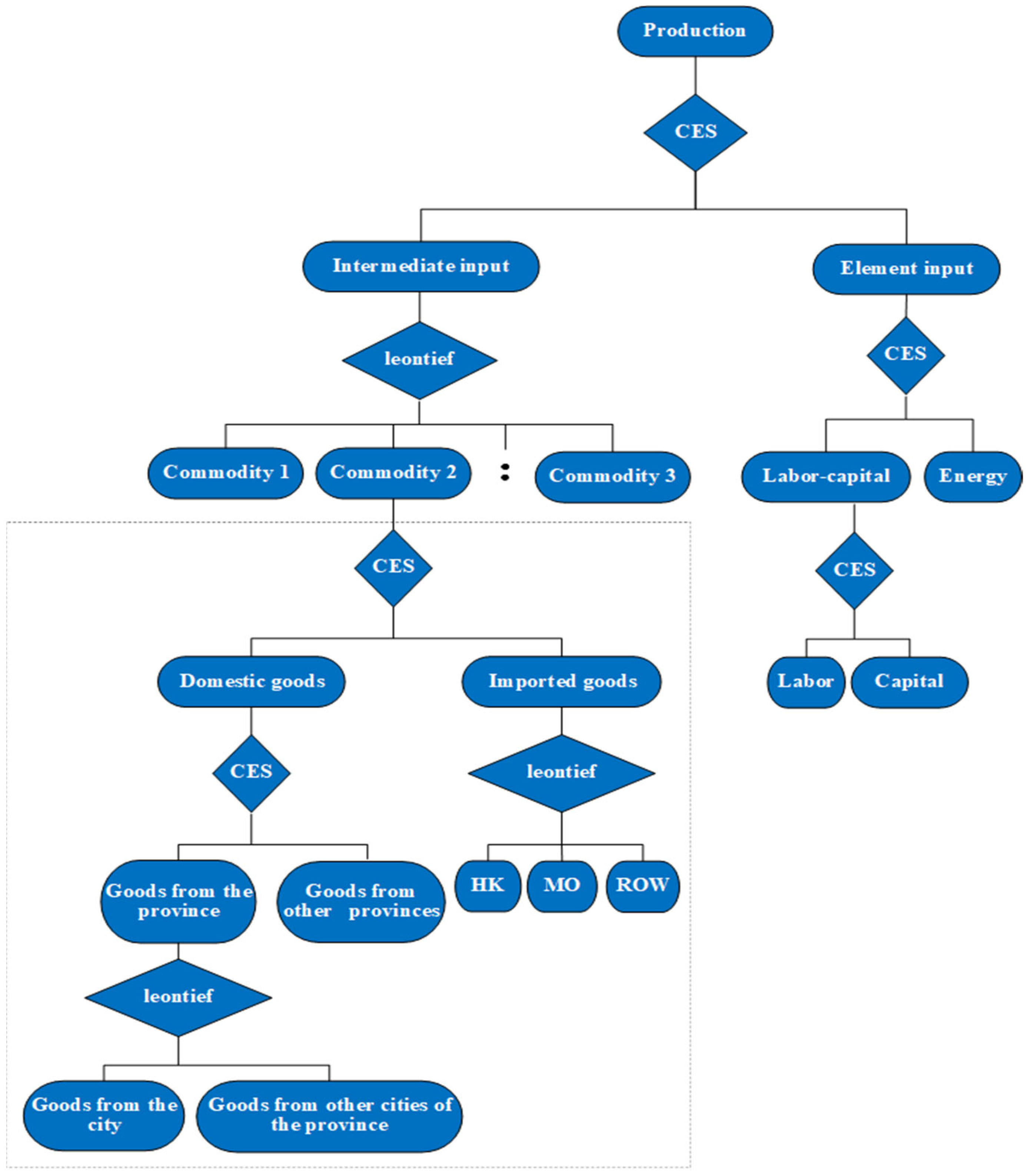
The multiregional CGE model was developed from the single-region CGE model, which includes basic production, trade, revenue and expenditure, and equilibrium modules. The optimization behavior of economic subjects occurs at the regional level, which differs from the single-region model. Thus, interregional economic relations (i.e., commodity trading, investment flows, and labor flows) must be portrayed. The GBA multiregional CGE model constructed for this study includes an optimization simulation of municipal-level economic behaviors, including 30 departments in 10 cities in the region. Economic behavior at the provincial (regional) level is also optimized by depicting the commodity trade matrix and the flow of provincial capital and labor. Hong Kong and Macao’s links with other GBA cities are reflected in the model only through commodity trade (i.e., imports and exports).

Production Modules

The production module is shown in Figure 1, where the output is a combination of the multilayer constant elasticity of substitution (CES) production or Leontief functions. The output of the first layer is a CES combination of intermediate and factor inputs. In the second layer, the intermediate input is the Leontief combination of various commodities, and the factor input is the CES combination of labor–capital combinations and energy. In the third layer, commodities include the CES combination of domestic and foreign goods, and labor–capital is the CES combination of labor and capital. In the fourth layer, domestic goods include the CES combination of goods in and out of Guangdong Province, and foreign goods are the Leontief combination of Hong Kong, Macao, and other countries. In the fifth layer, the goods in Guangdong Province are a combination of those from the specific city and other cities in the province.

Trade Module

The trade module includes two aspects: commodity buying and selling. The dotted box in Figure 1 contains the commodity buying process, and Figure 2 shows the corresponding commodity selling process. As shown, the sales of products produced by a city department contain a three-layer CES and Leontief functions. In the first layer, commodity sales are a combination of domestic and foreign sales. In the second layer, domestic sales are the CES combination of sales in and out of the province, and foreign sales are the Leontief combination exported to Hong Kong, Macao, and other countries. In the third layer, provincial sales are a Leontief combination of sales in the city and those of other cities in the province. Sales in the city must meet the intermediate needs of residents and the government, as well as the investment and inventory needs of the city.

Income and Expense Module

The income and expenditure module describes the income and consumption of residents, businesses, and governments. Resident income derives from labor remuneration, capital returns, and transfer payments (set to zero in this study), and expenditures include the consumption of goods, personal income tax payments, and deposits.

Enterprise income mainly comes from capital returns and transfer payments, and expenditures are used to pay income taxes and deposits. Government revenue includes production value-added taxes, environmental taxes, resident, and corporate income taxes, and expenditures include government consumption, deposits, and transfer payments.

Balance and Macro-Closure Modules

In commodity equilibrium, the model assumes that all commodity markets are cleared at a given price. Thus, the supply of commodities equals their demand. With macroscopic closure, model elements choose neoclassical or Keynesian closure according to the needs of the research problem. Resident consumption, government consumption, and investment demand are exogenous or endogenous, according to the problem, and commodity prices in other provinces are exogenous. Savings are endogenous, the exchange rate is exogenous, and foreign savings are endogenous.

Because this study estimates carbon prices in various cities, the cross-regional flows of labor and capital are not considered; only flows between industries within each city are considered. The flow of goods between cities is determined based on the estimated intercity trade coefficient.

2.2.2. Carbon Tax/Trading Policy Module

The task of the policy module is to link environmental and economic policies and models, which take different forms depending on policy requirements and the data-enabled situation. The collection of carbon taxes increases the enterprise cost of using fossil energy, and from the principle of cost minimization, enterprises reduce their use, thereby increasing the demand for alternatives. Carbon taxes have different degrees of impact on industries in different regions, which cause the relative prices of products in those industries to change dynamically and exert a variety of influences on product supply and demand. These influences are extended to the entire economy and society through industrial and regional linkages, affecting the decision-making of economic entities at all levels.

If a carbon tax is collected based on the amount of carbon dioxide emitted by the energy consumed by the production sector, the impact is as follows:

$$\mathrm{QE}\left(\mathrm{a}, \mathrm{n}\right)=\mathrm{QED}\left(\mathrm{a}, \mathrm{n}\right)\times \mathrm{CT}$$

(1)

$$\mathrm{PA}\left(\mathrm{a}, \mathrm{n}\right)\times \mathrm{QA}\left(\mathrm{a},\mathrm{n}\right)=\mathrm{other} \mathrm{non} \mathrm{energy} \mathrm{inputs}+\left(1+\mathrm{CT}*\mathrm{CTAX}\right)\times \mathrm{PE}\times \mathrm{QED}\left(\mathrm{a}, \mathrm{n}\right)$$

(2)

where $\mathrm{a}$ represents different production sectors, n represents different cities, $\mathrm{QE}\left(\mathrm{a},\mathrm{n}\right)$ is the quantity of carbon emissions, and $\mathrm{QED}\left(\mathrm{a},\mathrm{n}\right)$ is the energy consumed. $\mathrm{CT}$ is the carbon intensity of energy consumption (t/t), and $\mathrm{CTAX}$ is the set carbon tax rate (yuan/t). $\mathrm{PE}$ is the price of energy, $\mathrm{PA}\left(\mathrm{a},\mathrm{n}\right)$ is the price of the product, and $\mathrm{QA}\left(\mathrm{a}, \mathrm{n}\right)$ is the quantity of the product.

When a carbon trading market is introduced, two cases are considered: trading only within each region and trading between regions. In the case of trading only within each region,

$$\mathrm{PA}\left(\mathrm{a}, \mathrm{n}\right)\times \mathrm{QA}\left(\mathrm{a},\mathrm{n}\right)=\mathrm{other} \mathrm{non} \mathrm{energy} \mathrm{inputs}+\left(\mathrm{QE}\left(\mathrm{a},\mathrm{n}\right)-\mathrm{FP}\left(\mathrm{a},\mathrm{n}\right)\right)\times \mathrm{CP}\left(\mathrm{n}\right),$$

(3)

$${{\displaystyle \sum }}_{\mathrm{a}=1}^{\mathrm{r}}\mathrm{QE}\left(\mathrm{a},\mathrm{n}\right)=\mathrm{E}0\left(\mathrm{n}\right)$$

(4)

where $\mathrm{CP}\left(\mathrm{n}\right)$ is the price of pollutant discharge rights in an area, which is an endogenous variable. $\mathrm{FP}\left(\mathrm{a}, \mathrm{n}\right)$ is the number of pollutant discharge rights (t) issued free of charge in an industry, which is an exogenous variable. $\mathrm{E}0\left(\mathrm{n}\right)$ is the allowable carbon emissions (t) set for exogenous emissions based on emissions reduction targets, and r is the total number of trade industries.

In the case of trading only between regions,

$$\mathrm{PA}\left(\mathrm{a}, \mathrm{n}\right)\times \mathrm{QA}\left(\mathrm{a},\mathrm{n}\right)=\mathrm{other} \mathrm{nonenergy} \mathrm{inputs}+\left(\mathrm{QE}\left(\mathrm{a}, \mathrm{n}\right)-\mathrm{FP}\left(\mathrm{a}, \mathrm{n}\right)\right)\times \mathrm{CP},$$

(5)

$${{\displaystyle \sum }}_{\mathrm{n}=1}^{\mathrm{N}} {{\displaystyle \sum }}_{\mathrm{a}=1}^{\mathrm{r}}\mathrm{E}\left(\mathrm{a},\mathrm{n}\right)=\mathrm{E}0$$

(6)

where $\mathrm{CP}$ is the price of pollutant discharge rights for the whole region and is an endogenous variable. $\mathrm{E}0$ is the region-wide carbon permissible emissions (t) set for exogeneity based on emissions reduction targets, and $\mathrm{N}$ is the total number of trading areas.

2.3. Parameter Setting and Model Validation

Based on the SAM table of each city in the base year (2017), various parameters (e.g., scale coefficient, share coefficient, value-added tax rate, individual income tax rate, corporate income tax rate, and residents’ consumption tendency) are estimated. The substitution elasticity data in the model are empirically valued, as shown in

Table A1. Substitution elasticity coefficients in the model.

Parameters	Values	Description
$\mathrm{rh}0\mathrm{Aa}\left(\mathrm{a},\mathrm{n}\right)$	0.3	Substitution elasticity of intermediate input and labor-capital bundle
$\mathrm{rh}0\mathrm{VA}\left(\mathrm{a},\mathrm{n}\right)$	0.2	Substitution elasticity of labor-capital bundle
$\mathrm{rh}0\mathrm{EVA}\left(\mathrm{a},\mathrm{n}\right)$	0.2	Substitution elasticity of energy&labor-capital bundle
$\mathrm{rh}0\mathrm{Qq}\left(\mathrm{c},\mathrm{n}\right)$	0.6	Substitution elasticity of domestic commodity and import commodity under the Armington condition.
$\mathrm{rh}0\mathrm{CET}\left(\mathrm{c},\mathrm{n}\right)$	1.4	Substitution elasticity of domestic commodity and export commodity in the CET function.

. The sensitivity analysis of these elasticity coefficients shows that their values have little effect on the results.

The simulated values of some key variants are compared to real values in the base year (2017), as shown in

Table A2. Base year equilibrium test (10⁸ yuan).

		GDP	Government Revenue	Resident Income	Enterprise Income	Imports	Transfer-in	Provincial Supply	Exports	Transfer-out
G Z	simulated	19,957	3099	9374	5200	3921	11,221	4173	5792	8240
	real	19,955	3099	9373	5200	3923	11,226	4166	5794	8249
S Z	simulated	21,621	3176	10,643	5402	11,512	16,656	5133	16,590	13,781
	real	21,581	3170	10,622	5392	11,473	16,621	5131	16,528	13,744
Z H	simulated	2594	413	1245	667	1109	2334	252	1887	1609
	real	2590	413	1243	666	1107	2331	251	1883	1606
F S	simulated	9633	1563	4382	2635	1214	9509	545	3196	8408
	real	9579	1554	4357	2620	1204	9459	559	3155	8338
H Z	simulated	3884	648	1925	933	1187	4211	1300	2238	4084
	real	3871	646	1918	930	1183	4201	1297	2233	4064
D W	simulated	8276	1258	4105	2036	5297	6323	130	6984	7020
	real	8324	1266	4129	2047	5328	6354	125	7027	7073
Z S	simulated	3076	464	1477	790	529	3790	88	2074	2523
	real	3059	462	1469	786	526	3768	87	2056	2505
J M	simulated	2504	381	1250	612	308	3494	664	1068	2751
	real	2514	383	1255	615	309	3509	669	1076	2770
Z Q	simulated	2173	304	1146	513	135	2650	230	223	2344
	real	2172	304	1145	513	136	2649	229	222	2341
O T	simulated	15,006	2236	8014	3313	7124	8620	7448	4837	9420
	real	15,002	2235	8011	3312	7122	8619	7448	4836	9416

. The verification results show that the model accurately reproduces the situation in the base year and can be used for the simulation and analysis of GBA environmental economic policies. The main code and model description are shown in Appendix B.

3. Analysis and Discussion

3.1. Scheme Settings

According to the Nationally Determined Contribution Plan [7], China’s carbon dioxide emissions will peak around 2030, and carbon dioxide emissions per unit of GDP will be reduced by 60–65% compared with 2005. To this end, Guangdong Province actively responded to the call of the country and clarified its 14th Five-Year Plan [8], in which its energy consumption per unit of GDP will be decreased by 18%. Although the overall target for carbon emissions reduction has been determined, the planning period is still in effect, and the macroeconomic situation of the social economy and development level of energy technology are not yet clear. Thus, it is necessary to analyze and discuss the important influencing factors of carbon prices from multiple perspectives.

The prediction scheme was considered based on the following dimensions. First, reduction intensity was used to examine the carbon price and socioeconomic impact of each city under different emissions reduction requirements. Second, the model’s macro-closure setting was used to examine the different effects of carbon emissions reduction on the prediction results under different economic situations. Third, energy replaceability was used to analyze the effects of the development of energy technology on the prediction results. See the description in

Table 2. Prediction scheme.

Reduction intensity	s1: The emissions reduction rate of each city is 3%, representing the average annual emissions reduction intensity under the emissions reduction target. s2: The emissions reduction rate of each city is 5%, representing the situation of high emissions reduction intensity in a year. s3: The emissions reduction rate of each city is 10%, representing a situation in which the intensity of emissions reduction is very high in a year.
Substitution elasticity	ρ1 = 0.1; ρ2 = 0.2; ρ3 = 0.3.
Macro-closure	c1: Neoclassical macro-closure: The quantity of labor and capital is exogenous, and the price is endogenous; the quantity of energy is exogenous, and the price is endogenous. c2: Keynes closure; labor and capital prices are exogenous, set to 1, and the quantity is endogenous; The quantity of energy is exogenous, and the price is endogenous.

.

3.2. Analysis of Results

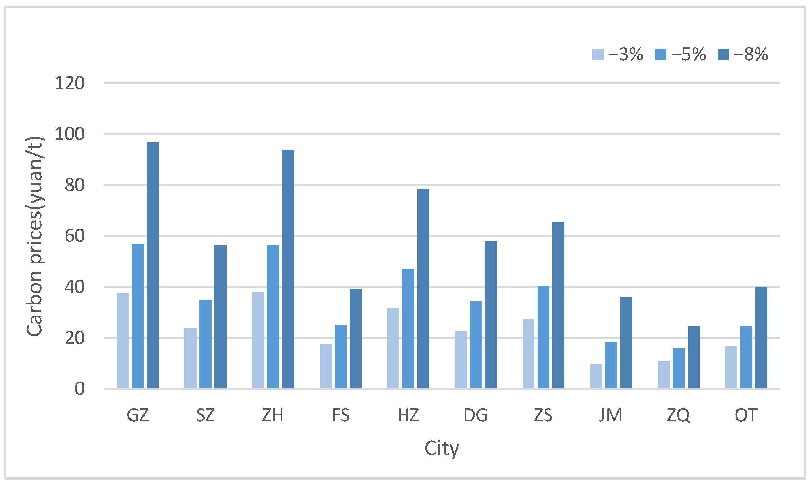
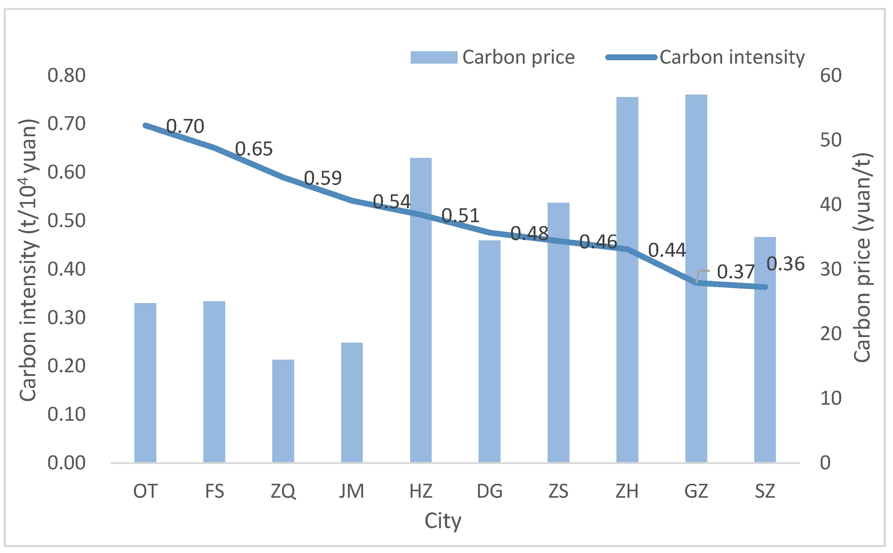
3.2.1. Characteristics of Carbon Emissions Reduction Costs (i.e., Carbon Prices) in Each City

Using the multiregional CGE model established above, the cost or price of carbon reduction in each city was calculated under each city’s emissions reduction target. The results are shown in Figure 3.

As shown in Figure 3, the level of a city’s carbon price or the carbon tax that should be levied is related to the reduction target, and the larger the reduction rate, the higher the carbon price.

When the reduction rate increases from 3% to 8%, the carbon price increases from 37 to 97 yuan/t in Guangzhou, 24 to 56 in Shenzhen; 38 to 94 in Zhuhai, 18 to 39 in Foshan, 32 to 78 in Huizhou, 23 to 58 in Dongguan, 27 to 65 in Zhongshan, 10 to 36 in Jiangmen, 11 to 24 in Zhaoqing, and 17 to 40 in other cities.

Additionally, the carbon price of each city differs, indicating that it also depends on the characteristics of the city’s economy (e.g., industrial and trade structures), and the relationship between the carbon price and its emission intensity can be roughly analyzed, as shown in Figure 4.

The relationship between carbon price and intensity can be seen in Figure 4. Essentially, the higher the carbon intensity, the lower the carbon price, and the two show a reverse trend. Other cities (cities excluding the nine cities in GBA), Jiangmen, Zhaoqing, and Foshan have higher carbon intensities, averaging about 0.61 t/10⁴ yuan, with a low carbon price averaging about 21 yuan/t. Guangzhou, Shenzhen, Zhuhai, Huizhou, Dongguan, and Zhongshan have an average carbon intensity of about 0.44 t/10⁴ yuan, with an average carbon price of 45 yuan/t. Although not statistically negatively correlated, this trend is evident. This reveals that relatively clean cities with lower carbon intensities are less sensitive to carbon prices and require higher prices to meet emissions reduction targets, and thus the direct cost of emissions reduction is higher. Whereas relatively unclean cities with higher carbon intensities are more sensitive to carbon prices, so lower carbon prices can achieve emissions reduction targets and the direct cost of emissions reduction is relatively low.

Therefore, we must next determine whether we give more reduction tasks to cities with lower direct reduction costs and how emission reductions affect city economies. We must also calculate the opportunity costs of carbon reduction for each city. Next, the economic impact of emissions reductions on each city is analyzed at both macroscopic and microscopic levels.

3.2.2. Economic Impact of Carbon Emissions Reduction on Each City

Macroeconomic Impact

The macroeconomic impacts of a 5% reduction in carbon emissions on each city are shown in

Table 3. Impact of carbon dioxide emissions reduction on the macroeconomy (5% emissions reduction in each city, unit: %).

City	QA	GDP	QDAL	QDAP	QE	QDCL	QDCP	QM	YG	QH
GZ	−0.69	−0.22	−0.65	−1.05	−0.72	−0.77	−0.60	−0.62	−0.49	−0.08
SZ	−0.42	−0.11	−0.47	−0.44	−0.40	−0.46	−0.54	−0.27	−0.32	−0.31
ZH	−0.45	−0.10	−0.43	−0.38	−0.42	−0.43	−0.14	−0.99	−0.52	−0.28
FS	−0.66	−0.24	−0.66	−0.66	−0.11	−0.68	−0.48	−0.20	−0.56	−0.51
HZ	−0.42	−0.16	−0.39	0.15	−1.36	−0.33	−0.80	0.40	−0.76	−0.27
DG	−0.09	0.14	−0.16	0.20	−0.50	−0.11	−0.42	−0.10	−0.09	−0.07
ZS	−0.51	−0.12	−0.53	−0.55	0.08	−0.53	−0.31	−0.02	−0.37	−0.35
JM	−0.15	0.28	−0.22	0.21	0.22	−0.13	0.02	0.13	−0.10	0.00
ZQ	−0.53	−0.05	−0.51	−0.42	−0.36	−0.52	−0.41	−0.20	−0.41	−0.28
OT	−0.58	−0.07	−0.51	−0.42	−0.11	−0.50	−0.37	−0.39	−0.77	−0.29

QA (output); QDAL (local demand); QDAP (transfer out); QE (export); QDCL (provincial supply); QDCP (transfer in); QM (import); YG (government revenue); QH (resident consumption).

.

Table 3 shows that under the constraint of the same carbon emissions reduction rate (5%), the total social output value of each city is reduced by varying degrees (−0.09 to −0.69%). The GDP in most cities has some degree of reduction (−0.05 to −0.24%), but Dongguan (+0.14%) and Jiangmen (+0.28%) increase slightly.

In the context of carbon reduction, owing to the impact of the implied carbon price, the production costs of most industries increase, especially in high-carbon industries. However, there are also some low-carbon industries whose production costs decrease due to the depreciation of labor and capital, owing to the relative abundance. Changes in production costs in different industries lead to changes in supply and demand. Overall, local demand in each city decreases (−0.16 to −0.66%), as does the demand outside the province (−0.38 to −1.05%). Foreign demand also decreases (−0.11 to −1.36%), except in Huizhou, Dongguan, and Jiangmen. From the supply perspective, the supply from the province (−0.11 to −0.77%), from other provinces (−0.14 to −0.80%), and from foreign sources (−0.02 to −0.99%) all decrease, apart from a few cities.

Government revenue is also affected (−0.09 to −0.76%) due to the reduction of total social output, and residential consumption decreases (−0.07 to −0.51%), except in Jiangmen.

The above predictions assume that the socioeconomic situation is under neo-classically closed conditions, in which the quantity of labor and capital is fixed, and carbon emissions reduction targets are met by limiting the amount of energy used. Under such macro-closure conditions, the overall impact of carbon emissions reduction on the social economy of each city is relatively small, but the macroeconomic indicators of the cities show different characteristics due to their different industrial and trade structures, which are explained in detail from the perspectives of the industries.

Microeconomic Impact

The impact of carbon reductions on each city’s sectors is shown in Figure A1. Using Figure A1 and the IO data of each city decomposed above, the main production and trade industries in each city and the most and least affected sectors are listed in the following

Table 4. Economic impact of carbon emissions reduction on various sectors in each city.

City	Output		Trade		Most Affected		Less Affected
	Sector	Ratio (%)	Sector	Ratio (%)	Sector	Ratio (%)	Sector	Ratio (%)
GZ	OTS	34.86	TRE	29.01	EPHP	−6.3	SWAT	−0.3
	WRHR	12.63	WRHR	17.46	SGAS	−6.21	OTS	−0.17
	TRE	10.91	CEC	6.79	PCN	−4.52	CNS	−0.07
	CNS	7.84	NMM	6.4	MINE	−1.99	FOOD	−0.03
	CMC	5.11	MPR	4.6	TRE	−1.26	AGRI	0.05
SZ	CEC	31.69	CEC	43.84	EPHP	−7.51	SPP	−0.2
	OTS	26.65	CMC	11.34	SGAS	−7.07	OTS	−0.2
	WRHR	7.78	WRHR	9.35	PCN	−4.5	CNS	−0.07
	CNS	5.57	EME	5.45	MINE	−1.66	FOOD	0.03
	EME	4.54	FOOD	4.3	TXT	−1.35	AGRI	0.18
ZH	OTS	21.17	EME	23.44	SGAS	−6.5	WRHR	−0.05
	CEC	11.99	CEC	22.7	PCN	−6.47	GEP	0
	CNS	11.7	WRHR	10.06	EPHP	−5.77	SPP	0.01
	EME	10.53	PCN	6.55	MINE	−1.88	EME	0.04
	CMC	8.97	NMM	6.37	TXT	−1.1	CEC	0.31
FS	OTS	14.56	EME	36.98	EPHP	−7.46	GEP	−0.12
	EME	14.41	CEC	10.8	SGAS	−7.22	CEC	−0.11
	MPR	8.45	MPR	9.71	PCN	−4.81	SPP	−0.08
	CMC	7.87	PPC	8.79	TXTG	−2.46	TRE	−0.07
	SPM	6.02	TRE	5.84	TXT	−1.83	EME	0.01
HZ	CEC	29.06	CEC	29.62	SGAS	−6.52	I&M	0.08
	OTS	14.57	OTS	16.22	EPHP	−6.14	GEP	0.08
	CMC	9.19	TXTG	13.28	PCN	−4.85	SPP	0.16
	WRHR	6.76	EME	6.78	TXT	−3.71	EME	0.32
	EME	4.69	FOOD	6.21	TXTG	−3.66	CEC	1.08
DG	CEC	30.91	CEC	25.44	SGAS	−6.73	GEP	0.1
	OTS	16.31	EME	10.27	EPHP	−6.61	NMM	0.15
	WRHR	6.43	GEP	9.94	PCN	−4.42	SPP	0.33
	PPC	6.4	TSP	8.45	TXT	−2.72	EME	0.39
	CMC	5.32	CMC	6.84	TXTG	−2.58	CEC	1.18
ZS	OTS	22.63	EME	41.44	SGAS	−6.79	SPP	−0.08
	EME	12.57	CEC	10.17	EPHP	−6.36	FOOD	−0.04
	CEC	9.63	TXTG	5.4	PCN	−4.44	GEP	0
	CMC	8.12	FOOD	4.85	TXT	−2.25	EME	0.14
	WRHR	7.24	WRHR	4.8	TXTG	−1.99	CEC	0.16
JM	OTS	18.79	CEC	19.92	SGAS	−6.86	GEP	0.4
	MPR	8.49	MPR	11.06	EPHP	−6.18	SPM	0.41
	FOOD	7.71	EME	10.38	PCN	−4.45	MNF	0.42
	CMC	6.53	AGRI0	8.58	MINE	−1.04	TRE	0.74
	EME	6.18	GEP	7.1	TXTG	−0.8	EME	0.84
ZQ	OTS	18.5	MPR	18.98	EPHP	−7.06	SPP	−0.04
	MPR	11.2	GEP	16.74	SGAS	−6.96	CEC	−0.04
	AGRI	8.44	FOOD	12.89	PCN	−4.86	WRHR	−0.03
	WRHR	7.81	TSP	10.15	MINE	−1.36	AGRI	−0.02
	NMM	7.66	WRHR	7.62	TSP	−1.24	FOOD	0.31

for convenience of analysis.

Guangzhou (GZ)

From Table 4, the top three industries in Guangzhou all have low carbon footprints with the services (30), wholesale and retail (29), and transportation equipment industries (18) accounting for more than 50% of the output. The top three major trade industries also have low carbon footprints, and the top two are the leading industries in Guangzhou, accounting for more than 45% of trade. Industries with a greater impact caused by carbon reduction are the energy sectors (i.e., power (24), gas (25), petroleum coking (11), and kerosene mining (2–5)), and the transportation equipment (18) industry (i.e., the top trade sector). An industry that benefits from carbon emissions reduction is the agricultural sector (1), showing a slight increase of 0.05% in its output value.

A large impact of carbon reductions is expected on the high-carbon energy sector, but the impact on the low-carbon sectors (e.g., transportation equipment (18)) requires further examination. Interestingly, the sector price change (1.00087) increases under carbon emissions reductions, which suppresses local (−1.14%), out-of-province (−1.50%), and foreign demand (−1.50%). Because this sector is trade intensive, the reduction in demand is much greater than those with small trade, resulting in a large reduction in output (−1.26%).

The output of the agricultural sector (1) increases by 0.05%, and both labor and capital shift to the sector, increasing by 0.10 and 0.64%, respectively. Local consumption decreases by 0.09%, and imports and provincial transfers-in decrease by 0.15%. However, provincial transfers out and exports increase by 0.04%. Although carbon price increases some production costs in the agricultural sector (1), owing to the relative enrichment of labor and capital and the relatively depreciated value, the price change (0.9992) is relatively low compared with prices outside the province and globally. Thus, it is conducive to transfers out and exports.

In summary, Guangzhou is a relatively clean city with a low carbon intensity (0.37 t/10⁴ yuan) and relatively high carbon prices (57 yuan/t), and the GDP loss induced by carbon emissions reduction (−5%) is 0.22%, which is comparatively large among the nine cities.

Shenzhen (SZ)

The top three industries in Shenzhen are also low-carbon industries (i.e., computers (20), services (30), and wholesale and retail (29)), and the industrial output value accounts for more than 60%. The main trade industries have mostly low carbon footprints, apart from the chemical industry (12), which accounts for more than 60% of trade. In addition to the energy sector, the textile sector (7) is among the top five most affected. Industries benefitting from carbon reduction include agricultural (1) and food and tobacco (6), with output values increasing by 0.18 and 0.03%, respectively.

Notably, the computer industry (20) is the largest in Shenzhen (31.69%) and the largest in trade (43.84%). However, it is not greatly affected, unlike the transportation equipment sector (18) in Guangzhou. The main reason for this is that the depreciation of labor and capital offsets the impact of carbon prices, leaving the sector price largely unchanged (0.9999); hence, demand is less affected.

The carbon intensity of Shenzhen (0.36 t/10⁴ yuan) approximates that of Guangzhou. However, under the same reduction rate (−5%), the carbon price (35 yuan/t) is lower than that of Guangzhou (57 yuan/t), indicating that, in addition to carbon intensity, carbon prices are also related to other factors, such as industrial and trade structures. Because the main industries affected by carbon emissions reduction have high carbon footprints, Shenzhen is more sensitive to carbon prices, and the price required to achieve the same reduction rate is lower than that of Guangzhou. Notably, the economic impact of carbon emissions reduction is medium (−0.11%).

Zhuhai (ZH)

There are three low-carbon industries among the top five in Zhuhai (i.e., services (30), computers (20), and electrical machinery (19)), and their outputs account for more than 40% of the total. The top three major trade industries also have low carbon footprints (electrical machinery (19), computers (20), and wholesale and retail (29)), accounting for more than 50% of trade. The industries most affected by carbon emissions reduction all have high carbon footprints, and those benefitting from carbon prices include computers (20) and electrical machinery (19), with their output values increasing by 0.31 and 0.04%, respectively.

Computers (20) and electrical machinery (19) industries are not only the main output sectors in Zhuhai, but they are also the main trade sectors that benefit from carbon emissions reduction. The increased carbon price, combined with depreciated labor and capital, leads to a slight decrease in the prices of these two sectors: 0.9999 and 0.9994, respectively. The reduction in prices increases demand, stimulates production, and increases carbon emissions to an extent. Zhuhai’s industrial and trade structures make it less sensitive to carbon prices. Although its carbon intensity (0.44 t/10⁴ yuan) is higher than that of Guangzhou, it maintains a similar carbon price (57 yuan/t). Moreover, carbon emissions reduction has a medium impact on the economy (−0.10%).

Foshan (FS)

Three of Foshan’s top five industries have medium or high carbon footprints (i.e., metal products (15), chemical (12), and metal smelting (14)), with a carbon intensity (0.65 t/10⁴ yuan) higher than the previous three cities. Two medium-carbon industries are among the main trade sectors (metal products (15) and paper printing (10)). In addition to the high-carbon sector (i.e., energy), there are low-carbon sectors (e.g., textile and products industry (8)) that are affected by carbon reduction. The industries with less impact include low-carbon industries (i.e., electrical machinery (19) and transportation equipment (18)).

The main reason for the impact on low-carbon textile and products industries (8) is similar to that of the transportation equipment sector (18) in Guangzhou; that is, it is the second largest trade sector in Foshan, and the increase in carbon prices causes the prices of products to rise (1.0019), resulting in a reduction in demand from abroad and from outside the province. Thus, there was a greater reduction in output (−2.46%).

Foshan’s medium- and high-carbon industries account for a significantly higher proportion than the other three cities, and because carbon emissions reductions have a greater impact on those, Foshan is sensitive to carbon prices. Thus, it requires a comparatively low price (25 yuan/t). However, the impact of carbon reduction on its economy is the largest (−0.24%) among all cities. Although the direct emissions reduction cost of Foshan is low, the opportunity cost is high, which is a problem that needs to be balanced by the smart allocation of carbon quotas.

Huizhou (HZ)

Among the top five industries in Huizhou, four have low carbon footprints, and their industrial output value accounts for more than 50% of the total. The main trade industries are also low carbon, accounting for more than 70% of trade. In addition to the high-carbon energy sector, the textile and products industry (8) is also largely affected by carbon emissions reduction, and the reasons are like those of Foshan and Guangzhou. Industries that benefit from carbon emissions reduction all have low carbon footprints (e.g., computers (20) and electrical machinery (19)).

Huizhou’s carbon intensity is 0.51 t/10⁴ yuan, and the industrial and trade structures are similar to those of Zhuhai, whose pillar industry (29.06%) is computers (20), which is also the main trade industry (29.62%). It clearly benefits from carbon emissions reduction. Therefore, Huizhou is also less sensitive to carbon prices and has a relatively high value of 47 yuan/t, and the economic impact of carbon emissions reduction is medium (−0.16%).

Dongguan (DG)

The top three industries in Dongguan have low carbon footprints, with industrial output accounting for more than 50% of the total. However, medium- and high-carbon industries (i.e., paper printing (10) and chemical (12)) account for a considerable proportion. Among the main trade industries, the top three have low carbon footprints, accounting for 45% of trade, and high-carbon industries (i.e., transportation (28) and chemical (12)) account for a lot. The industries most affected by carbon emissions reduction are high-carbon sectors, but low-carbon textile and product sectors (8) are also impacted. The industries that benefit from carbon emissions reductions include those with low carbon footprints (i.e., computers (20), electrical machinery (19), and special equipment (17)).

The carbon intensity of Dongguan is 0.48 t/10⁴ yuan, and its industrial and trade structures are like those of Zhuhai and Huizhou. However, because high-carbon industries account for a good proportion of its main production and trade, Dongguan is more sensitive to carbon prices than Zhuhai or Huizhou, and the carbon price (34 yuan/t) is lower than those cities. However, because many industries benefit from carbon emissions reduction, Dongguan’s GDP increases slightly (0.14%).

Zhongshan (ZS)

There are four low-carbon industries in Zhongshan’s top five, with an industrial output value of more than 50% of the total. The top five trade industries all have low carbon footprints, accounting for more than 65% of trade. The most affected industries are the high-carbon energy sector and the low-carbon textiles and products (8) sectors. The industries that benefit from carbon emissions reduction are those with low carbon footprints (i.e., computers (20) and electrical machinery (19)).

Zhonghan’s industrial and trade structures are like those of Huizhou, and the economic volume, carbon intensity (0.46 t/10⁴ yuan), and carbon price (40 yuan/t) all approximate those of Huizhou. The economic impact of carbon emissions reduction is medium (−0.12%).

Jiangmen (JM)

Jiangmen’s top five industries have medium carbon footprints. There are also two medium-carbon industries in the main trade category, and the most affected are the high-carbon energy and the low-carbon textile and products industries (8). Low-carbon industries (i.e., electrical machinery (19) and transportation equipment (18)) benefit, as does the high-carbon metal smelting industry (14).

To determine why carbon emissions reductions have little negative or even positive impact on the high-carbon metal smelting industry (14), an analysis of the production and trade in the city was performed. The consumption demand for this sector mainly comes from the intermediate production of Jiangmen, and the supply mainly comes from other provinces and local production. Moreover, carbon reductions induce only a small increase in the production cost of this sector (1.00033), so the demand is not much affected. In addition, because Jiangmen is not trade intensive, the impact of carbon emissions reduction on most of its industries is not as great as other trade-intensive cities. Overall, Jiangmen’s GDP increases, thereby increasing the intermediate demand for the industry, and the output of the sector increases (0.41%).

Medium-carbon industries account for a relatively large proportion of business in Jiangmen. Thus, its carbon intensity (0.54 t/10⁴ yuan) is high. Therefore, the city is sensitive to carbon prices, and the direct reduction cost (18.6 yuan/t) is relatively low. The opportunity cost of carbon emissions reduction is also small, and the GDP increases (0.28%). However, special consideration should be given to sectors that suffer greatly, such as the high-carbon energy and the low-carbon trade-intensive sectors.

Zhaoqing (ZQ)

The top five industries of Zhaoqing include two with medium- and high-carbon footprints (i.e., metal products (15) and non-metallic mineral products (13)). Among the top five trade industries, two have medium and high-carbon footprints (i.e., metal products (15) and transportation (28)). The most affected are the high-carbon energy and transportation sectors (28). Notably, the low-carbon food and tobacco sectors benefit.

The medium- and high-carbon industries of Zhaoqing account for a large proportion, and the city’s carbon intensity (0.59 t/10⁴ yuan) is high. Therefore, Zhaoqing is sensitive to carbon prices and has a low carbon price (16 yuan/t). The economic impact of carbon emissions reduction is small (−0.05%).

3.2.3. Comparison with Related Studies

Relatively few studies have applied the CGE model to calculate the cost of carbon reduction at the city level, but some provincial carbon reduction cost studies have been carried out. For example, Yuan et al. [25] used a multiregional CGE model to calculate provincial carbon prices under a 10% reduction in emissions reduction intensity over the baseline year covering industries of steel, non-ferrous, building materials, petroleum processing, chemical and thermal power generation, and other emission sources. The carbon emission price in Guangdong was found to exceed 110 yuan/t. Wang et al. [16] used a two-region dynamic CGE model to calculate the carbon price of Guangdong Province required to achieve Copenhagen emissions reduction targets. Note that China pledged to reduce its CO₂ emission intensity per unit GDP by 40–45% by 2020 compared with 2005 levels. The sector order of carbon prices from low to high was found to be cement, electricity, refining, and steel, and the carbon price in the power industry was relatively stable at 107–194 yuan/t. As found by Tang et al. [19], when the emissions reduction sector includes only the power industry, the carbon price needed to meet the emissions reduction target was 60 yuan/t in 2020 and will be 1140 yuan/t by 2030. When multiple sectors of power, chemical, nonferrous metals, paper, ferrous metals, nonmetallic mineral products, petroleum processing, and transportation are included, the carbon price was 26 yuan/t in 2020 and will be 345 yuan/t in 2030.

This study involved all industry sectors in carbon emissions reduction, and the target was a 5% reduction in carbon intensity over the baseline year. Compared with the aforementioned studies covering only high-carbon industries, the carbon prices found in this study are relatively low, which is also reasonable.

Some scholars have also calculated the cost of carbon reduction at the city level by using the shadow price model. For example, Wang et al. [13] used a data envelopment analysis (DEA)-based method to evaluate the regional CO₂ shadow prices of 30 Chinese major cities. They found that the average industrial CO₂ emissions abatement cost was 45 $/t during the period 2006–2010 and a large gap on CO₂ shadow prices existed between different Chinese regions, with the price of 170.70 $/t in the east coast area and 6.32 $/t in the middle Yellow River area. Yang et al. [14] applied a parameterized directional distance function approach to estimate the regional CO₂ marginal abatement costs in China based on provincial panel data covering the years 2003–2012 and calculated the average shadow prices of CO₂ as 717.27 yuan/t for the whole country. The east coast and south coast areas have the highest shadow prices of CO₂ (1143.48 yuan/t and 1088.26 yuan/t, respectively), and the northwest area has the lowest shadow price (336.18 yuan/t).

It should be noted that the cost of emission reductions calculated by the shadow price model is an opportunity cost, as described earlier. This method cannot be used to simulate policy changes; only historical emission reduction costs can be calculated. It also lacks sectoral dynamic interaction paths and technical implications. From the calculation results, most of the opportunity costs are much larger than the actual carbon market price, while the direct emission reduction cost calculated by the CGE model is closer to the carbon market price.

Although the CGE model can calculate the cost of carbon emission reductions more comprehensively, it should also be noted that it does not pay attention to the details of emission reduction technology, which is also the direction in which the model should be improved in the future.

3.3. Uncertainty Analysis

3.3.1. Impact of Energy–Labor and Capital Substitution Elasticity

In the model of this study, the energy–labor and capital substitution elasticity parameter was set to 0.2. For the uncertainty analysis, this parameter was increased or decreased by 50% to observe the influences of the substitution elasticity coefficient on the important model results and their economic significance, as shown in

Table 5. Impact of substitution elasticity on gross domestic product (GDP) and carbon price.

City	ρ = 0.2		ρ = 0.3		ρ = 0.1
	GDP (108 yuan)	Carbon Price (yuan/t)	GDP Change (%)	Carbon Price Change (%)	GDP Change (%)	Carbon Price Change (%)
GZ	19,907.72	57.02	0.026	−8.26	−0.024	7.66
SZ	21,578.51	34.96	0.001	−7.75	−0.001	7.24
ZH	2589.13	56.63	0.003	−9.48	−0.003	8.93
FS	9576.98	25.00	0.001	−8.21	−0.001	7.72
HZ	3868.37	47.21	0.004	−9.49	−0.003	8.89
DG	8322.83	34.45	0.001	−9.27	−0.001	8.60
ZS	3059.12	40.27	0.001	−8.93	−0.001	8.39
JM	2513.42	18.59	0.001	−10.99	−0.001	10.36
ZQ	2171.55	15.99	0.001	−5.40	−0.001	5.05
OT	14,992.86	24.71	0.003	−7.67	−0.003	7.19

.

As shown in Table 5, the change in substitution elasticity has little impact on GDP. When the elasticity coefficient increases by 50%, the maximum GDP change decreases by 0.026%. When the elasticity coefficient decreases by 50%, the maximum GDP change increases by 0.024%. From these results, we can draw two main conclusions. First, substitution elasticity has less of an effect on the absolute value of GDP. Second, its increase reduces the impact of carbon reduction on GDP. Thus, the social (opportunity) cost of carbon reduction can be reduced.

Although the substitution elasticity of energy has a small impact on GDP, it has a modest impact on carbon price. When the elasticity coefficient increases by 50%, the maximum decrease in the carbon price is 10.99%. When it decreases by 50%, the maximum increase in the carbon price is 10.36%. This shows that with the increase of substitution elasticity, the carbon price in various cities decreases, namely the direct cost of carbon emissions reduction is reduced.

3.3.2. Analysis of the Influence of Macroscopic Closure Conditions

Carbon prices are affected by the closure conditions of the model. Under neoclassical closure conditions, the industrial structure is adjusted under the background of carbon reduction, for which high-carbon industries are inhibited, low-carbon industries relatively benefit, and the overall social economy is less affected. The overall carbon price is related to carbon intensity, the higher the carbon intensity, the lower the carbon price. This proposition was confirmed for Foshan, Zhaoqing, and Jiangmen with high carbon intensities and low carbon prices. Guangzhou and Zhuhai have low carbon intensities and high carbon prices. Additionally, the cities’ trade structures impact carbon prices, and those with large trade volumes are more sensitive, such as Shenzhen and Dongguan. Although they have low carbon intensities, they also have relatively low carbon prices compared with other cities with the same carbon intensities.

During a social economic depressed situation, some capital is idle, the labor force is not fully employed, and the social economy is demand driven. Hence, the implementation of carbon emissions reduction has a greater impact on the entire social economy, and all industries are greatly affected. See Figure 5.

Figure 5 shows that, under Keynesian closure conditions, GDP losses are much larger than those in the neoclassical closure condition. That is, a 5% emissions reduction rate causes a GPD loss of 2.11–5.05% per city. We can see that carbon prices are negatively correlated with the degree of economic impact. Thus, the greater the affected degree of the cities (e.g., Foshan, Dongguan, Huizhou, and Zhongshan), the lower the carbon price.

4. Conclusions and Suggestions

Using the IO table and socioeconomic data of Guangdong Province from 2017, this paper decomposed various statistical data into city and industry by RAS and other methods to obtain the multiregional IO tables of nine cities in the GBA. Thus, a multiregional CGE model of Guangdong Province was established. By linking the carbon emissions reduction policy variables to the model, the policy simulation scheme for different emissions reduction intensities was established according to the carbon emission target of Guangdong Province, and the carbon emission reduction costs (carbon price/tax needed for each city) to achieve emissions reduction targets were calculated. The conclusions are as follows:

• The carbon price of each city is positively correlated with the intensity of emissions reduction but is negatively correlated with the carbon intensity. Meanwhile, the carbon price of each city is affected by its own industrial and trade structure. Cities with high carbon intensity (e.g., Zhaoqing, Jiangmen, and Foshan) are sensitive to carbon prices (i.e., low carbon prices lead to low direct emissions reduction costs). Otherwise, cities with low carbon intensities (e.g., Guangzhou, Shenzhen, Zhuhai, Huizhou, Dongguan, and Zhongshan) are relatively insensitive to carbon prices (i.e., relatively high carbon prices lead to high direct emissions reduction costs when the same emissions reduction is reached). Additionally, the intensity of trade also has a certain impact on carbon prices. Cities with large trade volumes are more sensitive to carbon prices because they increase the cost of products and have a greater impact on supply and demand (e.g., Shenzhen and Dongguan).
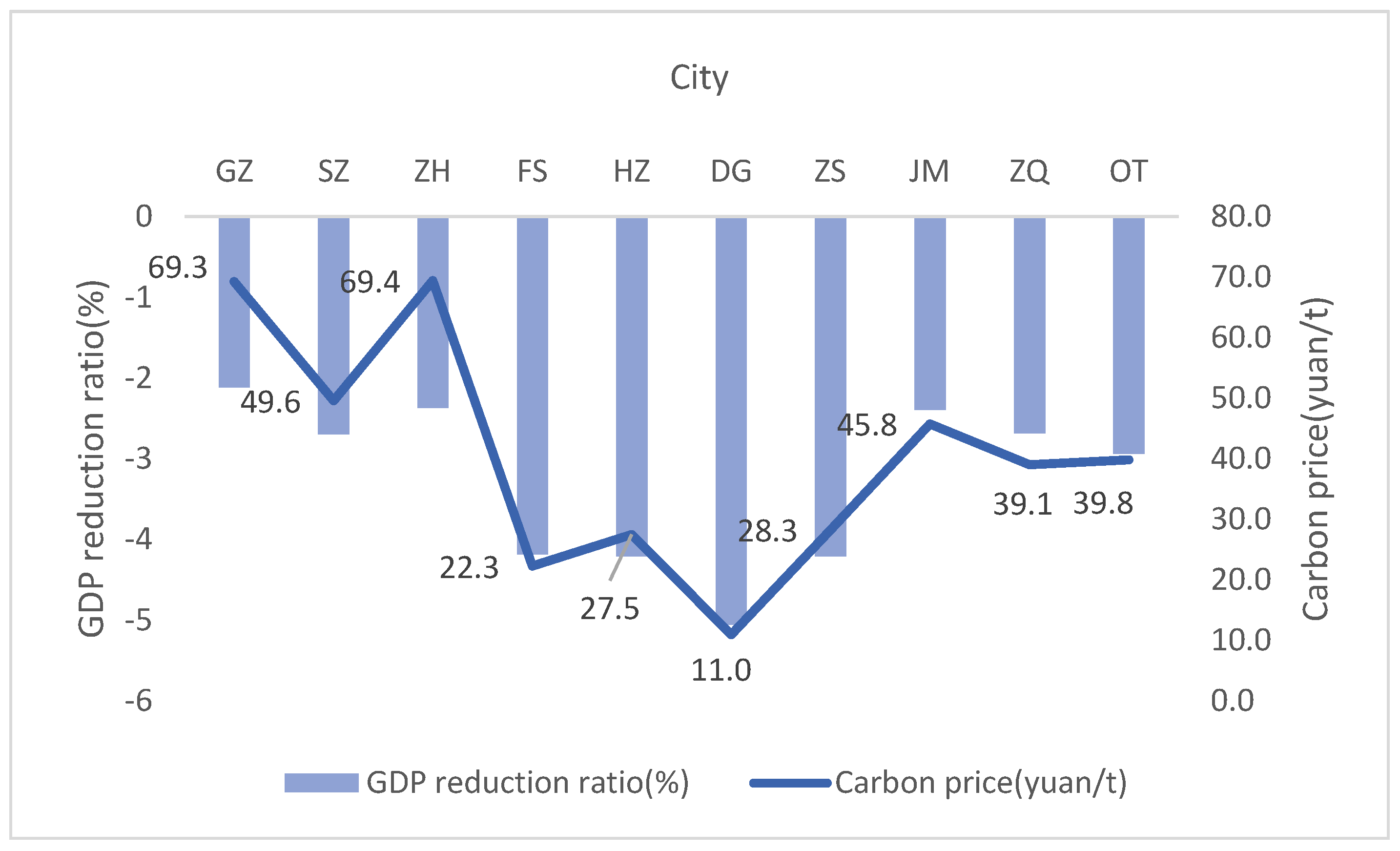
• Increasing the substitution elasticity of energy–labor and capital reduces the carbon price and the opportunity cost of carbon reduction. Carbon prices are also affected by macro-closure conditions. Under Keynesian closure conditions, carbon prices are negatively correlated with the degree of economic impact on cities, and those with greater impact are more sensitive to carbon prices with lower carbon prices at the same emissions reduction rate.
• The economic impacts of carbon emissions reduction on cities have similarities and differences. Under neoclassical conditions, owing to the influence of carbon prices, the production costs of most sectors increase, and demand decreases accordingly. Thus, the total social output value, GDP, import and export, government income, and household consumption of most cities decrease. A few cities (e.g., Dongguan and Jiangmen) enjoy GDP increases because carbon emissions reduction causes labor and capital to transfer to low-carbon industries, and those sectors play a role in supporting the main industries of the city. Thus, the overall GDP increases. Under Keynesian conditions, all industries are generally impacted, with carbon- and trade-intensive sectors being the most affected. No industry benefits from emissions reductions, but sectors with less trade are relatively less affected.

To ensure the achievement of emissions reduction targets and to minimize economic impacts, those impacts must be fully accounted for during carbon quota allocation.

The following suggestions are proposed from the combined perspectives of fairness and efficiency:

• The allocation of city-level carbon quotas should consider the current energy and industrial structural characteristics of cities, while considering the emissions reduction costs of each. Cities sensitive to carbon prices should not aim too high (e.g., Foshan).
• Moderate subsidies and support should be given to high-carbon energy industries, which are greatly affected during carbon emissions reduction, to ensure the stability and orderly optimization of their economic structures.
• For trade-oriented cities, because they are relatively sensitive to carbon prices, special attention should be paid to the low-carbon support and guidance of the leading trade industries (e.g., Shenzhen and Dongguan).

References

1. Kyoto Protocol to the United Nations Framework Convention on Climate Change. Available online: https://unfccc.int/process-and-meetings/the-kyoto-protocol/history-of-the-kyoto-protocol/text-of-the-kyoto-protocol (accessed on 24 July 2022).
2. Paris Agreement. Available online: https://unfccc.int/process-and-meetings/the-paris-agreement/the-paris-agreement (accessed on 24 July 2022).
3. EU Emissions Trading System (EU ETS). Available online: https://icapcarbonaction.com/en/ets/eu-emissions-trading-system-eu-ets (accessed on 24 July 2022).
4. He, X. Regional differences in China’s CO2 abatement cost. Energy Policy 2015, 80, 145–152. [Google Scholar] [CrossRef]
5. Jiang, J.; Xie, D.; Ye, B.; Shen, B.; Chen, Z. Research on China’s cap-and-trade carbon emission trading scheme: Overview and outlook. Appl. Energy 2016, 178, 902–917. [Google Scholar] [CrossRef]
6. Liu, J.-Y.; Feng, C. Marginal abatement costs of carbon dioxide emissions and its influencing factors: A global perspective. J. Clean. Prod. 2018, 170, 1433–1450. [Google Scholar] [CrossRef]
7. China’s Achievements in Implementing National Independent Contributions and New Goals and Measures. Available online: http://us.china-embassy.gov.cn/zt_1/ydqhbh/202111/P020211106160885316810.pdf (accessed on 24 July 2022). (In Chinese)
8. Outline of the 14th Five-Year Plan for National Economic and Social Development of Guangdong Province and the Long-term Goals for 2035. Available online: https://www.gd.gov.cn/zwgk/wjk/qbwj/yf/content/post_3268751.html (accessed on 24 July 2022). (In Chinese)
9. Zhou, J.-F.; Wu, D.; Chen, W. Cap and Trade Versus Carbon Tax: An Analysis Based on a CGE Model. Comput. Econ. 2021, 59, 853–885. [Google Scholar] [CrossRef]
10. Van den Bergh, K.; Delarue, E. Quantifying CO2 abatement costs in the power sector. Energy Policy 2015, 80, 88–97. [Google Scholar] [CrossRef]
11. Kong, L.; Hasanbeigi, A.; Price, L.; Liu, H. Energy conservation and CO2 mitigation potentials in the Chinese pulp and paper industry. Resour. Conserv. Recycl. 2017, 117, 74–84. [Google Scholar] [CrossRef]
12. Huang, Y.-H.; Wu, J.-H. Bottom-up analysis of energy efficiency improvement and CO2 emission reduction potentials in the cement industry for energy transition: An application of extended marginal abatement cost curves. J. Clean. Prod. 2021, 296, 126619. [Google Scholar] [CrossRef]
13. Wang, K.; Wei, Y.-M. China’s regional industrial energy efficiency and carbon emissions abatement costs. Appl. Energy 2014, 130, 617–631. [Google Scholar] [CrossRef]
14. Yang, L.; Tang, K.; Wang, Z.; An, H.; Fang, W. Regional eco-efficiency and pollutants’ marginal abatement costs in China: A parametric approach. J. Clean. Prod. 2017, 167, 619–629. [Google Scholar] [CrossRef]
15. Huang, S.K.; Kuo, L.; Chou, K.-L. The applicability of marginal abatement cost approach: A comprehensive review. J. Clean. Prod. 2016, 127, 59–71. [Google Scholar] [CrossRef]
16. Wang, P.; Dai, H.-c.; Ren, S.-y.; Zhao, D.-q.; Masui, T. Achieving Copenhagen target through carbon emission trading: Economic impacts assessment in Guangdong Province of China. Energy 2015, 79, 212–227. [Google Scholar] [CrossRef]
17. Wu, R.; Dai, H.; Geng, Y.; Xie, Y.; Masui, T.; Tian, X. Achieving China’s INDC through carbon cap-and-trade: Insights from Shanghai. Appl. Energy 2016, 184, 1114–1122. [Google Scholar] [CrossRef]
18. Cui, L.; Fan, Y.; Zhu, L.; Bi, Q. How will the emissions trading scheme save cost for achieving China’s 2020 carbon intensity reduction target? Appl. Energy 2014, 136, 1043–1052. [Google Scholar] [CrossRef]
19. Tang, B.-J.; Ji, C.-J.; Hu, Y.-J.; Tan, J.-X.; Wang, X.-Y. Optimal carbon allowance price in China’s carbon emission trading system: Perspective from the multi-sectoral marginal abatement cost. J. Clean. Prod. 2020, 253, 119945. [Google Scholar] [CrossRef]
20. Wu, J.; Fan, Y.; Timilsina, G.; Xia, Y.; Guo, R. Understanding the economic impact of interacting carbon pricing and renewable energy policy in China. Reg. Environ. Chang. 2020, 20, 74. [Google Scholar] [CrossRef]
21. Kim, E.; Kim, K. Impacts of regional development strategies on growth and equity of Korea: A multiregional CGE model. Ann. Reg. Sci. 2002, 36, 165–180. [Google Scholar] [CrossRef]
22. Development Prospects Group (DECPG). Linkage Technical Reference Document, Version 6.0; The World Bank: Washington, DC, USA, 2005. [Google Scholar]
23. Hertel, T.W. Global Trade Analysis: Modeling and Applications. Master’s Thesis, Cambridge University Press, Cambridge, UK, 1997. [Google Scholar]
24. Horridge, M.; Madden, J.; Witter, G. Using a highly disaggregated multiregional single-country model to analyze the impacts of the 2002-03 drought on Australia. J. Policy Model. 2005, 27, 285–308. [Google Scholar] [CrossRef]
25. Yuan, Y.-N.; Li, N.; Shi, M.-J. Construction of China’s multi regional CGE model and its application in carbon trading policy simulation. Math. Pract. Theory 2016, 46, 106–116. (In Chinese) [Google Scholar]
26. Pang, J.; Timilsina, G. How would an emissions trading scheme affect provincial economies in China: Insights from a computable general equilibrium model. Renew. Sustain. Energy Rev. 2021, 145, 111034. [Google Scholar] [CrossRef]
27. Hou, H.-P. Research on the Construction and Influencing Factors of High-Quality Development Evaluation Indicators in the Guangdong-Hong Kong-Macao Greater Bay Area. Master’s Thesis, Guangdong University of Foreign Studies, Guangzhou, China, 2020. (In Chinese). [Google Scholar]
28. The State Council’s Proposal on Printing and Distributing the 13th Five-Year Plan Notification of the Work Programme for the Control of Greenhouse Gas Emissions. Available online: http://www.gov.cn/zhengce/content/2016-11/04/content_5128619.htm (accessed on 24 July 2022). (In Chinese)
29. Bian, Y. The Guangdong-Hong Kong-Macao Greater Bay Area Can Take the Lead in Achieving carbon neutrality. China Open. J. 2021, 3, 105–112. (In Chinese) [Google Scholar] [CrossRef]
30. Progress, Challenge and Trend of Carbon Market in Guangdong. Available online: https://www.efchina.org/Reports-zh/report-lceg-20220427-zh (accessed on 24 July 2022). (In Chinese).
31. China—Guangdong Pilot ETS. Available online: https://icapcarbonaction.com/en/ets/china-guangdong-pilot-ets (accessed on 24 July 2022).
32. China—Shenzhen Pilot ETS. Available online: https://icapcarbonaction.com/en/ets/china-shenzhen-pilot-ets (accessed on 24 July 2022).
33. Liu, L.; Sun, X.; Chen, C.; Zhao, E. How will auctioning impact on the carbon emission abatement cost of electric power generation sector in China? Appl. Energy 2016, 168, 594–609. [Google Scholar] [CrossRef]
34. Schmidt, R.C.; Heitzig, J. Carbon leakage: Grandfathering as an incentive device to avert firm relocation. J. Environ. Econ. Manag. 2014, 67, 209–223. [Google Scholar] [CrossRef]
35. Yi, W.-J.; Zou, L.-L.; Guo, J.; Wang, K.; Wei, Y.-M. How can China reach its CO2 intensity reduction targets by 2020? A regional allocation based on equity and development. Energy Policy 2011, 39, 2407–2415. [Google Scholar] [CrossRef]
36. Zetterberg, L.; Wrake, M.; Sterner, T.; Fischer, C.; Burtraw, D. Short-run allocation of emissions allowances and long-term goals for climate policy. Ambio 2012, 41 (Suppl. S1), 23–32. [Google Scholar] [CrossRef]
37. Data Reading Bay Area: Analysis on the Proportion of Import and Export Trade in Guangdong-Hong Kong-Macao Greater Bay Area. Available online: https://www.sohu.com/a/361857235_120303032 (accessed on 24 July 2022). (In Chinese).
38. Analysis Report on the Statistical Indicator System for the Moderate and Diversified Development of Macao’s Economy in 2018. Available online: http://www.dsec.gov.mo/Statistic/General/SIED/2018.aspx?lang=zh-CN (accessed on 24 July 2022). (In Chinese)
39. Chen, W.; Zhou, J.-F.; Li, S.-Y.; Li, Y.-C. Effects of an Energy Tax (Carbon Tax) on Energy Saving and Emission Reduction in Guangdong Province-Based on a CGE Model. Sustainability 2017, 9, 681. [Google Scholar] [CrossRef]
40. Zhang, M.; Fan, J.; Zhou, Y.-H. Compilation and updating of input-output tables for multiple regions within a province: A case study of Jiangsu Province. Stat. Res. 2008, 7, 74–81. (In Chinese) [Google Scholar] [CrossRef]
41. Zhou, J.; Liu, L.; Chen, W.; Wu, D. Study on implied carbon transfer in Guangdong Hong Kong Macao Great Bay Area. In Research Report on Ecological Civilization and Low Carbon Development in Guangdong Province; Fu, J., Ed.; Sun Yat-sen University: Guangzhou, China, 2020; pp. 113–123. (In Chinese) [Google Scholar]
Figure 1. Production module.
Sustainability 14 10756 g001
Figure 2. Trade module.
Sustainability 14 10756 g002
Figure 3. Relationship between emissions reduction intensity and carbon prices.
Sustainability 14 10756 g003
Figure 4. Carbon intensity and price.
Sustainability 14 10756 g004
Figure 5. Impact of carbon emissions reduction (5%) on gross domestic product (GDP) and carbon price (Keynes closure).
Sustainability 14 10756 g005