3.1. Basic Facts
As seen in
Figure 2, the overall trend of housing prices in Shanghai through Lianjia Real Estate during the past ten years kept rising even under the shock of the epidemic, demonstrating that housing prices in Chinese megacities are extremely stable, especially among high-priced houses. The number of second-hand housing transactions, meanwhile, has generally increased. In 2016, this reached a historical peak of 59,037 houses. In 2018, it was 31,034 houses. In 2020, after the impact of COVID-19, the transaction volume of second-hand housing in Shanghai rapidly increased to 53,965 houses. Shanghai’s excellent epidemic-prevention performance in 2020 provided residents with confidence in choosing to settle in this city. In 2021, after the epidemic in China was generally under control, second-hand housing transaction volume fell to nearly 30,000 houses, which meant that the market heat had subsided.
In the following content, we set aside the years 2018 and 2021 for comparison. As researched, the COVID-19 pandemic began at the end of 2019 [
65], and 2020 was the worst year since then; numerous people got infectious and even died, unfortunately. Therefore, we chose the year 2018—the year before 2019, and the year 2021—the year after 2020, as samples of pre- and post- pandemic. For further research, we delete the top 1% and bottom 99% of samples using Stata, then drop duplicated residential quarters of all the samples. Therefore, the total number of observations was 5548 in 2018 and 6042 in 2021. The average housing price per meter in Shanghai was nearly RMB 52,000 (USD 8000) in 2018 and about RMB 63,000 (USD 10,000) in 2021, which means that housing prices rose up to 21 percent during the last three years, equal to the growth of the per capita disposable income of residents and the inflation rate over the same period in Shanghai (RMB 64,183 in 2018 and RMB 78,027 in 2021).
Explanatory variables also show varying degrees of change (see
Table 2). In 2018, the average living area of a house was nearly 75 square meters, while the number increased by 13 square meters in 2021, with the fact that unit prices rose sharply, altogether reflecting a further polarization of housing prices in megacities in China. In addition, the average deal days of the second-hand house were about 5 months in 2018, which quickly dropped to 3 months in 2021. Early in 2018, Shanghai’s second-hand house transactions mostly concentrated on the middle floor of the building, while the pattern changed to the low and high floors in 2021. The total floors of the building reached up to 10 floors in 2018 and nearly 11 floors in 2021. Most of Shanghai’s apartments faced south or east (the percentage was as high as 97% in 2018 and slightly decreased to 96% in 2021), owned no more than 2 rooms, were aged more than 20 years (20 in 2018 and 23 in 2021), and building type was slab-type or a combination of slab-type and tower-type. Distance to the nearest metro station was 1211 m in 2018 and decreased to 1183 m in 2021, and the distance to the nearest bus station was 176 m in 2018 and decreased to 167 m in 2021, altogether reflecting better transportation convenience. The distance to the nearest primary school was 544 m in 2018, increasing to 550 m in 2021.
3.2. Spatial Auto-Correlation
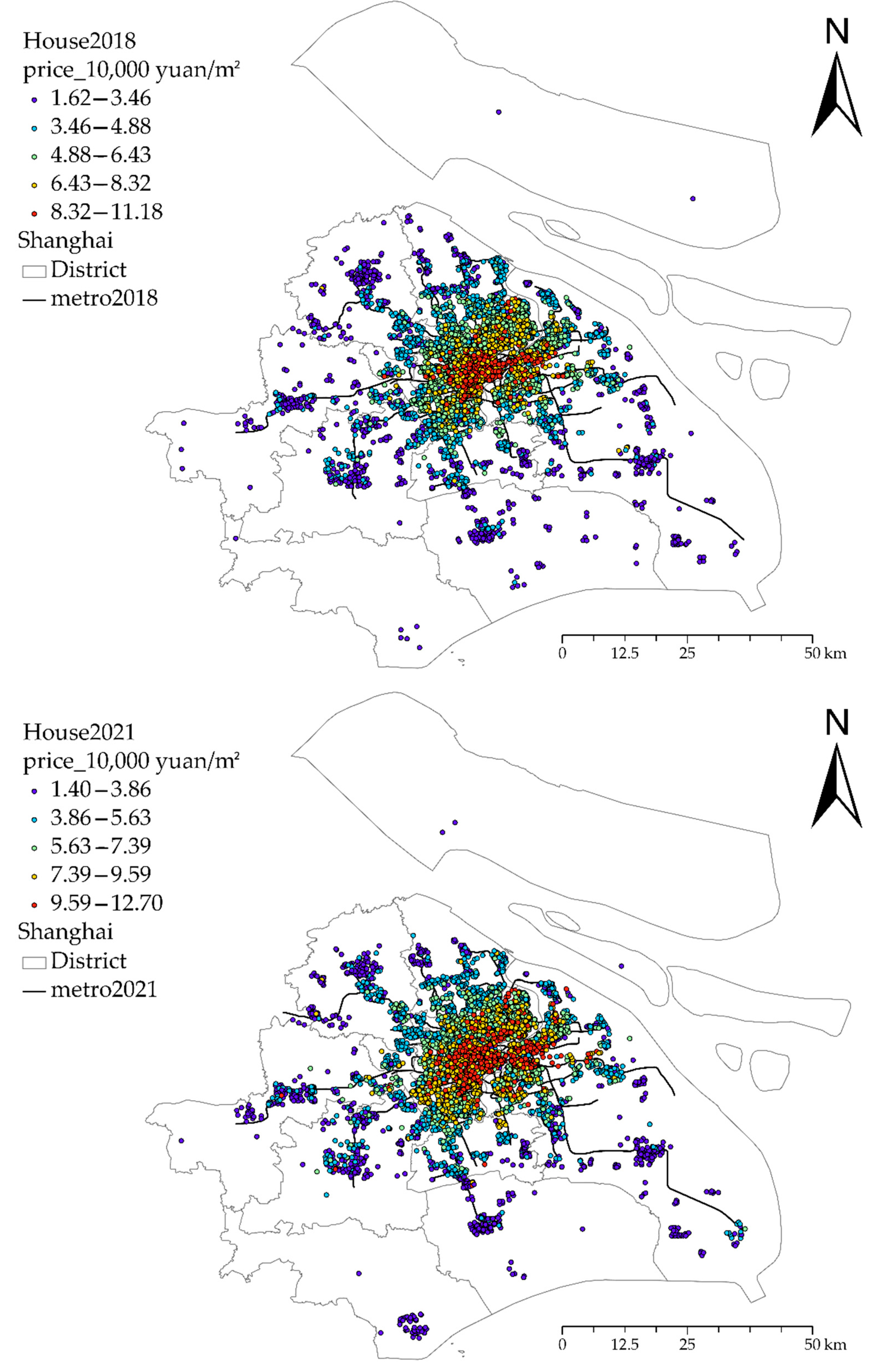
As seen in
Figure 3, second-hand housing prices in Shanghai are centered in the city’s downtown, spreading radially to the surrounding areas, with suburbs’ houses distributed mainly along the subway branch line, and remaining stable before and after the pandemic.
Specifically, in 2018, when classifying Shanghai’s housing prices into 5 groups using Jenks, the highest rank was more than RMB 83,000, with the highest price reaching up to RMB 112,000; while the lowest rank was less than RMB 35,000 with the lowest price as low as RMB 16,000. The gap between Shanghai’s most expensive house and the cheapest one reached as high as RMB 100,000 per square meter, more than the per capita disposable income of Shanghai residents throughout the year, revealing the huge spatial heterogeneity of Shanghai’s housing prices, prompting researchers to figure out its major influencing factors.
Similarly, Shanghai’s 5 grouped housing prices in 2021 also show significant polarization; the highest rank was more than RMB 96,000, with the highest price reaching up to RMB 127,000; while the lowest rank was less than RMB 39,000 with the lowest price as low as RMB 14,000. The gap between Shanghai’s most expensive house and the cheapest one further expanded. In addition, the higher level became more expensive compared to three years ago. In comparison, the lower level became cheaper, demonstrating that the polarization of housing prices in Shanghai further intensified.
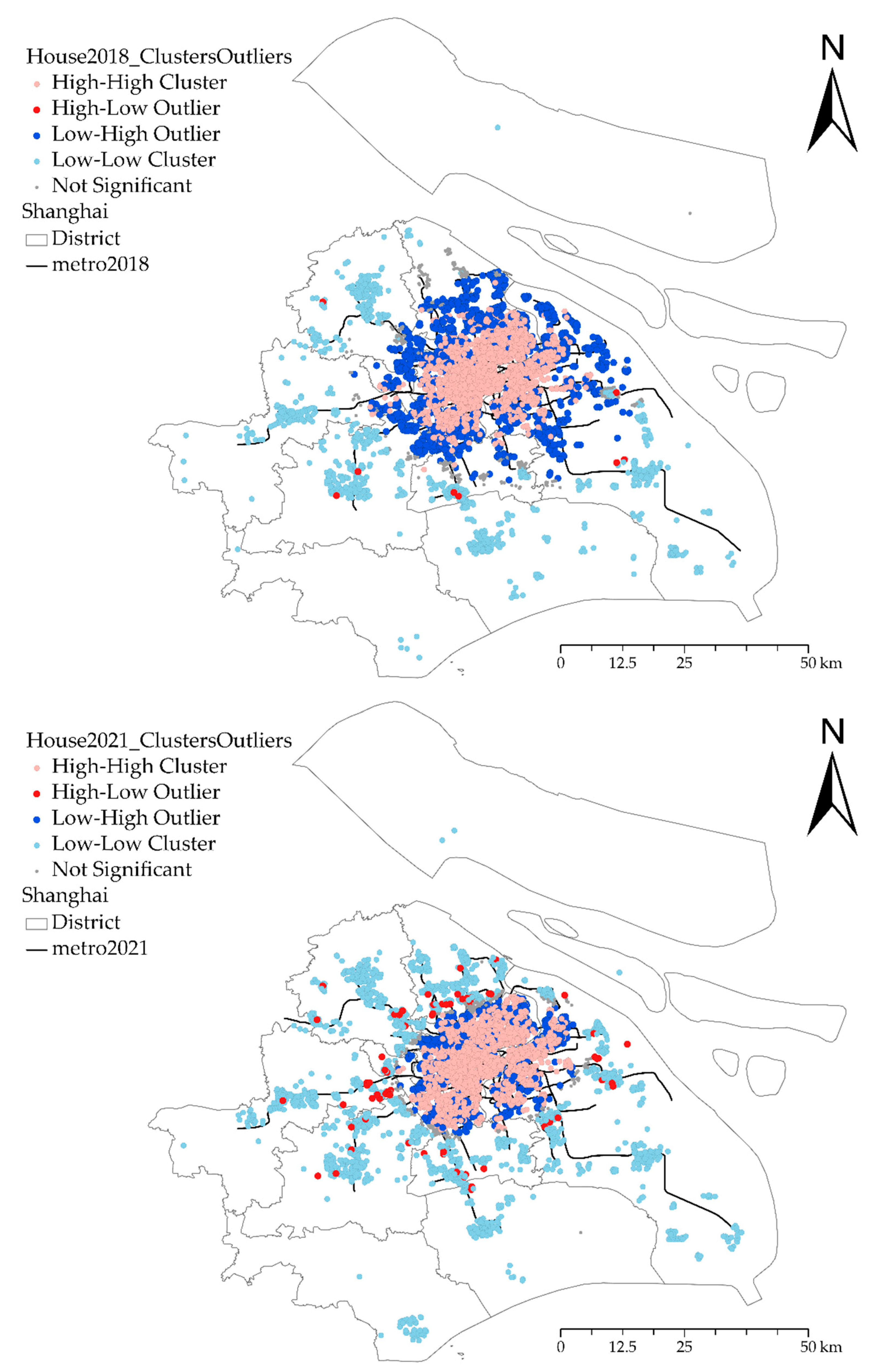
Table 3 shows global Moran’s I of the second-hand housing prices in Shanghai in 2018 and 2021. It is worth noting that the Moran’s I index is only appropriate for polygons; we clustered housing points into 215 streets/townships in Shanghai and calculated the results. The
p-value, which was almost zero for both years, indicates that both years’ housing prices were significantly positive at the level of 1%, which means these data are not a result of a random spatial process. The Moran’s I, which is 0.579 and 0.603 in the year 2018 and 2021, respectively, implies that expensive houses tend to cluster together, and so do the cheap ones. Moreover, the spatial agglomeration degree of Shanghai’s housing prices was higher after the pandemic. Therefore, the spatial autocorrelation may affect the subsequent analysis.
3.4. MGWR
Results of GWR and MGWR model indexes of Shanghai’s second-hand housing prices in 2018 and 2021 can be seen in
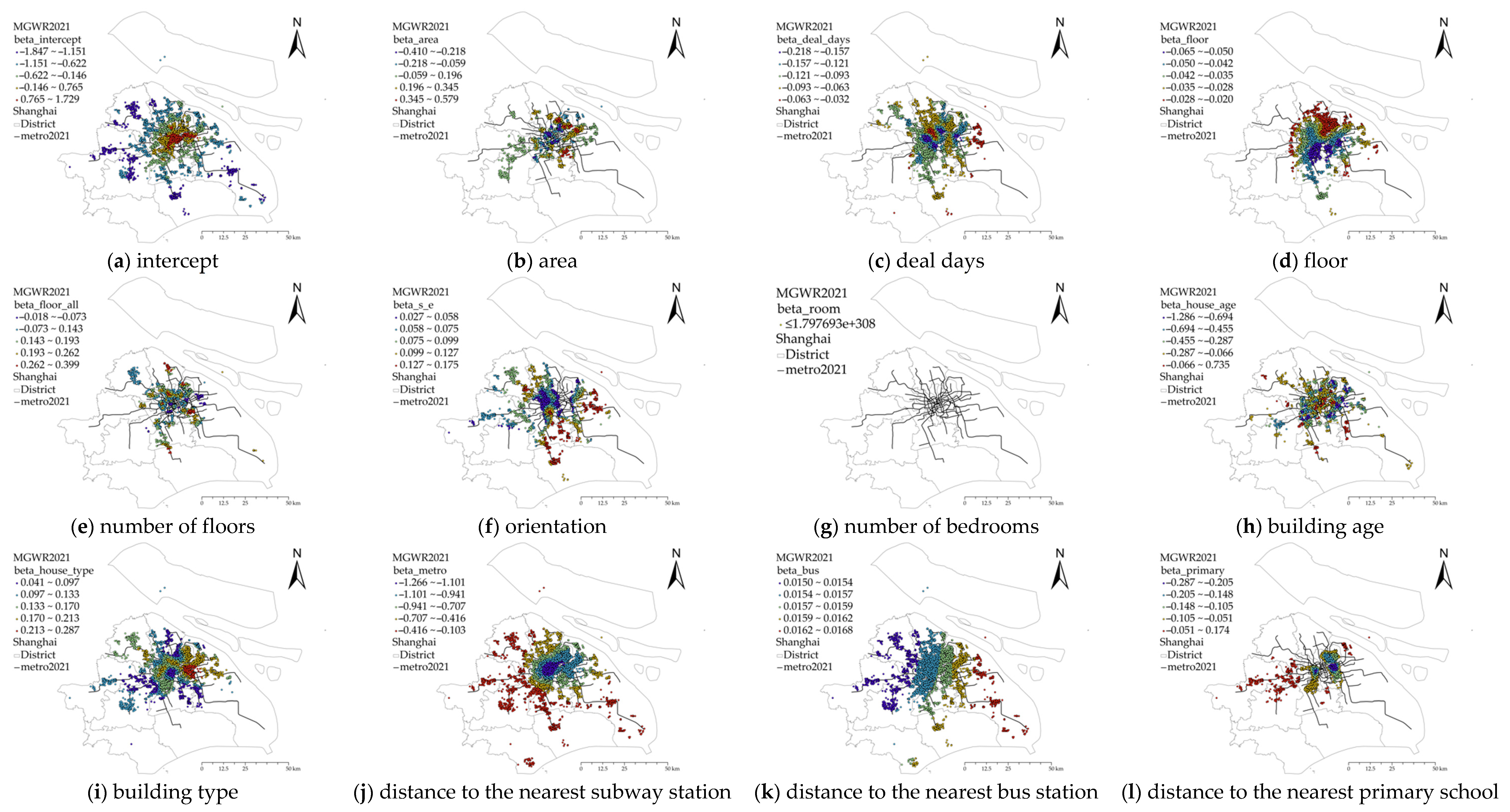
Table 4. Seemingly, in both years, the residual sum of squares of MGWR is smaller than that of classical GWR, the goodness-of-fit R2 of MGWR is significantly higher than that of classical GWR, and the AICc value is lower than that of classical GWR. Therefore, it can be concluded that the result of MGWR is better than that of classical GWR. On the other hand, from the overall regression coefficient, almost all the coefficients of MGWR were significant—only significant results were drawn on the map, as shown in
Figure 6 and
Figure 7. In contrast, most coefficients of classical GWR are not statistically significant (not shown due to space constraints), which is unreasonable, and implies that the classical GWR ignores the diversification of the scale of each variable, resulting in a lot of noise and bias in the regression coefficients, and finally leads to inconsistencies in the regression coefficients. Therefore, based on the analysis results of this case, it is found that the MGWR model is superior to the classical GWR model, even under the shock of the pandemic.
It can be seen from
Table 5 that MGWR can directly reflect the differential action scale of different variables. In contrast, the classical GWR can only reflect the average value of the action scale of each variable. The bandwidth of the classic GWR was 398 in 2018 and 285 in 2021, which was only 7.2% and 4.7% of the total sample size. By calculating MGWR, it was found that the scale of action of different variables varies greatly.
In 2018, the MGWR regression coefficients of 11 variables (namely constant term, area, transaction days, floor, number of floors, orientation, number of bedrooms, building age, building type, distance to the nearest subway station, and distance to the nearest bus station) were significant overall. However, the regression coefficient of distance to the nearest primary school was not significant. In 2021, the MGWR regression coefficients of 11 variables were also significant overall, except for the number of bedrooms.
The constant term represents the influence of different locations on house prices when other independent variables are determined. This paper controls traffic factors, so the constant term reflects the influence of other location factors such as school district and built environment on housing prices. The action scales were 44 in 2018 and 43 in 2021, accounting for 0.8% and 0.7% of the total sample size, which was much lower than the action scale of other variables, revealing that second-hand housing prices are very sensitive to the location in Shanghai.
In 2018, the role scale of the building age, living area, and building type were very small, accounting for less than 2.0% of the total sample size, indicating that those explanatory variables have large spatial heterogeneity. Action scales of the transaction days, number of bedrooms, and distance to the nearest bus station were relatively small, and the coefficient was relatively stable in space. However, effect scales of the floor, total floors, orientation, distance to the nearest subway station, and distance to the nearest primary school were pretty large, which belong to the global scale; that is, there was almost no spatial heterogeneity. Similarly, action scales of the explanatory variables in 2021 were also classified into 3 types: (1) very small: building age, living area, and total floors of the building; (2) relatively small: distance to the nearest primary school, building type, transaction days, orientation, distance to the nearest subway station, and floor of the house; (3) pretty large: number of bedrooms and distance to the nearest bus station.
The statistical description of each coefficient of MGWR is shown in
Table 6. The impact of the location reflected by the constant term on the housing price was positive inside the Middle Ring Road and negative outside the Middle Ring Road in 2018, while positive inside the Inner Ring Road and negative outside the Inner Ring Road in 2021, showing an obvious circle structure in both years and an obvious shrinking range of expensive apartments after the pandemic, as can be seen in
Figure 6a and
Figure 7a.
As stated above, the action scale of different explanatory factors varies. In the MGWR model, a small variable coefficient means strong spatial heterogeneity; that is to say, the influence of this variable on housing prices varies greatly in communities with different geographical locations, which is shown as a relatively scattered distribution in the images, namely in
Figure 6b,h,i and
Figure 7b,d,h. On the contrary, a large variable coefficient means the variable has little effect on the housing price of different geographic locations and is shown through a regular color distribution in the images, namely,
Figure 6d–f,j,l and
Figure 7g,k.
The living area factor significantly impacts housing prices: negative inside the Inner Ring Road and outside the Outer Ring Road, while positive between those two roads in 2018 (see
Figure 6b). The above phenomenon remained largely stable in 2021, with the Pudong district changing from negative to positive inside the Inner Ring Road area (see
Figure 7b). Since Shanghai was developed from the central urban area, the average residential area is relatively small downtown, whereas land supply in suburban areas is relatively sufficient; thus, the average residential area is relatively large [
2]. Negative effects inside the Inner Ring Road reflect that due to the large area, high unit price, and the high total price, the demand decreases, and then the unit price decreases. On the other hand, negative effects outside the Outer Ring Road demonstrate that location advantage disappears as the living area increases, and unit prices need to decrease to appeal to consumers. Moreover, positive impacts between the Inner Ring Road and outside the Outer Ring Road reveal that those areas are most suitable for dwellers to live and work, contributing to the rise of unit prices as the living area increases.
The transaction days have a significant negative impact, meaning that the higher the unit housing price, the shorter the transaction days. In 2018, transaction days’ impact was only significant inside the Outer Ring Road, and the absolute value of the coefficient was especially smaller along the Huangpu River. Nonetheless, the overall difference was small (see
Figure 6c). In 2021, the absolute value of the coefficient rose sharply compared to that of 3 years ago (see
Figure 7c). This shows obvious differences spatially, and older residential areas in the city have more serious price cuts.
The floor of the house is negatively connected to the housing price (see
Figure 6d and
Figure 7d). The floor factor is a dummy variable, where a bigger number means a higher floor, and less than 40% of houses are equipped with an elevator. It is reasonable that the higher the floor is, the lower the unit price is. Regarding spatial heterogeneity, negative impacts were deeper in the north-west region and lighter in the south-east area in 2018, whereas deeper in the south-west region and lighter in the south-east area in 2021. On the whole, negative affection was reinforced after the pandemic.
Overall, the number of floors of the building was positively connected with the housing price; the higher the building is, the higher the unit housing price is (see
Figure 6e and
Figure 7e). A taller building means a higher probability of owning an elevator, thus making the positive relationship between the house’s total floor and its housing price. In 2018, all the sample’s coefficients were positive and varied little; in 2021, the significant range shrunk greatly, and few residential area coefficients turned negative.
The house orientation also positively affects the unit price of the house. As China is located in the northern hemisphere, a house facing south or east enjoys better lighting and ventilation, which makes it more comfortable to live in. The better the house orientation (facing south or east), the higher the unit price, and the influence of this factor decreases from south-east to north-west, as shown in
Figure 6f and
Figure 7f. The house orientation coefficient’s mean value was 0.028 in 2018 and 0.059 in 2021, meaning houses facing west or north were RMB 28/59 lower than those facing east or south (see
Table 6).
The number of bedrooms had a significant and negative impact on unit housing prices in 2018 but was not significant in 2021 (see
Figure 6g and
Figure 7g). In 2018, taking the downtown area as the core, the number of bedrooms had the greatest negative impact on the unit price, which spread outward in a circle with a gradually decaying effect. As mentioned above, housing prices in Shanghai are roughly distributed in a single-center pattern, with the highest housing prices in urban areas, which continue to decrease in circles. Therefore, high land prices in urban areas make the unit price of houses with fewer bedrooms and relatively smaller areas higher.
The influence of building age on the unit price was significantly negative in both years (see
Figure 6h and
Figure 7h). The building age coefficients’ mean value was −0.182 in 2018 and −0.204 in 2021, which means that for every 1-year increase in building age, the unit price of second-hand housing decreased RMB 182/204, reflecting that the negative impact of building age on housing prices is not different in different places, and its impact strength is weak (see
Table 6).
Building type is also a dummy variable; most houses in Shanghai are a combination of slab-type and tower-type. Compared to the slab-type building, the unit house price of the combination type is higher globally. At the same time, spatial heterogeneity was not significant in 2018 and was notably high in the Pudong district inside the Inner Ring Road area in 2021 (see
Figure 6i and
Figure 7i).
The distance to the nearest subway station negatively affected the house price, while the distance to the nearest bus station positively affected the house price in both years. The farther the distance to the nearest bus station, the higher the housing price, which means that for Shanghai, where the transportation network covers a wider area, the negative externalities (such as crowding and noise) generated by the bus station have exceeded the positive externalities (such as transportation convenience), which is consistent with previous similar research [
44,
66]. Accordingly, the above results demonstrate that the metro serves as Shanghai’s most important transport vehicle [
67]. In 2018, the distance to the nearest primary school showed no significant influence on the house price, while in 2021, the distance to the nearest primary school negatively affected the house price inside the Outer Ring Road while positively affecting the house price outside the Outer Ring Road, which reflects that families living near downtown care more about children’s education convenience (see
Figure 6j–l and
Figure 7j–l).


