Abstract
Air traffic complexity, an essential attribute of air traffic situation, is the main driving force of workload for air-traffic controllers and is the key to achieving refined air traffic control. The existing air traffic complexity studies are based on static network, ignoring the dynamic evolution of between-aircraft proximity relations. Research on such evolution course and propagation characteristics will help to comprehensively explore the mechanisms of complexity formation. Herein, an air traffic complexity propagation research method based on temporal networking and disease propagation modeling is proposed. First, a temporal network is built with aircraft as nodes and between-aircraft proximity relations as edges. Second, the disease propagation model is introduced to simulate the evolution course of between-aircraft proximity relations, and the propagation model is solved using Runge–Kutta algorithm and particle swarm optimization. Third, based on the solved results of the propagation model, the aircraft are divided into three groups with high, medium, and low propagation capability, respectively. Finally, the effects of different factors on the propagation course are analyzed using multivariate linear regression. Real data validation shows the propagation of high-propagation capability aircraft is significantly affected by duration, and the temporal-correlation coefficient. The propagation of medium-propagation capability aircraft is significantly affected by duration and the clustering degree. By adjusting the influencing factors, the air traffic complexity propagation process can be effectively controlled.
1. Introduction
Air traffic management is responsible for ensuring the safety and efficiency of air transport and is a major component of air transport management. With the increasing demand for air traffic within limited airspace resources, the management of air traffic became a major limitation of air transport management. To improve the capabilities of air traffic management, researchers have introduced the concept of air traffic complexity to improve the efficiency of air traffic. Based on complexity assessment and control, aircraft trajectories are more accurate, which helps to improve the capability of air traffic management. Therefore, understanding and controlling air traffic complexity becomes crucial for sustainability in air transport management. The main topics of air traffic complexity evaluation include traffic density [1,2], dynamic density [3,4], traffic flow disturbance [5,6], and intrinsicity [7,8,9]. In research on intrinsicity, a complexity model is built according to between-aircraft proximity relations, which is closest to the real microenvironment faced by air-traffic controllers in their works. Hence, profound research on intrinsicity can help largely reduce the control load.
The complex network theory is introduced to aviation research to greater systematically study the internal intricate relations of aviation. Though the history of complex network modeling is very short in the aerospace field [10,11], its systematic views are inspirations for air traffic management [12,13]. Air Safety Committee of Eurocontrol proposed a complexity index in 2006 and thus was the first to comprehensively describe the between-aircraft interactive relations [14]. The Committee divided the airspace into several cubic squares, and thought that the aircraft falling into the same square at the same time will interact. Wang introduced the complex network theory into air traffic situation modeling and thought air traffic situation complexity was basically the temporal and spatial dynamic associations among different components of air traffic situation [15]. They probed into the scientific problem of small-scale aggregation of aircrafts and proposed the concept and division algorithm of aircraft groups [15]. While the research targets were gradually expanded from single sectors to multiple sectors, the models were continuously improved. So far, multilayer multilevel network models and dynamic weighting network models have been built [16]. The complex network theory can macroscopically reveal the sum of all between-aircraft microscopic relationships in an airspace. However, the existing network models are all based on static networks, which are essentially the instantaneous complex states at a series of scattered time periods, but the knowledge of complexity evolution is still deficient.
Research of complex network dynamics such as disease and rumor propagation, node or edge fault propagation, and online random walking and searching, is fundamentally aimed to explore the evolution of a certain event in a network. The temporal network is one key part of network dynamics research. With the addition of the time dimension, more valuable information that cannot be acquired from static networks can be obtained. The types, models, topological structure measuring methods, and propagation dynamics research methods of temporal networks were already summarized [17,18]. So far, the main application of complex network dynamics into civil aviation systems is the delay propagation. Machine learning methods such as neural networks and random forests have been used to predict air traffic delays with good results, but the mechanism of delays cannot be obtained. Therefore, a disease propagation model was introduced [19,20]. Given the worldwide aircraft-borne propagation of infective diseases, Balcan modeled and predicted the infective disease propagation patterns using air traffic data, and made successful achievements [21,22]. Later, many analyses targeting at delay propagation gradually opened new perspectives to uncover the essence of the delay. However, some studies ignore the time effectiveness of networks [23,24,25,26,27] and fail to determine which factors a delay is caused by [28]. Then, dynamics research was already conducted from the perspective of temporal networks [29,30].
To date, there has been no research related to the propagation of air traffic complexity. Previous research focused on sector-level air traffic complexity assessment and prediction but did not consider the dynamic complexity impact of one aircraft on other aircraft from a microscopic perspective. This will not meet the trend of air traffic development, that is, accurate aircraft trajectories (4D trajectories). Therefore, from the perspective of the aircraft, this paper evaluates the dynamic impact of a given aircraft to minimize the impact on other aircrafts as much as possible. Effective modeling of complexity propagation can characterize the propagation mechanism of complexity, and by analyzing the influencing factors of propagation, air traffic complexity can be fundamentally controlled, and the workload of air traffic controllers can be reduced. To solve this problem, in this paper, a propagation model based on a temporal network is established. Specifically, the contributions of this paper are as follows: first, this paper defines the air traffic complexity propagation behavior, and proposes an air traffic complexity propagation model based on temporal networks; second, a numerical solution method of the propagation model based on Runge–Kutta and particle swarm optimization is proposed to reduce errors; then, the influencing factors of the propagation model are quantified to obtain the control strategy of the propagation process.
The organization structure of this paper is as follows: Section 2 describes the definition of propagation behavior in air traffic and the propagation modeling algorithm. Section 3 selects the influencing factors of the propagation model from the perspective of air traffic controller’s actual operation and complex network, and provides a quantitative method. Section 4 details the numerical calculation of the differential equations of the propagation model. In Section 5, the performance of the proposed method is verified by numerical simulations. Relevant work is summarized in Section 6.
2. Propagation Models
Recently, many studies demonstrated that the time effectiveness of interactive behaviors will remarkably affect networks. The existing propagation models can be divided into synchronous and asynchronous interactions. In synchronous interactions, the between-node interactions occur and end both instantaneously, and the between-node edges are temporary and instantaneous. This pattern consists of a triplet series, which means the duration time of between-node interactive behaviors is ignored. The triplet indicates the events between nodes and at time . In asynchronous interactions, the events will persist for a certain time, so the information propagation between node pairs is delayed to some extent. For instance, viruses are transmitted via E-mails on the Internet, and the time of delivering viruses from the sender is always earlier than the time of activating the virus by the receiver. The asynchronous interaction pattern can be expressed by a quadruple series. The quadruple represents the events between nodes and , and the starting time is , and the duration time is . When node delivers a message to node , node can decide whether to accept this message or not at time t .
In the susceptible-infected-susceptible (SIS) model, a classic disease propagation model, nodes exist in two states: the susceptible status and the infected status. The nodes under the susceptible state may be converted, after a certain between-node interactive behavior, at a certain infection rate to the infected state. In the meantime, the nodes under the infected status are recovered at a certain rate to the susceptible state. The whole dynamic process is a recycle where the susceptible nodes transit to infected nodes, which then transit to susceptible nodes again.
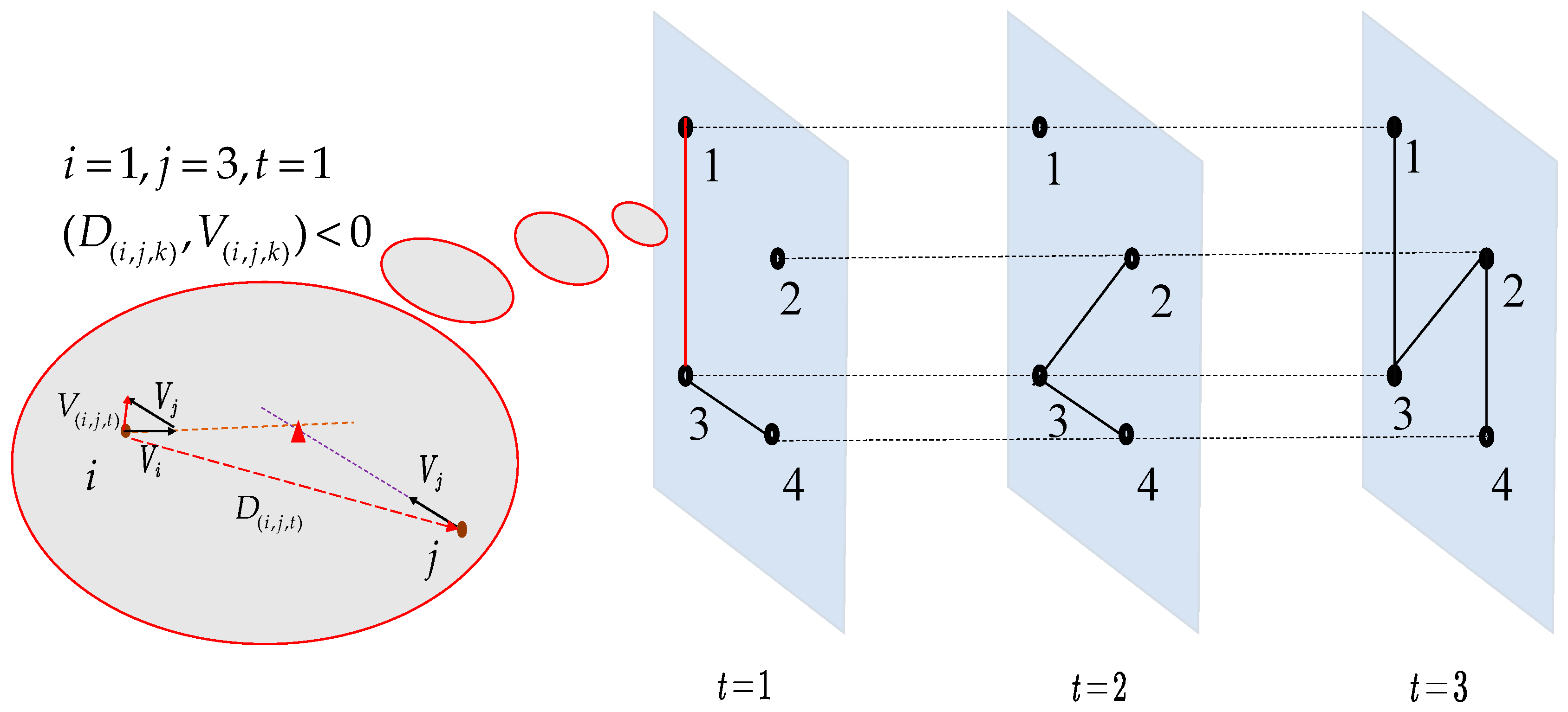
Given the real characteristics of air traffic situation temporal networks, we adopted the synchronous interaction mode. A simple air traffic situation temporal network is illustrated in Figure 1. There are three time layers in this temporal network. In each time layer, nodes are aircraft, and edges are between-aircraft proximity relations. Compared with the static network, we can mine more information in the temporal network. For instance, the degree of node three is two in the static network at different time layers; therefore, we cannot detect the change of the connection edge. However, we can easily find this information in a temporal network, which is important for studying the evolution of air traffic complexity.
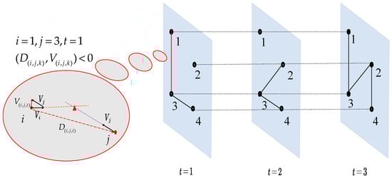
Figure 1.
Diagram of air traffic situation temporal network. Node: aircraft; Edge: between-aircraft proximity relation.
2.1. Definition of Air Traffic Complexity Propagation Behavior
In an air traffic situation temporal network, the nodes are aircraft. Let the relative velocity and distance of an aircraft pair be and at time t. After continued movement at the current velocity for 5 min, if a proximity relation exists at time k , namely the inner product , then the edges in the temporal network are connected in network layer t (Figure 1), and the time interval between network layers is 1 min. With aircraft as the propagation source, the aircraft pair get closer. Then, aircraft gradually influences the movement of aircraft j, so the air traffic complexity of aircraft j is gradually increased. Then, aircraft j is thought to be infected by the interaction from the proximity relation: namely aircraft j transits from a non-source aircraft to a source aircraft. The infection relations in the air traffic complexity propagation model are exactly established on the basis of between-aircraft proximity relations.
Similarly, the source aircraft will transit to a non-source aircraft through a certain behavior. Suppose aircraft j transits to a source aircraft at time t under the infection by aircraft . As time goes, such infection relation is gradually weakened and is related to the current and previous states of the two aircraft. Namely, the state of aircraft j at time is affected by the coupling relations of aircraft at different time points of the period . Reportedly, the coupling relation is gradually weakened with the increasing number of time layers [31]. The coupling degree between nodes at different time layers can be better described using the time attenuation factor. The different interlayer relations are decided by the selection of the attenuation factor and the features of the time-effective network. Given the high heterogeneity of between-node interactive behaviors in the air traffic situation time-effective network, we introduce an attenuation factor:
where is the time interval between two time layers and ; is the attenuation factor adjustment coefficient.
In the air traffic complexity propagation model, let ; when the interval is five, the attenuation factor is . When the interval is larger than five, the value of can be ignored, namely the interlayer effect can be ignored. Thus, when the recovery relation of the propagation model is studied, the interval between propagation influence time layers is set to be five. Namely, aircraft j is converted from a non-source aircraft to a source aircraft at time t. If aircraft j is not newly infected at time period , then aircraft j is recovered and its state transits from a source aircraft to a non-source aircraft.
2.2. Modeling of Air Traffic Complexity Propagation
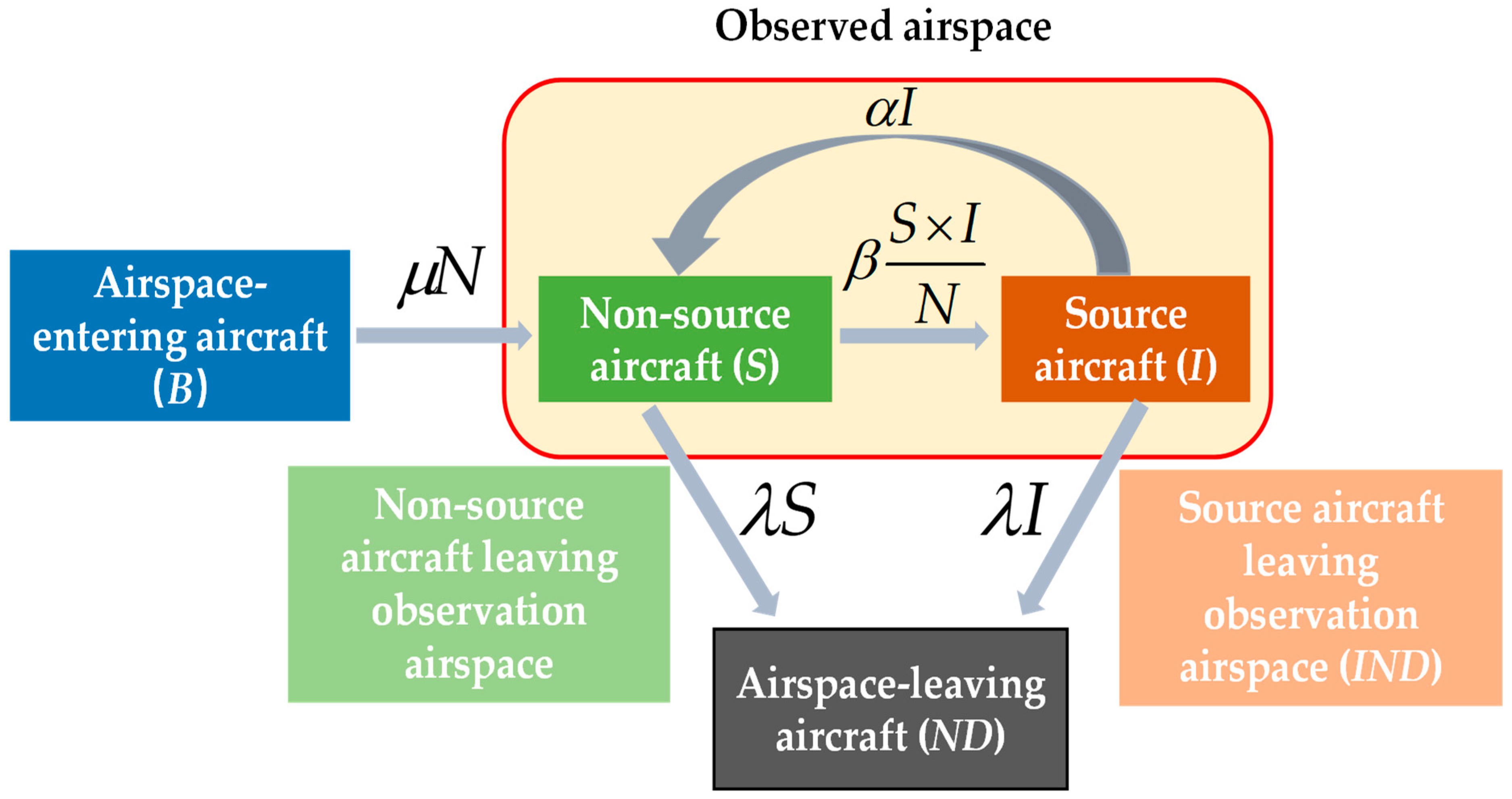
To better resemble the real features of air traffic operation, we add two new states (entering airspace, leaving airspace) into the air traffic complexity propagation model, in addition to the classic non-source state and the source state in the SIS model. We set two node states, including the active state and the inactive state. If any aircraft node appears within the observed airspace at time t, it is marked as the active state; otherwise, it is marked as the inactive state.
Airspace-entering aircraft (B): In a given airspace, if an aircraft node is inactive at time t and active at time , then node is considered as an entering aircraft at time ; namely, aircraft enters the observed airspace at time .
Airspace-leaving aircraft (ND): In the given airspace, if an aircraft node is active at time t and inactive at time , then node is considered as a leaving aircraft at time ; namely, aircraft leaves the observed airspace at time .
Source aircraft (I): any aircraft at the active state and being a propagation source.
Non-source aircraft (S): all aircraft at the active state that are not the propagation source.
The air traffic complexity propagation model is illustrated in Figure 2, where are the entrance rate, recovery rate, infection rate, and leaving rate, respectively. The differential equation of the propagation model is:

Figure 2.
Diagram of the air traffic complexity propagation model.
3. Influence Factors of the Propagation Model
In traditional disease propagation models, the features of the propagation source, susceptible population, and propagation route decide the infection rate and recovery rate. For instance, a person infected by a certain disease enjoys frequent social activities and closely and chronically contacts with others. In the community where he lives it is highly populated, and he contacts frequently with those living here, which all accelerates disease propagation. The case in the air traffic situation temporal network is the same; individual aircraft, airspace, and evolution all decide the features of the propagation. Here, we studied the effects of three factors on the propagation process, including individual features of nodes (propagation source), global features of the airspace (susceptible population), and node and network evolution features (propagation route). The individual features of nodes include the relative velocity of aircraft nodes, and the duration in a given airspace. The global features of the airspace include the clustering situations (clustering degree) of all aircraft, corresponding to the adjustment of speed, time, and safety interval in actual control operations. The node and network evolution features are the temporal-correlation coefficients of nodes and the network. Generally, if the velocity of an aircraft deviates more from the average velocity of all aircraft in the airspace and lasts for longer time, the clustering degree of aircraft within a certain space is higher, the interactions between nodes and between networks are more frequent, then the between-aircraft complexity propagation is faster. To scientifically analyze all influence factors, we first quantify the individual features of nodes, the global features of the airspace, and the node and network evolution features. Then, the relations of these features with infection rate and recovery rate are expressed using multiple linear regression. Finally, the effects of features on propagation are analyzed from the aspects of infection rate and recovery rate.
3.1. Relative Velocity and Duration
Numerous real data demonstrate that the aircraft moving velocities in an airspace obey the normal distribution, owing to the effects of aircraft performance, airway, and control. With two aircraft at the same flying height and direction as an example, if the two aircraft fly at similar velocities, the proximity relation between them can be ignored. If the front aircraft has a smaller velocity and the back aircraft has a larger velocity, they will form a proximity relation. In practical air traffic control, the controller assigns the entering aircraft with a certain interval. If all aircraft in the airspace fly at closer velocities, the number of potential proximity relations is smaller. Let the average velocity of all aircraft in the airspace be ; then the relative velocity of aircraft is , where is the velocity of aircraft . When is >0, the velocity of aircraft is larger than the average velocity of all aircraft in the airspace. A larger absolute value of the relative velocity means the aircraft deviates more from the average velocity.
The time period from when aircraft enters the observed airspace to when it leaves the airspace is called its duration and is marked as .
3.2. Clustering Degree
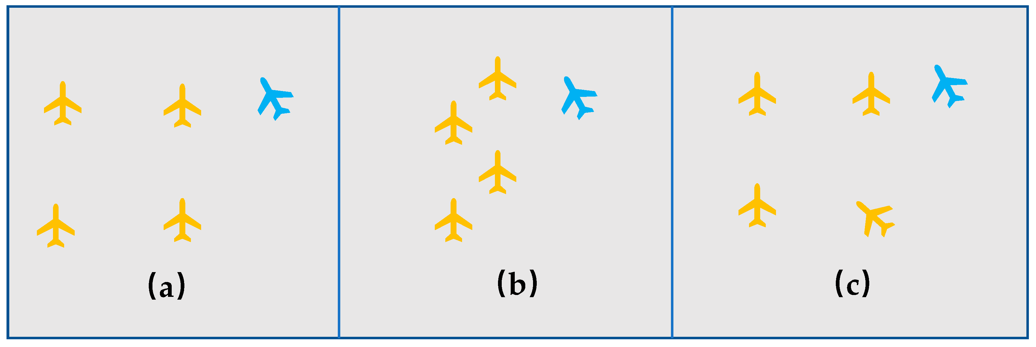
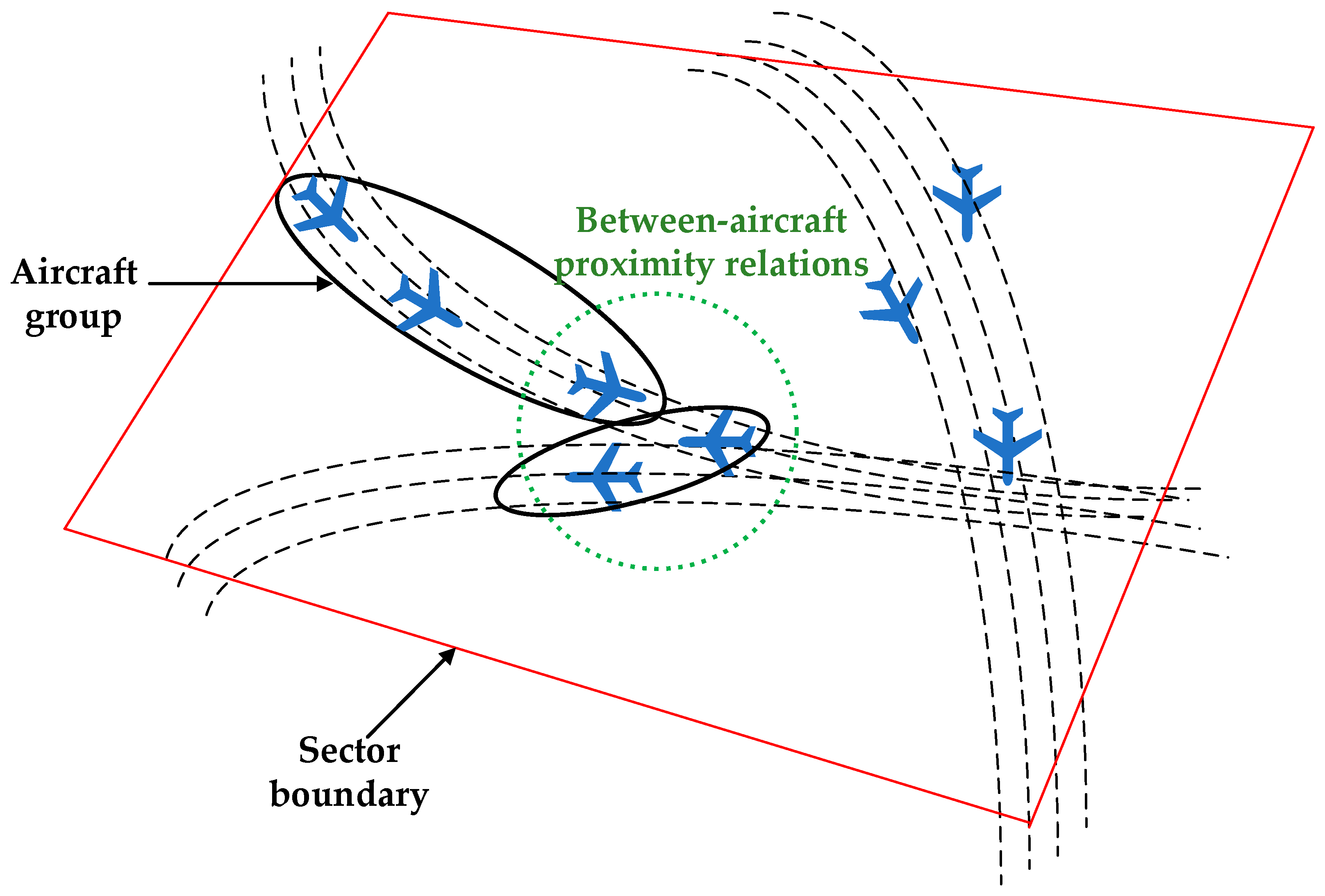
Figure 3 shows three simple air traffic scenarios, where yellow and blue represent non-source and source aircraft, respectively. The non-source aircraft are located closer in scenario b than in scenario a. If the velocities and directions of all aircraft are both the same between the two scenarios, after the source aircraft and non-source aircraft in scenario b constitute interactions, the behaviors will be rapidly transmitted to the four non-source aircraft. Moreover, the clustering degrees of aircraft are the same between scenarios a and c. In scenario c, the velocity of one aircraft obviously deviates, so the interactions between source-aircraft can only be transmitted to three aircraft. Thus, to portray the environment of the aircraft more scientifically, we classify the aircraft with close positions and velocities into the same group (Figure 4). Such disease propagation in an aircraft cluster is similar to the propagation among families of a community, where the individuals of a family have similar behavioral features, and the features among different families are much diverse. Generally, when a member in a certain family is infected, his family members are more susceptible to infection than other people in the community. Thus, such community and family relations can be measured using the clustering degree. Let the clustering degree of the aircrafts in the whole airspace be the sum of clustering degrees in different aircraft clusters. A higher clustering degree of aircraft in an airspace means the complexity propagation ability is stronger.
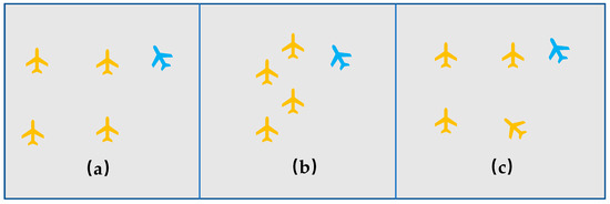
Figure 3.
Simple Air Traffic Scenario. (a): four non-source aircraft with the same velocity; (b): four non-source aircraft with the same velocity and closer distance; (c): Three of the four non-source aircraft with the same velocity; Blue aircraft: source aircraft; Yellow aircraft: non-source aircraft.
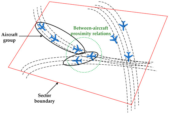
Figure 4.
Schematic diagram of aircraft group. Red square: sector boundary; Black circle: aircraft group; Green circle: between-aircraft proximity relations; Black dotted line: route.
3.2.1. Aircraft Group Division
One classic algorithm of aircraft group division is K-means clustering, which clusters the positional information of aircraft according to the given number of groups. In the resulting aircraft groups, the between-aircraft positions in the same group are relatively close, and the between-aircraft positions between groups are relatively far. In the air traffic complexity propagation model, because of requirements of the propagation mode, the aircraft at close position and different velocities shall be assigned to different groups. Given the high heterogeneity of movement among aircraft in the airspace, the number of aircraft groups cannot be preset, and the K-means algorithm has some limitations. Thus, the hierarchical clustering algorithm is used here. The aircraft groups at different directions and close positions can be automatically divided by adding a direction factor and improving the selection of clustering results.
- Preprocessing of trajectory data
The real radar data are a series of consecutive dots at the same time interval, marked as , where is the positional information of an aircraft at time , ; are the horizontal, vertical, and height coordinates of the aircraft at time , respectively. After processing of the radar data, we can determine the horizontal, vertical, and height coordinates, velocity, and direction of the aircraft at a certain time point.
In a certain sector, aircraft can be regarded as mass points. The set of aircraft positions and velocities of a sector are expressed as the following matrix:
where is the information of aircraft ; are the horizontal, vertical, and height coordinates of aircraft ; are the velocity components at three axes of aircraft .
As the units of position and velocity are different among aircraft, the data shall be normalized (Z-Score):
where is the mean of , is the standard deviation of .
- 2.
- Clustering algorithm
The steps of the hierarchical clustering algorithm are as follows:
Step1: Define the initial aircraft group, let each aircraft in a sector be an initial aircraft group, and let be the aircraft group .
Step2: Calculate distance—with the Euclidean distance, calculate the distances between any pair of aircraft and in the sector:
Record the calculated results in a distance matrix .
Step3: Combine the aircraft groups; find the minimum element in the distance matrix :
Combine and into a new aircraft group: , namely.
Step4: Recalculate the minimum distance between groups. Calculate the distance between the new aircraft group and other aircraft groups in the set:
Update the distance matrix by using the calculated results, and combine the rows and columns that involve and into new rows and columns. As for , the distances of the new and other aircraft groups are updated, whereas other rows and columns are unchanged. Record the new distance matrix as .
Step5 Circulate the computation. Repeat steps (3) and (4) with until reaching a new matrix. In this way, all aircraft groups are combined into only one group.
Step6 Draw a spectrum. Plot a clustering spectrum according to the results in the above five steps.
Step7 Determine the result of clustering. Based on the calculated distortion degrees, select the optimal number of responsive groups, and determine the final clustering result.
- 3.
- Determination of clustering result.
The elbow method is used to analyze the spectra obtained from the clustering algorithm. The distortion degree is defined as the sum of squares of positional distance in the center-of-mass in an aircraft group from other aircraft. Suppose aircraft are assigned to groups (, namely at least one group has two aircraft). Then let be aircraft group , and the center-of-mass of this group is . Then, the distortion degree of group is .
The total distortion degree of all aircraft groups is considered as the clustering coefficient :
Then the total clustering coefficient of aircraft is ().
Let be the distortion trend of clustering results . If , then the optimal number of groups is .
3.2.2. Computation of Clustering Degree
The clustering degree of an aircraft group reflects the propagation features among aircraft that have similar local features in propagation behaviors. The clustering degree is low when a group has only a few aircrafts. The clustering degree is intensified with the increase in the number of aircraft. In aircraft groups with the same number of aircraft, the clustering degree is higher when the aircraft are positioned closer. The clustering degree within an aircraft group, , is calculated as:
where is the distance from aircraft in the group to the center-of-mass of the group; is the total number of aircraft in the group.
The position of aircraft is :
The center-of-mass of aircraft in the group is :
where is the number of aircraft in the group that contains aircraft .
Thus, the clustering degree of the group is defined as:
where is the weight regulatory factor; is the total number of aircraft in the group that contains aircraft .
When an aircraft is far away from the center-of-mass, a larger means the resulting value of the clustering degree is lower. When an aircraft is closer to the center-of-mass, a smaller means the clustering degree is larger.
Here, we chose , so the within-group clustering degree is:
The clustering degree of all aircraft in the airspace is:
where is the number of aircraft groups; is the within-group clustering degree of group .
3.3. Nodes and Network Evolution Features
In an air traffic situation time-effective network, two aircraft in a proximity relation have edges, and when the edges change, the propagation behaviors also change. Thus, the propagation behaviors at nodes can be judged according to the changes in the edges at the nodes at different time points in the time-effective network.
The evolution of edges in the time-effective network can be expressed as the network temporal-correlation coefficient :
where is the number of nodes in the network; is time duration; is the node temporal-correlation coefficient; is the proportion of shared neighbors between network layers and at node . The concrete expression is:
where is the adjacency relation between nodes and at time . If nodes and have a linked edge at time , then ; otherwise, . If nodes and are connected at both time and , then ; otherwise, .
The temporal-correlation coefficient c is the mean value of the proportion of overlapped edges within a time period , and is the average similarity of interactive relations at adjacent time periods. Then 1 − c is the mean proportion of unoverlapped edges within the time period, namely the average changing rate of interactive relations at adjacent time periods. When 1 − c = 1, the linked edges of nodes are not overlapped between adjacent time periods; namely, the linked edges at the time period are fully different. When 1 − c = 0, the interactive relations at all nodes within a certain period are invariable; namely, the network topology is fully stationary and invariable. For a temporal network, the temporal-correlation coefficients of the network and nodes can measure the evolution of propagation behaviors of the network and nodes.
4. Propagation Model Solving and Propagation Ability Division
4.1. Solving the Differential Equation of the Propagation Model
The Runge–Kutta algorithm is a high-precision single-step method widely used in engineering. Owing to the mathematical support, this algorithm has high computational accuracy and very complex rationale. The theoretical basis of the Runge–Kutta algorithm is Taylor formulas and the approximation of differentials by slopes. Specifically, it calculates the slopes at several points in the integration space, and then determines the weighted average, which is used as the standard of the next point. In this way, a numerical integration algorithm with higher precision is obtained. When the slope between two points is determined in advance, this is called 2-order Runge–Kutta algorithm. Then, if 4 points are chosen in advance, it is called 4-order Runge–Kutta algorithm. The first-order ordinary differential equation is written as:
Based on the differential median theorem, there is one point that makes:
Let the step length be h:
Introduce the average slope K:
By substituting , we have:
K can be calculated using the Runge–Kutta method. With such rationale, a 4-order Runge–Kutta equation can be determined after complex mathematical deduction (not shown because of tediousness):
With the 4-order Runge–Kutta algorithm, a differential equation numerical solution can be found from the propagation model with a given set of parameters, . To reduce fitting errors in the numerical solution as much as possible, we further use PSO.
4.2. Optimization of Differential Equation Parameters
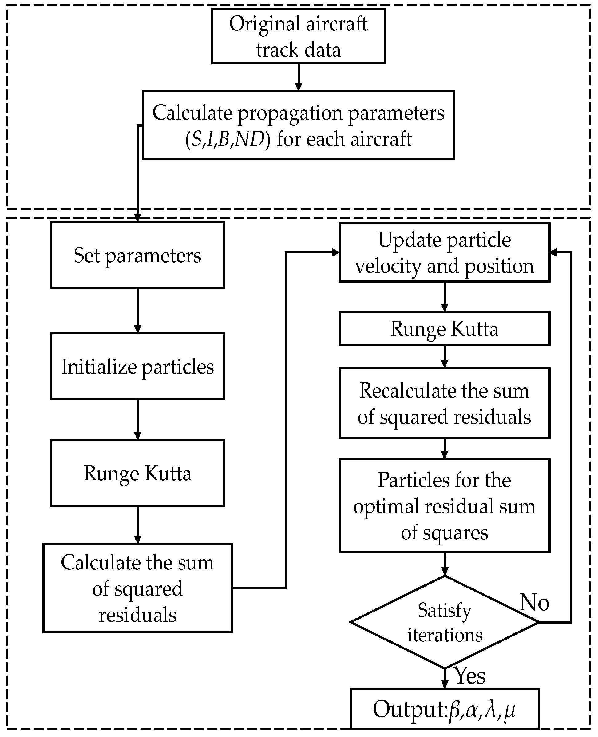
For differential equations of most propagation models, it is difficult to find their precise solutions. To solve the differential equations of a propagation model, the use of numerical algorithms certainly will generate errors, and the infection rate β and recovery rate α of different combinations will further affect the fitting result of real data. Thus, PSO is used to optimize the infection rate β and recovery rate α, which will control the fitting errors within a reasonable range. With improved PSO and the Runge–Kutta algorithm, the approximate solutions of differential equations are obtained. Basically, the differential equations are converted to an optimization problem, which is then solved using PSO. The specific flowchart is shown in Figure 5.

Figure 5.
The solution process of the propagation model.
First, based on numerous historical track data, a temporal network propagation model at the step length of 1 min is built according to the definition of the propagation mode, and the actual propagation process of all aircraft is calculated within the data range. Namely, the number of non-source aircraft per minute is S, the number of source aircraft is I, the number of aircraft leaving the airspace is ND, and the number of aircraft entering the airspace is B.
Then, the parameters of the propagation equation are solved for all aircrafts one by one. The initial parameters of a certain aircraft include the entering rate and leaving rate within a time period, and a set of randomly generated infection rate β and recovery rate α. The corresponding numerical solution is obtained using the 4-order Runge–Kutta algorithm, and the sum of squared residuals from this numerical solution to the real propagation process is determined. With the corresponding sum of squared residuals as a fitness function, the set of coefficients with the highest fitness from the real propagation process is further obtained using PSO and used as the propagation parameters of this aircraft.
For aircraft n, let the number of non-source aircraft in the actual propagation in the temporal network be , where is the number of non-source aircraft at time t for aircraft n; is the number of time periods of aircraft n in the temporal network. Let the number of source aircraft be , where is the number of source aircraft at time t for aircraft n. is the number of aircraft entering the airspace at time t for aircraft n. is the number of aircraft leaving the airspace at time t for aircraft n.
The entering rate of aircraft n at time t is defined as the proportion of aircraft entering the airspace at time accounting for the total number of aircraft:
Similarly, the leaving rate of aircraft n at time t is defined as the proportion of aircraft leaving the airspace at time accounting for the total number of aircraft:
Since the entering rate and leaving rate fluctuate little relative to the temporal network at period , the mean values of the entering rate and the leaving rate of this aircraft at each time period are used as the entering rate and leaving rate of this aircraft propagation model:
Let the function of residual sum of squares be p:
where is the function value at ; is the fitted value at .
Let the objective function of PSO be f:
When the sum of squared residuals between the fitted values and real values of S, I, B, and ND is the smallest, the fitting result is the best, so we output parameters .
4.3. Division of Propagation Ability
In the propagation model, the propagation threshold () measures whether a source aircraft can induce propagation. At , the number of source aircraft in the propagation process gradually increases, so propagation occurs in the network. At , propagation does not occur. Regardless of the values of infection rate and recovery rate, the numbers of source aircraft and non-source aircraft finally will stabilize, which is called the steady state. Our research on air traffic complexity propagation focuses on the changes in I and IND. The infection density and propagation velocity of source aircraft in the observed airspace can be determined by observing the changes in I. The infection density is defined as the proportion of source aircraft at the steady state accounting for all aircraft in the airspace. A larger infection density means the source aircraft are more influential for observation of airspace complexity. Moreover, when propagation occurs, the time from the start of propagation to the achievement of a steady state varies with the infection rate and the recovery rate, and a short time means the propagation velocity is faster. The IND at any time is the number of source aircraft leaving the airspace within the period from the start of propagation to the current time. A larger IND means the propagation delivers more higher-complexity aircraft to the nearby airspace.
In the propagation model, since the entering rate and leaving rate fluctuate little, the important influence factors of the propagation process are the infection rate and recovery rate. The state of the propagation process differs with the infection rate and recovery rate, which jointly decide the propagation process. To facilitate research on the propagation features of different aircraft, we adopt the infection rate and recovery rate as indices, and divide the aircraft using K-means clustering into three types: aircraft (Q1), (Q2), and (Q3) with high, moderate, and low propagation capability respectively.
5. Case Validation
With the real radar data from two days (1–2 November 2019) in the Shanghai region, the validation process is shown below.
5.1. Description of Real Data
At the step length of 1 min, the number of flights in the observed airspace within each time period was statistically analyzed (Figure 6).
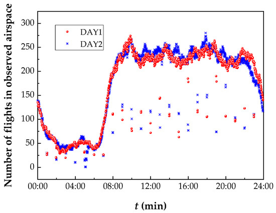
Figure 6.
Number of flights in observed airspace.
The number of flights in observed airspace fluctuates largely before 8:30 a.m. and after 10:30 p.m. To avoid large modeling errors due to severe fluctuation in the number of flights, we chose the radar data in the period from 8:30 a.m. to 10:30 p.m. The raw data contains flight number, speed, altitude, position coordinates, etc.
5.2. Calculated Results of Propagation Model Parameters
First, with 1 min as the step length, a temporal network was built with aircraft as nodes and between-aircraft proximity relations as edges. Second, the relative velocity , duration , network temporal-correlation coefficients , node temporal-correlation coefficient of each aircraft, and network temporal-correlation coefficient in this period were calculated. Third, the number of non-source aircraft S, number of source aircraft I, number of leaving aircraft ND, number of entering aircraft B, entering rate , and leaving rate every minute in the time effective network propagation model were computed. Finally, the set of parameters (infection rate and recovery rate ) with the smallest sum of squared residuals for each aircraft were determined using the Runge–Kutta algorithm and PSO (Figure 7). The average R2 of the propagation model is 0.917, indicating that the solved parameters can better describe the propagation process of air traffic complexity.
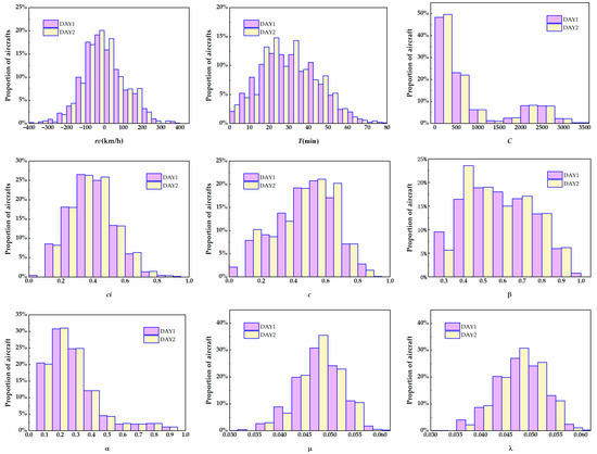
Figure 7.
Influencing factors and related parameters of the propagation model.
5.3. Results of Propagation Ability Division
With the propagation parameters (infection rate and recovery rate ) as obtained as the indices, all aircraft were clustered using the K-means algorithm. The propagation features of three types of aircraft were obtained (Table 1), including Q1, Q2, and Q3 aircraft with high, medium, and low propagation ability, respectively. Overall, the two-day propagation model characteristics are relatively close. The parameters for the second day were chosen for the explanation of the propagation process in this section.

Table 1.
Results of K-means algorithm.
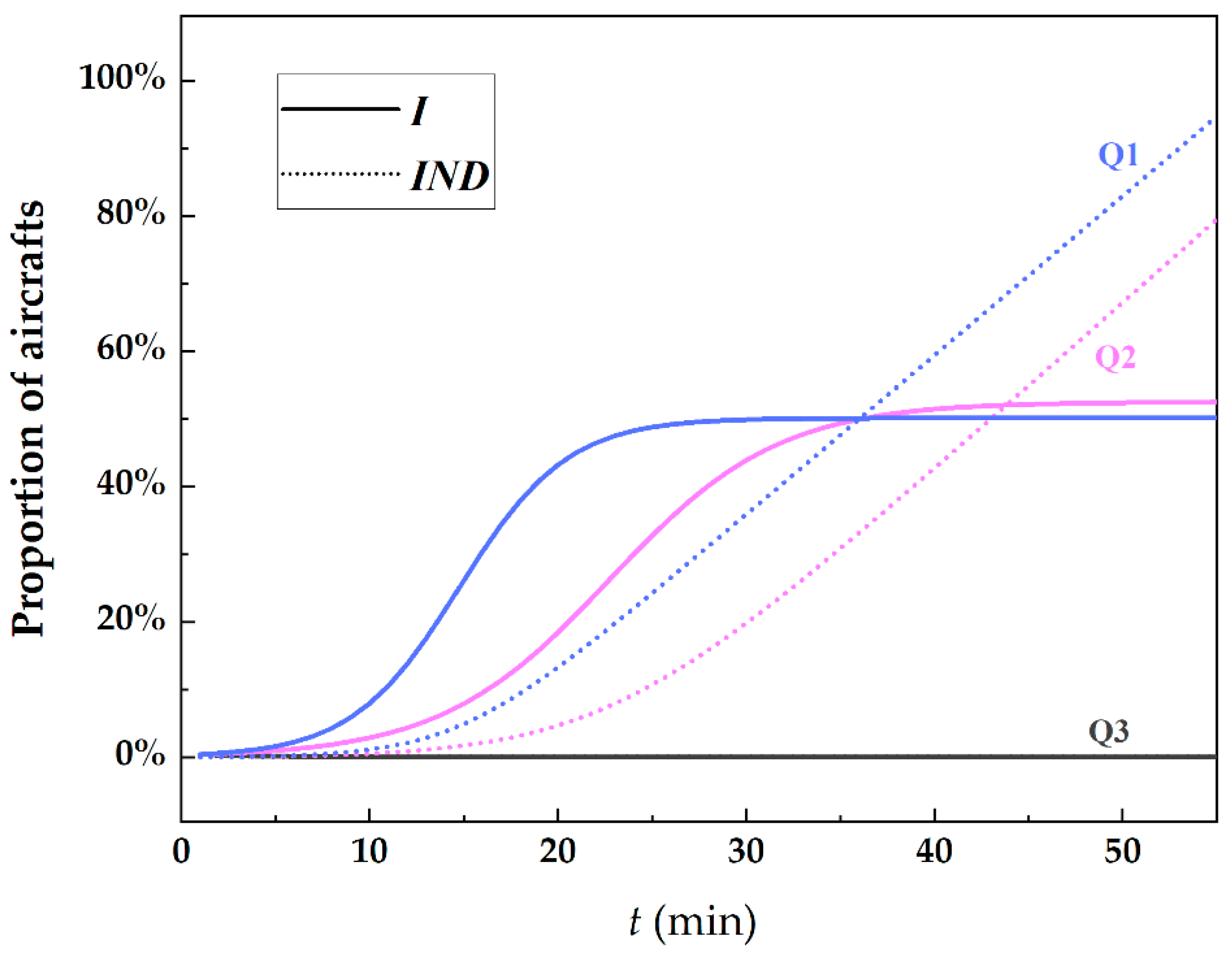
Figure 8 shows the actual propagation process of the aircraft closest to the clustering center in each of the three types, where solid lines show the source aircraft (I), and dot lines show the number of the source aircraft finally leaving from the observed airspace (IND). Clearly, Q1 aircraft after entering the airspace propagate at the fastest velocity among all three types. Moreover, the accumulative number of source aircraft leaving from the observed airspace is the largest from Q1 aircraft, which transport the most high-complexity source aircraft to nearby airspace. However, the infection density of Q1 aircraft is slightly lower than that of Q2 aircraft. The propagation velocity of Q2 aircraft after entering the sector is slightly slower than that of Q1 aircraft, but some Q2 aircraft leaving from the observed airspace become source aircraft, and the infection density of Q2 aircraft is the highest. Q3 aircraft do not induce propagation, or transport source aircraft to nearby airspace.
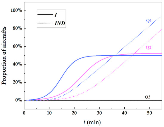
Figure 8.
The Propagation Process of Three Types of Aircraft with Different Propagation Capabilities.
5.4. Analytical Results of Influence Factors
The propagation process is jointly affected by the infection rate and recovery rate. For instance, the propagation threshold of a certain aircraft is , and is increased by one unit by adjusting a certain influence factor. At this moment, the change of infection rate is , the change of recovery rate is , so the new propagation threshold is . If , we cannot judge that the propagation threshold decreases, since the change of shall also be considered. If , then , and the threshold increases instead. Thus, in the regression analysis, if a certain influence factor only significantly affects either infection rate or recovery rate, it is hard to judge its effect on the other factor or to describe the effect of this significant factor in the propagation process. To clarify the concrete effect of the other factor on the propagation, we first built the connections of the influence factors with the infection rate and recovery rate, and then used the infection rate and recovery rate to describe the effects of the influence factors on propagation. Thus, the influence factors on propagation considered here are only the independent variables that significantly affect infection rate and recovery rate simultaneously.
The results of regression models are listed in Table 2, Table 3, Table 4, Table 5, Table 6 and Table 7. The normalization coefficient is the regression coefficient obtained after the independent variables and dependent variable are all normalized. After the normalization, the effects of dimensions and orders-of-magnitude are removed, which makes the independent variables comparable. Thus, the normalization coefficient is used to compare the magnitude of the effect of each independent variable on the dependent variable. The value of the normalization coefficient refers to the change of the dependent variable when the tested independent variable increases by every standard deviation. A larger absolute value of the normalization coefficient means the corresponding independent variable is more influential on the dependent variable [32].
Table 2.
The infection rate regression results of Q1 aircraft.
Table 3.
The recovery rate regression results of Q1 aircraft.
Table 4.
The infection rate regression results of Q2 aircraft.
Table 5.
The recovery rate regression results of Q2 aircraft.
Table 6.
The infection rate regression results of Q3 aircraft.
Table 7.
The recovery rate regression results of Q3 aircraft.
- Aircraft with high propagation capability (Q1)
The infection rate regression results of Q1 aircraft are listed in Table 2. The significant variables (Sig < 0.05) include the duration and the node temporal-correlation coefficients, with normalization coefficients of −0.185 and 0.125, respectively. Thus, duration negatively affects, and the node temporal-correlation coefficient positively affects the infection rate of Q1 aircraft. The recovery rate regression results of Q1 aircraft are listed in Table 3. The significant variables (Sig < 0.05) include the duration and the node temporal-correlation coefficient, with normalization coefficients of −0.424 and 0.088, respectively. Thus, duration negatively affects and the node temporal-correlation coefficient positively affects the recovery rate of Q1 aircraft.
Figure 9 shows the propagation process of Q1 aircraft after the duration or the node temporal-correlation coefficient is adjusted by one standard deviation. As the duration is prolonged, the infection rate and recovery rate both decrease, and the absolute value of change in the recovery rate is larger, so the corresponding propagation velocity, infection density, and IND all increase. These results suggest after the duration of Q1 aircraft is prolonged, the generation of proximity relations in the observed airspace is quickened, which intensifies the potential workload of air traffic controllers. When the propagation becomes steady, the number of aircraft with increased complexity due to the impact of propagation increases. In the meantime, the effect on the complexity in nearby airspace is stronger. As the node temporal-correlation coefficient is increased, the infection rate and recovery rate both rise, and the absolute value of change in the infection rate is larger, so the corresponding propagation velocity, infection density, and IND all decline. Namely, the speed of proximity relation generation, and the numbers of the affected aircraft in the observed airspace and nearby airspace both decrease.

Figure 9.
(a) I of Q1 when T increase or decrease by one standard deviation; (b) IND of Q1 when T increase or decrease by one standard deviation; (c) I of Q1 when ci increase or decrease by one standard deviation; (d) IND of Q1 when ci increase or decrease by one standard deviation.
- 2.
- Aircraft with medium propagation capability (Q2)
The infection rate regression results of Q2 aircraft are listed in Table 4. The significant variables (Sig < 0.05) include the duration and the clustering degree, with normalization coefficients of −0.143 and −0.235, respectively. Thus, duration and clustering degree both negatively affect the infection rate of Q2 aircraft, and the clustering degree is slightly more influential. The recovery rate regression results of Q2 aircraft are listed in Table 5. The significant variables (Sig < 0.05) include the duration and the clustering degree, with normalization coefficients of −0.127 and −0.233, respectively. Thus, duration and clustering degree both negatively affect the recovery rate of Q2 aircraft, and the clustering degree is slightly more influential.
Figure 10 shows the propagation process of Q2 aircraft after the duration or when the clustering degree is adjusted by one standard deviation. As the duration is prolonged, the infection rate and recovery rate both decrease, and the absolute value of change in the infection rate is larger, so the corresponding propagation velocity and IND decrease, whereas the infection density is basically unchanged. It is indicated after the duration of Q2 aircraft is prolonged, the speed of proximity relation generation is decelerated, the number of high-complexity aircraft transported to nearby airspace is smaller, but the number of affected aircraft in the observed airspace is stable. As the clustering degree C is increased, the infection rate and recovery rate both decrease, and the absolute value of change in the infection rate is larger. The corresponding propagation velocity decreases within 30 min, and increases after 30 min, whereas the infection density increases, and IND is basically unchanged. It is suggested after the clustering degree of Q2 aircraft is increased, the proximity relation generation speed is first decelerated and then quickened. Finally, the number of affected aircraft in the observed airspace increases, but the nearby airspace is basically unaffected. Thus, shortening the operation interval of Q2 aircraft can temporarily alleviate traffic pressure on controllers in practice.
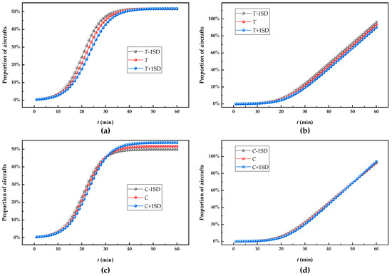
Figure 10.
(a) I of Q2 when T increase or decrease by one standard deviation; (b) IND of Q2 when T increase or decrease by one standard deviation; (c) I of Q2 when C increase or decrease by one standard deviation; (d) IND of Q2 when C increase or decrease by one standard deviation.
- 3.
- Aircraft with low propagation capability (Q3)
The infection rate regression results of Q3 aircraft are listed in Table 6. The significant variable (Sig < 0.05) includes velocity, with a normalization coefficient of −0.374. Thus, velocity negatively affects the infection rate of Q3 aircraft. The recovery rate regression results of Q3 aircraft are shown in Table 7. No significant influence factor is found.
Since no influence factor can significantly affect both infection rate and recovery rate of Q3 aircraft, the propagation process of Q3 aircraft cannot be analyzed using the above influence factors.
6. Conclusions
In order to gain a deeper understanding of the kinetic process of air traffic complexity propagation, a modeling and solution method based on complex network dynamics is proposed. The results show that the combination of Runge–Kutta and particle swarm optimization is effective in solving the propagation model of air traffic complexity, and the error is small. Since the effects of computation errors on the propagation process were alleviated, the propagation process modeled here is closer to actual situations.
Through the analysis of the propagation characteristics, the quantitative influence of the actual operation of air traffic controllers on the propagation process is obtained. Thus, according to the effects of different influence factors on the propagation process, the workloads on air traffic controllers can be dynamically adjusted in future research, which offers a feasible clue to balance the traffic flow pressures among different sectors. It should be noted that the influencing factors are only selected from the perspective of practical operation, the R2 of multiple linear regression still has room for improvement, and more influencing factors need to be further studied in the future. This model provides a feasible way to explore the complexity evolution mechanism and control method.
Author Contributions
Conceptualization, H.W. and P.X.; writing—original draft preparation, P.X.; writing—review and editing, F.Z.; supervision, H.W. All authors have read and agreed to the published version of the manuscript.
Funding
This research was funded by Key Program of Tianjin Science and Technology Plan, grant number 21JCZDJC00840 and National Natural Science Foundation of China, grant number U1833103.
Conflicts of Interest
The authors declare no conflict of interest.
References
- Schmidt, D.K. On modeling ATC workload and sector capacity. J. Aircr. 1976, 13, 531–537. [Google Scholar] [CrossRef]
- Hurst, M.W.; Rose, R.M. Objective job difficulty, behavioral response, and sector characteristics in air route traffic control centers. Ergonomics 1978, 21, 697–708. [Google Scholar] [CrossRef]
- Netjasov, F.; Janic, M.; Tosic, V. Developing a generic metric of terminal airspace traffic complexity. Transportmetrica 2011, 7, 369–394. [Google Scholar] [CrossRef]
- Prevot, T.; Lee, P.U. Trajectory-based complexity (TBX): A modified aircraft count to predict sector complexity during trajectory-based operations. In Proceedings of the IEEE/AIAA 30th Digital Avionics Systems Conference, Seattle, WA, USA, 16–20 October 2011. [Google Scholar]
- Lee, K.; Feron, E.; Pritchett, A. Describing airspace complexity: Airspace response to disturbances. J. Guid. Control Dyn. 2009, 32, 210–222. [Google Scholar] [CrossRef]
- Lee, K.; Feron, E.; Pritchett, A. Air traffic complexity: An input-output approach. In Proceedings of the 2007 American Control Conference, New York, NY, USA, 9–13 July 2007. [Google Scholar]
- Lyons, R. Complexity analysis of the next gen air traffic management system: Trajectory based operations. Work 2012, 41, 4514–4522. [Google Scholar] [CrossRef]
- Prandini, M.; Piroddi, L.; Puechmorel, S. Toward air traffic complexity assessment in new generation air traffic management systems. IEEE Trans. Intell. Transp. Syst. 2011, 12, 809–818. [Google Scholar] [CrossRef]
- Prandini, M.; Putta, V.; Hu, J. Air traffic complexity in future Air Traffic Management systems. J. Aerosp. Oper. 2012, 1, 281–299. [Google Scholar] [CrossRef]
- Rocha, E.C. Dynamics of air transport networks: A review from a complex systems perspective. Chin. J. Aeronaut. 2017, 2, 7–16. [Google Scholar] [CrossRef]
- Sun, X.Q.; Wandelt, S. Robustness of air transportation as complex networks: Systematic review of 15 years of research and outlook into the future. Sustainability 2021, 13, 6446. [Google Scholar] [CrossRef]
- Hossain, M.M.; Alam, S.; Symon, F.; Blom, H. A Complex Network Approach to Analyze the Effect of Intermediate Waypoints on Collision Risk Assessment. Air Traffic Control Q. 2014, 22, 87–114. [Google Scholar] [CrossRef]
- Hossain, M.M.; Alam, S. A complex network approach towards modeling and analysis of the Australian Airport Network. J. Air Transp. Manag. 2017, 60, 1–9. [Google Scholar]
- Complexity Metrics for ANSP Benchmarking Analysis. Available online: https://www.eurocontrol.int/publication/complexity-metrics-air-navigation-service-providers (accessed on 1 April 2006).
- Wang, H.Y.; Xu, X.H.; Zhao, Y.F. Empirical analysis of aircraft clusters in air traffic situation networks. Proc. Inst. Mech. Eng. Part G J. Aerosp. Eng. 2017, 231, 1718–1731. [Google Scholar] [CrossRef]
- Wang, H.Y.; Song, Z.Q.; Wen, R.Y. Modeling air traffic situation complexity with a dynamic weighted network approach. J. Adv. Transp. 2018, 1, 1–15. [Google Scholar] [CrossRef]
- Holme, P.; Saramäki, J. Temporal networks. Phys. Rep. 2012, 519, 97–125. [Google Scholar] [CrossRef]
- Holme, P. Modern temporal network theory: A colloquium. Eur. Phys. J. B 2015, 88, 1–30. [Google Scholar] [CrossRef]
- Rebollo, J.J.; Balakrishnan, H. Characterization and prediction of air traffic delays. Transp. Res. Part C Emerg. Technol. 2014, 44, 231–241. [Google Scholar] [CrossRef]
- Sismanidou, A.; Tarradellas, J.; Suau-Sanchez, P. The uneven geography of us air traffic delays: Quantifying the impact of connecting passengers on delay propagation. J. Transp. Geogr. 2022, 98, 103260. [Google Scholar]
- Balcan, D.; Colizza, V.; Goncalves, B.; Hu, H.; Ramasco, J.J.; Vespignani, A. Multiscale mobility networks and the large scale spreading of infectious diseases. Proc. Natl. Acad. Sci. USA 2009, 106, 21484–21489. [Google Scholar] [CrossRef]
- Balcan, D.; Hu, H.; Goncalves, B.; Bajarid, P.; Poletto, C.; Ramasco, J.J.; Paolotti, D.; Perra, N.; Tizzoni, M.; Broeck, W.V.D.; et al. Seasonal transmission potential and activity peaks of the new influenza A (H1N1): A Monte Carlo Likelihood analysis based on human mobility. BMC Med. 2009, 7, 45. [Google Scholar] [CrossRef]
- Fleurquin, P.; Ramasco, J.J.; Eguiluz, V.M. Systemic delay propagation in the US airport network. Sci. Rep. 2013, 3, 1159. [Google Scholar] [CrossRef]
- Pyrgiotis, N.; Malone, K.M.; Odoni, A. Modelling delay propagation within an airport network. Transp. Res. 2013, 27C, 60–75. [Google Scholar] [CrossRef]
- Li, Q.; Jing, R. Characterization of delay propagation in the air traffic network. J. Air Transp. Manag. 2021, 94, 102075. [Google Scholar] [CrossRef]
- Zanin, M.; Belkoura, S.; Zhu, Y. Network analysis of chinese air transport delay propagation. Chin. J. Aeronaut. 2017, 30, 491–499. [Google Scholar] [CrossRef]
- Wang, Y.; Zheng, H.; Wu, F.; Chen, J.; Hansen, M. A Comparative Study on Flight Delay Networks of the USA and China. J. Adv. Transp. 2020, 8, 1–11. [Google Scholar] [CrossRef]
- Li, S.M.; Xie, D.F.; Zhang, X.; Zhang, Z.Y.; Bai, W. Data-Driven Modeling of Systemic Air Traffic Delay Propagation: An Epidemic Model Approach. J. Adv. Transp. 2020, 2020, 1–12. [Google Scholar] [CrossRef]
- Cai, Q.; Alam, S.; Duong, V.N. A Spatial-Temporal Network Perspective for the Propagation Dynamics of Air Traffic Delays. Engineering 2021, 7, 452–464. [Google Scholar] [CrossRef]
- Shao, W.; Prabowo, A.; Zhao, S.; Koniusz, P.; Salim, F.D. Predicting flight delay with spatio-temporal trajectory convolutional network and airport situational awareness map. Neurocomputing 2022, 472, 280–293. [Google Scholar] [CrossRef]
- Jiang, J.L.; Fang, H.; Li, S.Q.; Li, W.M. Identifying important nodes for temporal networks based on the ASAM model. Phys. A: Stat. Mech. Its Appl. 2022, 586, 126455. [Google Scholar] [CrossRef]
- Maulud, D.; Abdulazeez, A.M. A review on linear regression comprehensive in machine learning. J. Appl. Sci. Technol. Trends 2020, 1, 140–147. [Google Scholar] [CrossRef]


Publisher’s Note: MDPI stays neutral with regard to jurisdictional claims in published maps and institutional affiliations. |
© 2022 by the authors. Licensee MDPI, Basel, Switzerland. This article is an open access article distributed under the terms and conditions of the Creative Commons Attribution (CC BY) license (https://creativecommons.org/licenses/by/4.0/).