An Improved Innovation Adaptive Kalman Filter for Integrated INS/GPS Navigation

Abstract

The performance of transportation systems has been greatly improved by the rapid development of connected and autonomous vehicles, of which high precision and reliable positioning is a key technology. An improved innovation adaptive Kalman filter (IAKF) is proposed to solve the vulnerability of Kalman filtering (KF) in challenging urban environments during integrated navigation. First, the algorithm uses the innovation to construct a chi-squared test to determine the abnormal measurement noise; on this basis, the update method of the measurement noise variance matrix is improved, and the measurement noise variance matrix is adaptively updated by the difference between the current innovation and the mean value of the innovation when the measurement data is abnormal so as to reflect the impact degree of the current abnormal measurement data, thus suppressing the filtering divergence and improving the positioning accuracy. The experimental results show that the proposed algorithm can well suppress the filtering divergence when the measurement data are disturbed. The results demonstrate that the algorithm in this paper has improved adaptiveness and stability and provides a novel idea for the development of an intelligent traffic positioning system.

1. Introduction

In recent years, global research on the application of intelligent transportation systems has developed rapidly [1,2]. Connected and autonomous vehicle (CAV) technology has quickly become a key component of intelligent transportation systems and an important pillar of smart city development [3]. CAV systems can not only provide information on the overall current road status, but also help vehicles choose the optimal path, which improves the operational efficiency and management of intelligent transportation. Considering the inherent defects such as high vehicle node movement speed and poor network stability in the Internet of Vehicles environment, higher requirements are put forward for the accuracy, stability and wide accessibility of vehicle positioning [4].

The positioning function of the Internet of Vehicles is mainly realized by the Global Navigation Satellite System (GNSS), Inertial System, and cameras. GNSS has the advantage of all-weather and high-precision positioning but has the disadvantage that the signal is easily blocked and interfered with [5]. The Inertial Navigation System (INS) does not rely on external information for autonomous navigation, which has the advantages of high short-term accuracy and strong reliability but has the disadvantage of the rapid accumulation of errors over time [6]. At present, multi-sensor information fusion technology is developing rapidly [7,8], and the positioning of vehicles in practical applications usually adopts integrated INS/GNSS navigation [9,10] and information fusion through a Kalman filter (KF), which can achieve complementary advantages and not only improve navigation accuracy but also improve the overall reliability of the system.

The standard KF requires an accurate mathematical model and the corresponding statistical characteristics of the system noise and measurement noise to be known accurately in advance. In practice, system modeling errors, as well as inaccurate measurement noise and system noise during navigation, can cause the standard KF accuracy to degrade and even diverge in severe cases. In order to overcome these issues, adaptive algorithms are widely used [11,12,13]. Adaptive filters estimate and correct noise statistical properties and model parameters online while using measurement data for filtering recursion to adapt to changes in system dynamics [14,15]. There are various methods of adaptive Kalman filtering, and the more commonly applied ones include the innovation-based adaptive filter [16], attenuation filter [17], and Sage–Husa adaptive filter [18]. Among them, the innovation-based adaptive filter can correct system noise and measurement noise at the same time; the attenuation filter can make better use of current measurement information and can correct errors caused by uncertain system models to a certain extent; the Sage-Husa adaptive filter can correct certain noise statistical characteristics, but when the dimension of the state variable estimated by the filter is high, the filter easily diverges.

Using the innovation sequences, a robust adaptive algorithm using sliding data windows to estimate the measurement noise in real time was proposed [19], which effectively suppresses the effects brought by data anomalies; however, the selection of the sliding window length relies on empirical selection. On the basis of the innovation sequences, considering that the current time measurements can more accurately reflect the characteristics of the noise, an attenuation factor is introduced to increase the weight of the current measurements, which can cope with the noise variation caused by environmental disturbances [20]. The key to attenuation filtering is to solve for the attenuation factor, which is used to reduce the use weight of old measurements while increasing the weight of new measurements [21,22,23], but usually only for correcting the filtering errors caused by model inaccuracies. However, the system process noise belongs to the inherent characteristics of the system and is generally not easy to change. Usually, as long as the settings are roughly accurate, there will not be too severe an impact on the filter accuracy, and too many adaptive parameters will lead to a reduction in filter stability.

The simplified Sage adaptive filter is an improved algorithm based on the KF, which can update the measurement noise variance matrix online while the state is estimated to achieve the adaptive effect [24]. The simplified Sage adaptive filter is robust but is computationally intensive and requires that the measurement noise variance must be a positive definite matrix, which is prone to scattering in integrated navigation systems with high dimensionality. A modified simplified Sage adaptive filter has been proposed by Ru [25], which does not restrict the positivity of the measurement noise variance matrix and ensures the stability of filtering while reducing the computation of the algorithm, but the improved algorithm is predicated on sacrificing some estimation accuracy. The adaptive Kalman filter algorithm based on reinforcement learning uses reinforcement learning to adaptively estimate the process noise covariance matrix. RL-AKF can significantly improve the positioning performance of integrated navigation when GNSS signals are not available [26]. However, the system process noise belongs to the inherent characteristics of the system, which are generally not easily changed. The method of adjusting the covariance matrix of the measurement vector by the scale factor obtained from the prediction residuals was proposed by Yan [27] so that the covariance matrix of the measurement vector keeps changing with the complex scene, and then the adaptive factor is calculated by the Mahalanobis distance to amplify the state prediction covariance matrix, which provides an innovative idea for the application of low-power, high-precision integrated navigation systems. Yang [28] proposed an improved adaptive attenuated square root unscented Kalman filter, which improved the algorithm’s adaptability to abruptly changing states by introducing an attenuation factor to adjust the filter gain in real time. However, the algorithm is mainly aimed at eliminating the interference of vibration on the measurement and obtaining accurate attitude parameters quickly. A method to establish the maximum a posteriori estimation and random weighted estimation of noise statistics was proposed [29], which can estimate and adjust the system noise statistics online, thus improving the filtering robustness. An adaptive filtering was proposed by [30] that can obtain the system noise estimate through the predefined fuzzy logic function and the chi-squared test value. However, it ignores the interference of the environment on the GPS signal.

In practical applications, a slight improvement in accuracy is secondary, and the number of adaptive parameters should be minimized to ensure the stability and reliability of filtering. The measurement noise is mainly caused by external factors, which are easy to change and have a great impact on the filtering accuracy. Constructing the adaptive factor by the residual vector is a typical adaptive filtering method [31], and the adaptive factor decreases as the residual increases, thus reducing the weight of the measurement data and achieving adaptive updating of the measurement noise variance matrix. However, adaptive factors are difficult to select for practical application. The conventional innovation adaptive filtering method is based on innovation to estimate the measurement noise and system noise so as to indirectly adjust the Kalman filter gain matrix, suppress the filter divergence, and improve the filter accuracy [32]. However, the method of using the average change value of the innovation covariance in the measurement update formula will reduce the sensitivity of the filter to the abnormal measurement value at the current moment and cannot sufficiently reduce the influence of the abnormal measurement value on the filtering.

Therefore, an improved innovation adaptive filtering algorithm (IAKF) was proposed in this paper for the shortcomings of attenuation filtering and conventional innovation adaptive filtering. Considering the Kalman filter update formulation, the gain matrix is mainly determined by the measurement noise variance matrix, the one-step prediction error variance matrix, and the system noise variance matrix. At the beginning of the filtering process, the filter’s estimation of the state is mainly dependent on the measurements of GNSS, so the measurement data anomalies have a great impact on the filtering estimation. When the filtering reaches stability, the filtering estimates tend to stabilize, and the innovation better describes the relationship between the filtered estimates and the actual measured values. Thus, the proposed algorithm judges the measurement data abnormality by means of the chi-squared test. When the measurement data are abnormal, the measurement noise variance matrix is adaptively updated by means of the difference between the current innovation and the average change value of the innovation covariance over time.

Different from the traditional AKF algorithm, considering that the stability of the filter and the inherent characteristics of the system noise is not easy to change, the algorithm in this paper focuses on the adaptive update research of the measurement noise. In addition, unlike the traditional method of adaptively updating the measurement noise matrix by innovation, the proposed algorithm reflects the influence of current measurement outliers on filtering by means of the difference between the current innovation and the mean value of innovation. The change value of the innovation covariance is added to the initial measurement noise matrix to scale up the measurement noise matrix to reduce the effect of outliers on filter estimation.

The paper is organized as follows. Section 2 contains the introduction and analysis of the update method of the standard KF and the influence of its related parameters on the filter update. In Section 3, a method of constructing a chi-squared test using the innovation series is proposed, an improved method of updating the measurement noise is given, and then the mathematical model of INS/GNSS integrated navigation is established. In Section 4, experimental results and analysis are given. Finally, the corresponding discussion and conclusions are provided in Section 5.

2. Kalman Filter and Its Parameter Analysis

The discrete Kalman filter system equation and measurement equation are as follows:

$$X_k={\Phi }_{k,k-1}{X}_{k-1}+{\Gamma }_{k,k-1}{W}_{k-1}$$

(1)

$$Z_k=H_k{X}_k+V_k$$

(2)

where $X_k$ is the state vector, ${\Phi }_{k,k-1}$ is the state transition matrix, ${\Gamma }_{k,k-1}$ is the matrix of noise driving, $W_{k-1}$ is the noise vector of the system, $Z_k$ is the measurement vector, $H_k$ denotes the measurement matrix, and $V_k$ is the measurement noise. $W_{k-1}$ and $V_k$ are uncorrelated and meet the following properties:

$$E[W_k]=0,E[V_k]=0,\mathrm{cov}[W_k,V_j]=E[W_k{V}_j^T]=0$$

(3)

$$\mathrm{cov}[W_k,W_j]=E[W_k{W}_j^T]=Q_k{\delta }_{kj}$$

(4)

$$\mathrm{cov}[V_k,V_j]=E[V_k{V}_j^T]=R_k{\delta }_{kj}$$

(5)

where $Q_k$ is the system noise matrix, $R_k$ is the measurement noise matrix, and ${\delta }_{kj}$ is the Kronecker-$\delta$ function.

The update formula of the Kalman filter is shown below.

The one-step state predicting equation is as follows:

$${\stackrel{\wedge }{X}}_{k,k-1}={\Phi }_{k,k-1}{\stackrel{\wedge }{X}}_{k-1}$$

(6)

The error variance matrix of the one-step predicting method is as follows:

$$P_{k,k-1}={\Phi }_{k,k-1}{P}_{k-1}{\Phi }_{k,k-1}^T+{\Gamma }_{k-1}{Q}_{k-1}{{\rm I}}_{k-1}^T$$

(7)

The Kalman gain matrix is as follows:

$$K_k=P_{k,k-1}{H}_k^T{(H_k{P}_{k,k-1}{H}_k^T+R_k)}^{-1}$$

(8)

The state estimation equation is as follows:

$${\stackrel{\wedge }{X}}_k={\stackrel{\wedge }{X}}_{k,k-1}+K_k(Z_k-H_k{\stackrel{\wedge }{X}}_{k,k-1})$$

(9)

The estimation error variance matrix is as follows:

$$P_k=(I-K_k{H}_k)P_{k,k-1}$$

(10)

From Equations (7) and (8), it can be concluded that the size of the gain matrix $K_k$ is mainly affected by the system noise matrix $Q_{k-1}$ and the measurement noise matrix $R_k$. Therefore, in the Kalman filter update process, if the setting of the system noise matrix $Q_{k-1}$ is smaller than the actual noise distribution or the setting of the observed noise matrix $R_k$ is larger than the actual noise distribution, the gain matrix $K_k$ will be too small, resulting in a biased estimation due to the small uncertainty range of the true value of the state estimation. Conversely, too large a value of the gain matrix $K_k$ may lead to filter divergence.

As can be seen from Equation (9), if there are abnormal values in the measurement data, the system still uses the initialized measurement noise variance matrix without timely adjustment, and the abnormal measurement values will have an impact on the filtering results, resulting in the filtering convergence effect not being obvious or even causing filtering divergence. Therefore, if the observed noise matrix $R_k$ can be adaptively adjusted in the filtering process, the adaptability of the KF algorithm and the ability to suppress outliers will be greatly improved.

3. Methodology of Proposed Improved Innovation Adaptive Kalman Filter

3.1. Constructing a Chi-Squared Test Using the Innovation Series

The chi-squared test is a hypothesis testing method that counts the degree of deviation between the theoretical value and the actual value of the sample. The magnitude of the chi-squared test statistic is determined by the degree of deviation between the theoretically estimated value and the actual measurement value. The greater the degree of deviation between the two, the greater the chi-squared test statistic. When the chi-squared test value is zero, the theoretically estimated value is equal to the actual observed value.

The innovation reflects the relationship between the actual current measurement and the estimated values. In the case of optimal filtering, the measure is not disturbed, and the innovation sequence obeys the Gaussian white noise property with zero mean. When the environment interferes with the measurement noise abnormally, the zero-mean characteristic of the whole innovation will also be destroyed. Therefore, the chi-squared test established by the innovation sequence can be used to judge whether there are outliers.

First, the statistical tests are constructed using innovation as follows:

$$T_k=r_k^T{(H{P}_{k,k-1}{H}^T+R_k)}^{-1}{r}_k$$

(11)

where $r_k$ denotes the innovation, and it is calculated as follows:

$$r_k=Z_k-H_k{\stackrel{\wedge }{X}}_{k,k-1}$$

(12)

Outliers in the statistic are detected by the chi-squared test, which has the following test issues:

$$T_k\sim {\chi }^2(m,0)$$

(13)

where $m$ is the degree of freedom, that is, the dimension of the measurement information, and the decentralization parameter is zero. That is, $T_k$ follows a chi-squared distribution with m degrees of freedom.

By setting the appropriate quantile $a$, the test rejection domain is

$$W=\left\{T_k\ge {\chi }_a^2\left(n-1,0\right)\right\}$$

(14)

That is, the value in the test rejection area indicates that the actual value of the statistic deviates too much from the theoretical value, and the assumption does not hold. This means that it is considered that the zero-mean characteristic of innovation is lost, the measurement is abnormally interfered with, and abnormal values appear.

3.2. Improved Innovation-Based Measurement Noise Update Method

The expression for the innovation covariance in the filtered optimal case is

$$C_k=\left[r_k{r}_k^T\right]=H_k{P}_{k,k-1}{H}_k^T+R_k$$

(15)

The estimated value of the innovation covariance is generally obtained by the windowing method [33].

$$\stackrel{\wedge }{C_k}=\frac{1}{k-1}{\displaystyle \sum _{i=1}^k{r}_i{r}_i^T}$$

(16)

The traditional innovation adaptive filtering algorithm improves the filtering accuracy by updating the system noise variance matrix and the measurement noise variance matrix online [34].

$$\stackrel{\wedge }{R}={\stackrel{\wedge }{C}}_k-H{P}_{k,k-1}{H}^T$$

(17)

$${\stackrel{\wedge }{Q}}_k=\frac{1}{N}{\displaystyle \sum _{T-T_0}^k\Delta x_j^T+P_k+{\Phi }_{k,k-1}{P}_{k-1}}{\Phi }_{k,k-1}^T$$

(18)

While the system noise belongs to the inherent characteristics of the system, which are generally not easy to change, usually, as long as the settings are roughly accurate, the filtering accuracy will not have too great an impact. In practical applications, the stability of the filtering should be focused on. The measurement noise is mainly caused by external environmental factors, which have a large impact on the filtering accuracy; only the measurement noise variance matrix is adaptively updated in this paper. The improved measurement noise variance matrix update proposed in this paper is as follows:

$${\stackrel{\wedge }{R}}_k=\frac{(r_k-{\stackrel{\wedge }{r}}_k){(r_k-{\stackrel{\wedge }{r}}_k)}^T}{k}+R_k$$

(19)

$${\stackrel{\wedge }{r}}_k=\frac{1}{k}{\displaystyle {\sum }_{i=1}^k{r}_i}$$

(20)

where k is the current epoch. When the chi-squared test, established in Section 3.1, detects abnormal measurement data, the innovation covariance is used for a posteriori estimation, and the change value of the innovation covariance is added on the basis of the initial measurement noise. The $R_k$ is adjusted upwardly, and the gain matrix $K_k$ is decreased to reduce the influence of measurement data with outliers on the filter estimation. The update process is as follows.

The Kalman filter time update equation is

$${\stackrel{\wedge }{X}}_{k,k-1}={\Phi }_{k,k-1}{\stackrel{\wedge }{X}}_{k-1}$$

(21)

$$P_{k,k-1}={\Phi }_{k,k-1}{P}_{k-1}{\Phi }_{k,k-1}^T+{\Gamma }_{k-1}{Q}_{k-1}{{\rm I}}_{k-1}^T$$

(22)

When the chi-squared test detects a measurement abnormality, the measurement noise matrix is updated by Formula (19) and (20), and the Kalman filter measurement update formula takes the following form.

$$K_k^{*}=P_{k,k-1}{H}_k^T{(H_k{P}_{k,k-1}{H}_k^T+{\stackrel{\wedge }{R}}_k)}^{-1}$$

(23)

$${\stackrel{\wedge }{X}}_k={\stackrel{\wedge }{X}}_{k,k-1}+K_k^{*}(Z_k-H_k{\stackrel{\wedge }{X}}_{k,k-1})$$

(24)

$$P_k^{*}=(I-K_k^{*}{H}_k)P_{k,k-1}$$

(25)

This method of adaptively updating the measurement noise matrix $R_k$ by making the difference between the current innovation and the average change value of the innovation covariance can reflect the influence of the current abnormal measurement data and adjust the gain matrix $K_k$, thereby suppressing the filtering divergence and improving the filtering accuracy. The flowchart of the improved innovation adaptive Kalman filter algorithm is shown in Figure 1.

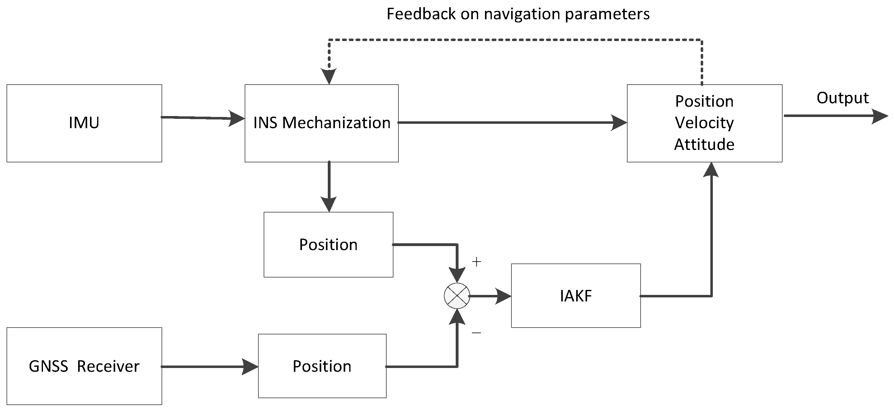
3.3. Mathematical Model of INS/GNSS Integrated Navigation

In this paper, the misalignment angle of the platform, the velocity error, the position error, and the zero bias of the gyro and accelerometer are selected to construct a 15-dimensional state vector. The state vector $X$ is listed below:

$$X={\left[\begin{array}{ccccccccccccccc}{\phi }_e& {\phi }_n& {\phi }_u& \delta V_e& \delta V_n& \delta V_u& \delta L& \delta \lambda & \delta h& {\epsilon }_x& {\epsilon }_y& {\epsilon }_z& {\nabla }_x& {\nabla }_y& {\nabla }_z\end{array}\right]}^T$$

(26)

The state equation of the continuous system is

$$X(t)=F(t)X(t)+G(t)W(t)$$

(27)

where $X(t)$ is the state vector, $F(t)$ is the transfer matrix of step, $G(t)$ is the matrix of noise driving, and $W(t)$ is the noise vector of the system.

Equation (27) after discretization processing is

$$X(k)=\Phi (k,k-1)X(k-1)+\Gamma (k-1)W(k-1)$$

(28)

where $\Phi (k,k-1)$ is the state transfer matrix, $\Gamma (k-1)$ is the noise matrix, and $W(k-1)$ is the system noise sequence.

The measurement equation is constructed by taking the difference between the three-dimensional position output by INS and GNSS as the measurement value.

$$Z(k)=[P_{INS}-P_{GNSS}]=\left[\begin{array}{c}{L}_{INS}-L_{GNSS}\\ {\lambda }_{INS}-{\lambda }_{GNSS}\\ h_{INS}-h_{GNSS}\end{array}\right]=H(k)X(k)+V(k)$$

(29)

The position information output by the INS consists of the actual position and the solution error of the INS, which can be written as the following formula:

$$\begin{array}{l}{L}_{INS}=L+\delta L_{INS}\\ {\lambda }_{INS}=\lambda +\delta {\lambda }_{INS}\\ h_{INS}=h+\delta h_{INS}\end{array}$$

(30)

where $L$, $\lambda$, and $h$ represent the actual latitude, longitude and altitude of the current vehicle, respectively. $\delta L_{INS}$, $\delta {\lambda }_{INS}$, $\delta h_{INS}$ represent the latitude, longitude and altitude errors of the INS solution output, respectively.

GNSS position information consists of two parts, the actual position and the position error of GNSS, which can be written as the following formula:

$$\begin{array}{l}{L}_{GNSS}=L+\delta L_{GNSS}\\ {\lambda }_{GNSS}=\lambda +\delta {\lambda }_{GNSS}\\ h_{GNSS}=h+\delta h_{GNSS}\end{array}$$

(31)

where $\delta L_{GNSS}$, $\delta {\lambda }_{GNSS}$, and $\delta h_{GNSS}$ represent the latitude, longitude and altitude errors of GNSS, respectively.

$H_k$ is defined as follows:

$$H_k=\left[\begin{array}{ccc}{0}_{3\times 6}& I_{3\times 3}& 0_{3\times 6}\end{array}\right]$$

(32)

$V_k$ is defined as follows:

$$V_k=\left[\begin{array}{ccc}{\eta }_L& {\eta }_{\lambda }& {\eta }_h\end{array}\right]$$

(33)

where ${\eta }_L$, ${\eta }_{\lambda }$ and ${\eta }_h$ represent the noise errors when the GNSS receiver acquires the current latitude, longitude and altitude, which are all Gaussian white noise.

Finally, the INS/GNSS loose integrated navigation model constructed in this paper is shown in Figure 2.

4. Experiment

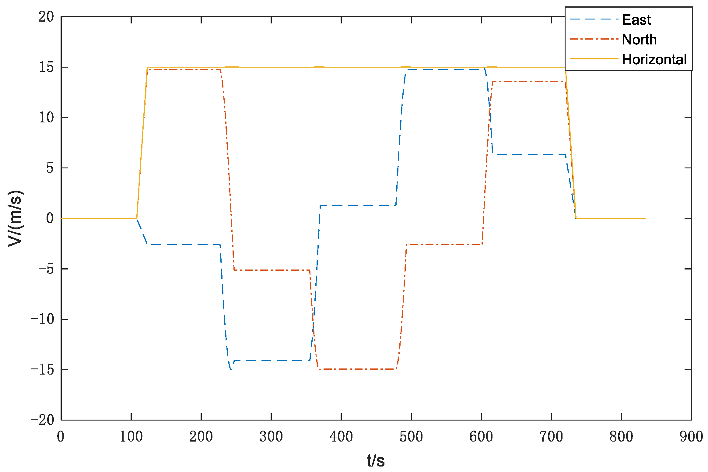
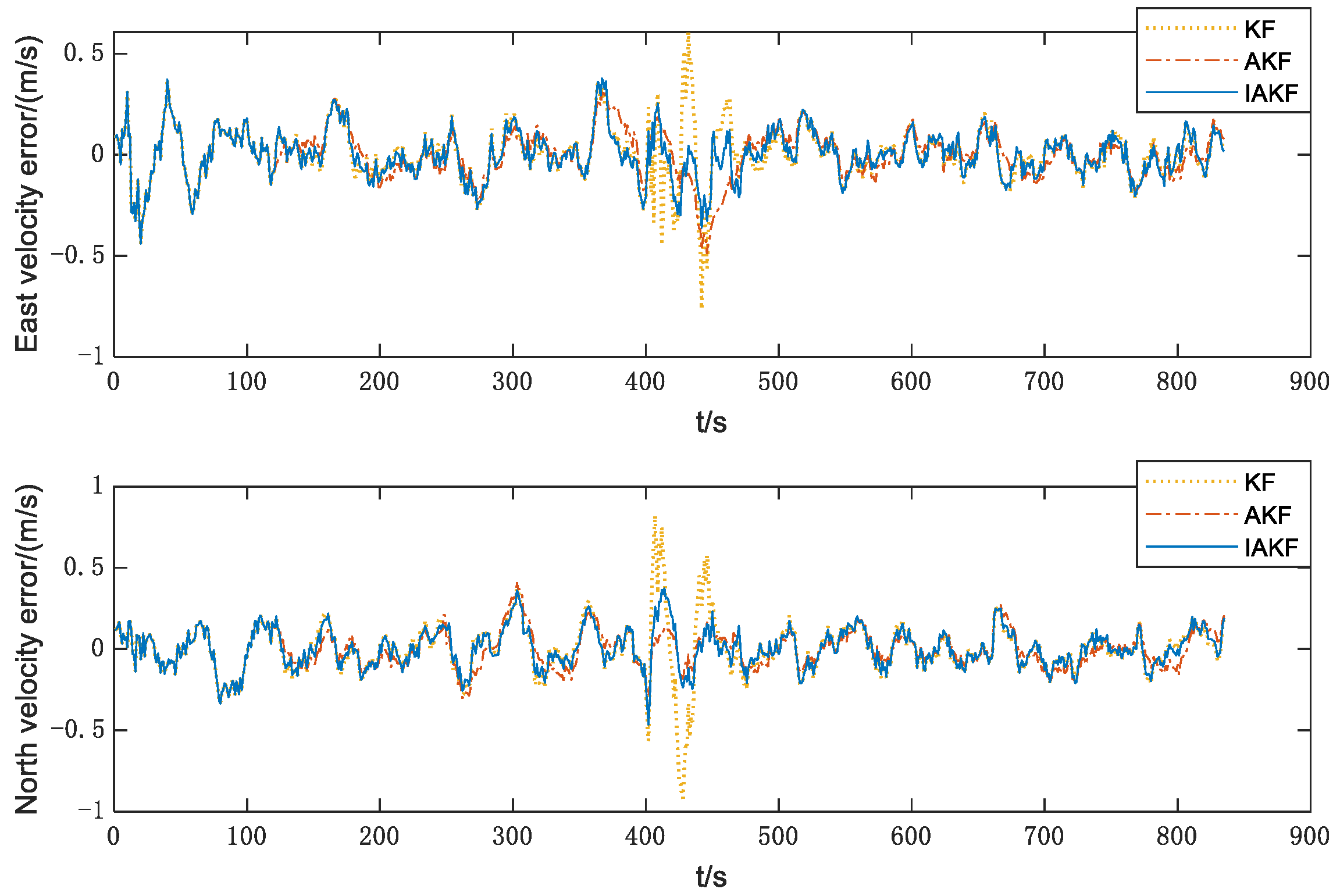
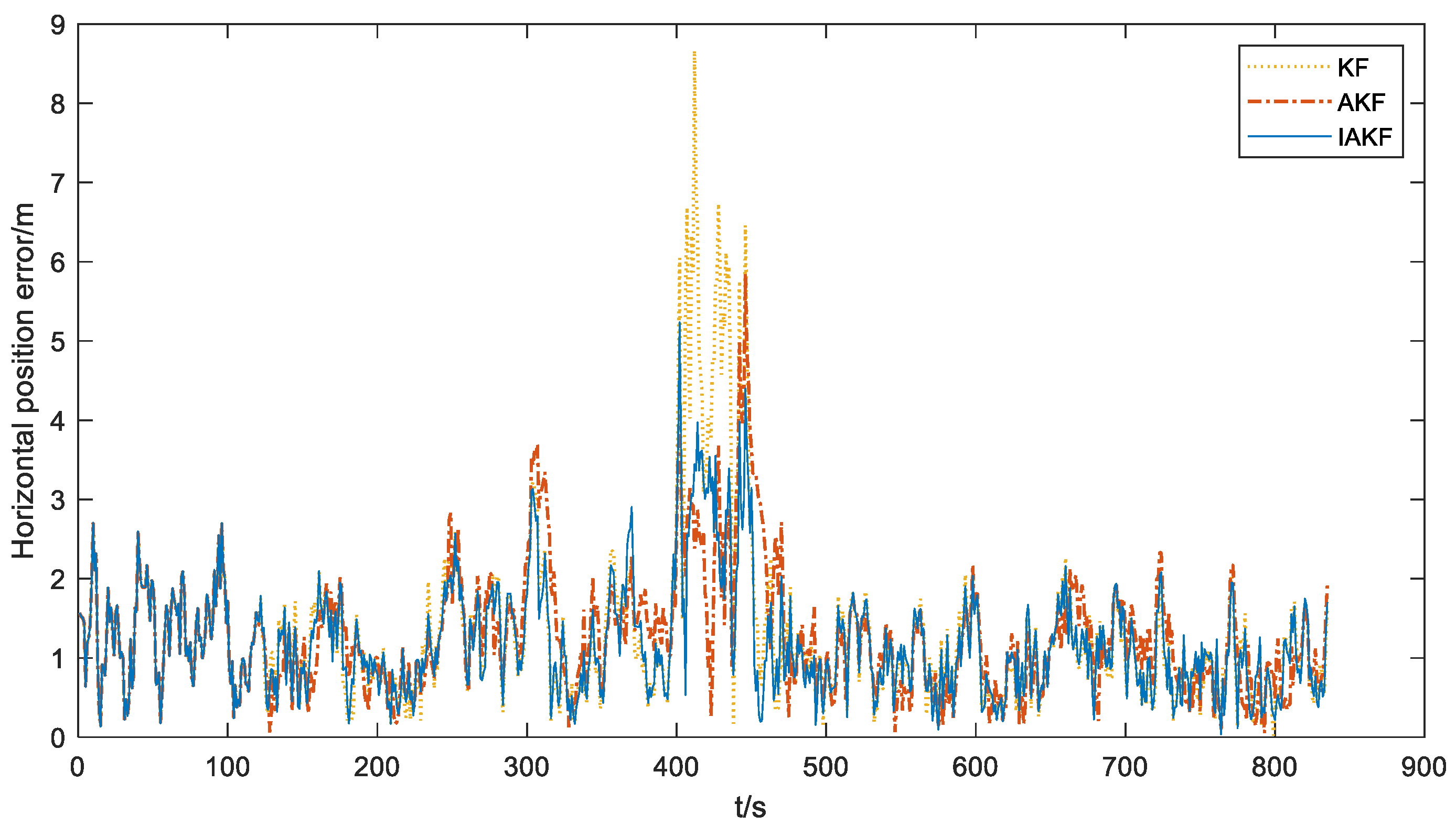
4.1. Simulation Experiment

To verify the effectiveness of the algorithm proposed in the article, a simulation experiment was first carried out, in which the performance of the IMU (inertial measurement unit) device is shown in

Table 1. IMU parameters.

IMU Parameter	Value
INS out frequency	100 Hz
Gyro bias	5°/h
Gyro angle random walk	0.5°/sqrt(h)
Accelerometer bias	400 ug

. The simulation experiment first simulates the track and velocity of the vehicle, as shown in Figure 3 and Figure 4, respectively.

From the track and velocity curve of the vehicle, it can be seen that the state of the vehicle includes acceleration, deceleration, turning and other conventional states.

The GPS positioning error is shown in Figure 5. The GPS signal is disturbed by the environment during the 400–450 s time period, and the positioning error becomes larger; that is, the measurement data is abnormal. The GPS positioning error statistics are shown in

Table 2. GPS positioning error statistics.

	Position Error (m)
	North	East	Horizontal
Mean	1.843	1.567	2.945
Max	16.75	16.942	24.382

.

It can be seen from Figure 5 and Table 2 that the GPS positioning error is relatively stable, but in the 400–450 s time period, the GPS signal is disturbed by the environment, resulting in abnormal measurements. The positioning error increases sharply, the fluctuation is large, and the maximum value of horizontal error reaches 24.382 m. Therefore, if the measurement noise matrix is not updated, the abnormal measurement will have a significant impact on the filtering, which will reduce the filtering accuracy and even cause the filtering to diverge.

In order to verify the effectiveness of the proposed algorithm in this paper, it is compared with the KF and traditional AKF algorithms, and the east and north velocity error curves, east and north position error curves and horizontal positioning error curves of INS/GNSS integrated navigation are output, as shown in Figure 6, Figure 7 and Figure 8.

It can be seen from the error curves in Figure 6, Figure 7 and Figure 8 that in the non-interference period, the errors of the KF, AKF and IAKF algorithms are almost identical, which is because the statistical characteristics of the noise are basically realistic, and the measurement data do not contain outliers according to the 95% chi-squared test. However, in the interference period, the environment interferes with the measurement information, and the zero-mean property of the innovation is invalid, so the KF algorithm has a large estimation error. The AKF algorithm suppresses the filter divergence by adaptively correcting the system noise matrix and the measurement noise matrix. However, the proposed algorithm reduces the influence of the outliers on the filtering estimation by increasing the measurement noise matrix when there are outliers in the measurement data. From Figure 6, Figure 7 and Figure 8, it can be seen that the IAKF is more effective than the AKF algorithm in suppressing filter divergence, although, in Figure 7, the AKF has a lower maximum error in the eastward position. In addition, the statistical analysis of the positioning errors of GPS, KF, AKF and this paper’s algorithm in the simulation experiment is carried out in this paper, as shown in

Table 3. Positioning error statistics of the simulation experiment.

	Error Mean (m)			Error Max (m)
	East	North	Horizontal	East	North	Horizontal
GPS	1.843	1.567	2.945	16.75	16.942	24.382
KF	0.950	0.717	1.316	7.839	5.692	8.668
AKF	0.836	0.765	1.279	3.707	5.463	5.845
IAKF	0.825	0.685	1.198	5.023	3.983	5.234

.

As can be seen from Table 3, the mean and maximum values of the positioning errors of the KF, AKF and the proposed algorithm are significantly reduced compared to those of GPS, which indicates that the integrated INS/GNSS navigation is more accurate and stable compared to GNSS positioning alone. At the same time, due to the adaptive update of the measurement noise variance matrix, the algorithm in this paper has a more obvious suppression effect on the measurement anomaly compared with the KF algorithm, in which the mean value of error is reduced by 8.97%, and the maximum value of error is reduced by 39.62%. In addition, compared with the traditional AKF, the proposed algorithm performs better in terms of both the mean value of error and the maximum value of error, which verifies the stability and adaptiveness of the IAKF algorithm.

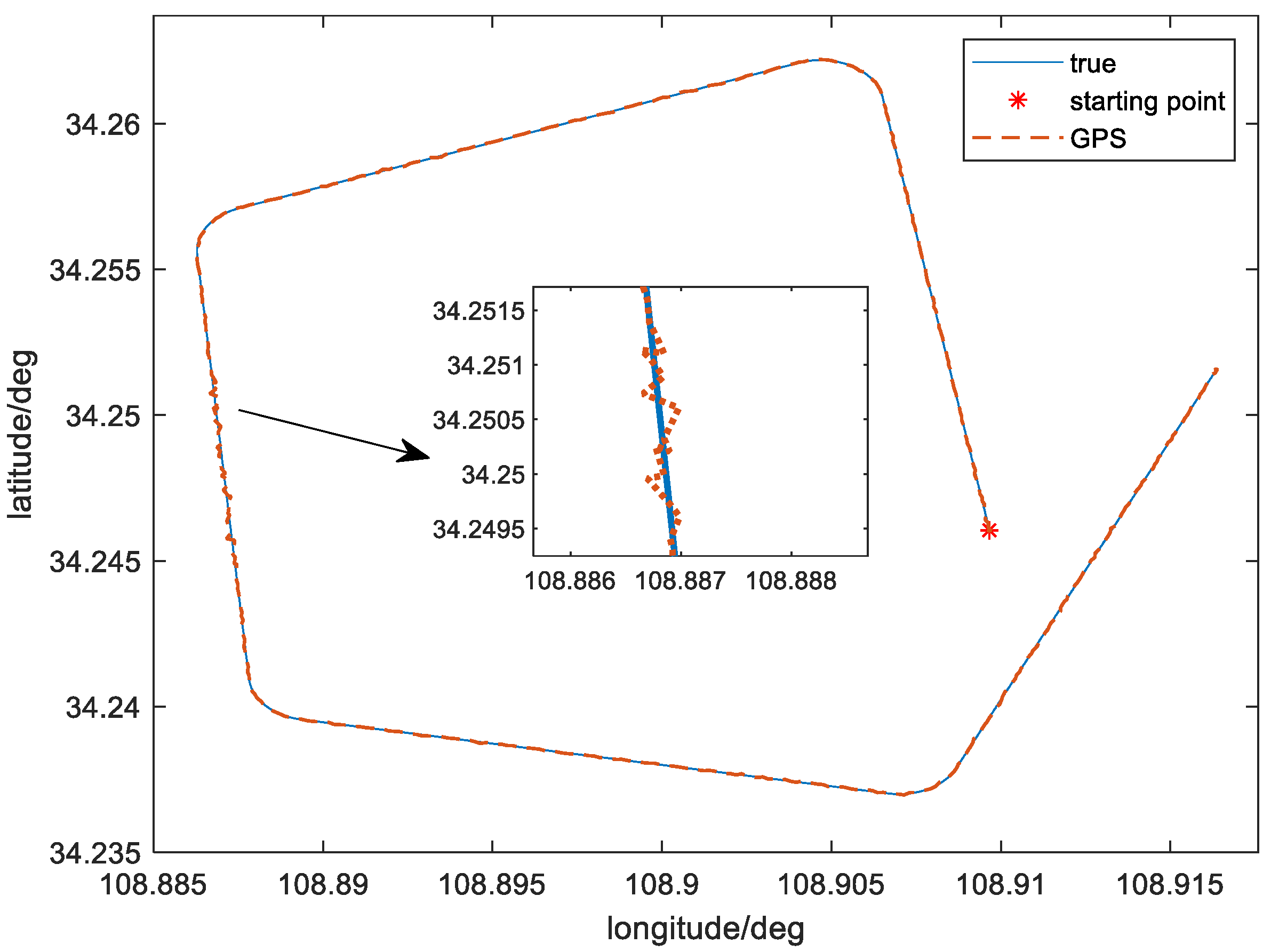
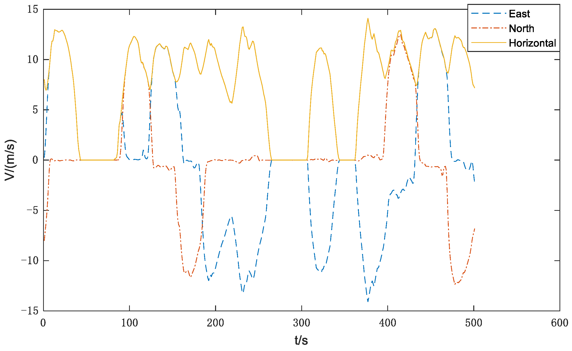
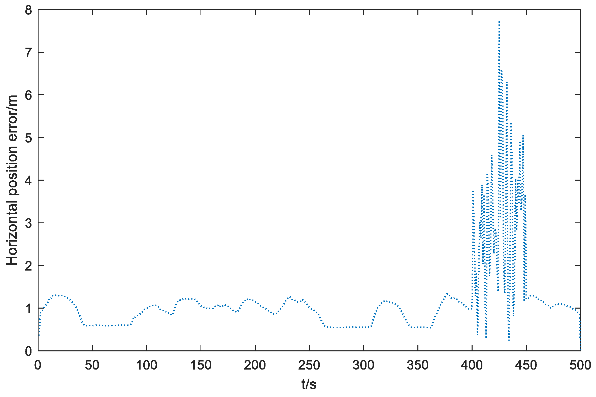
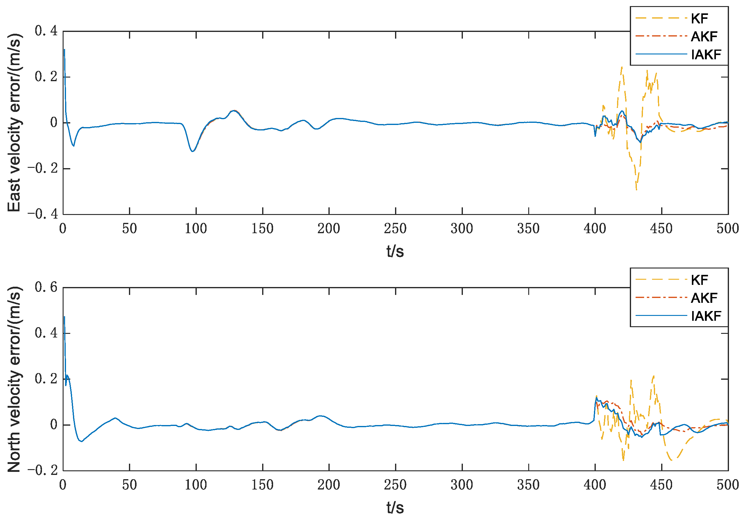
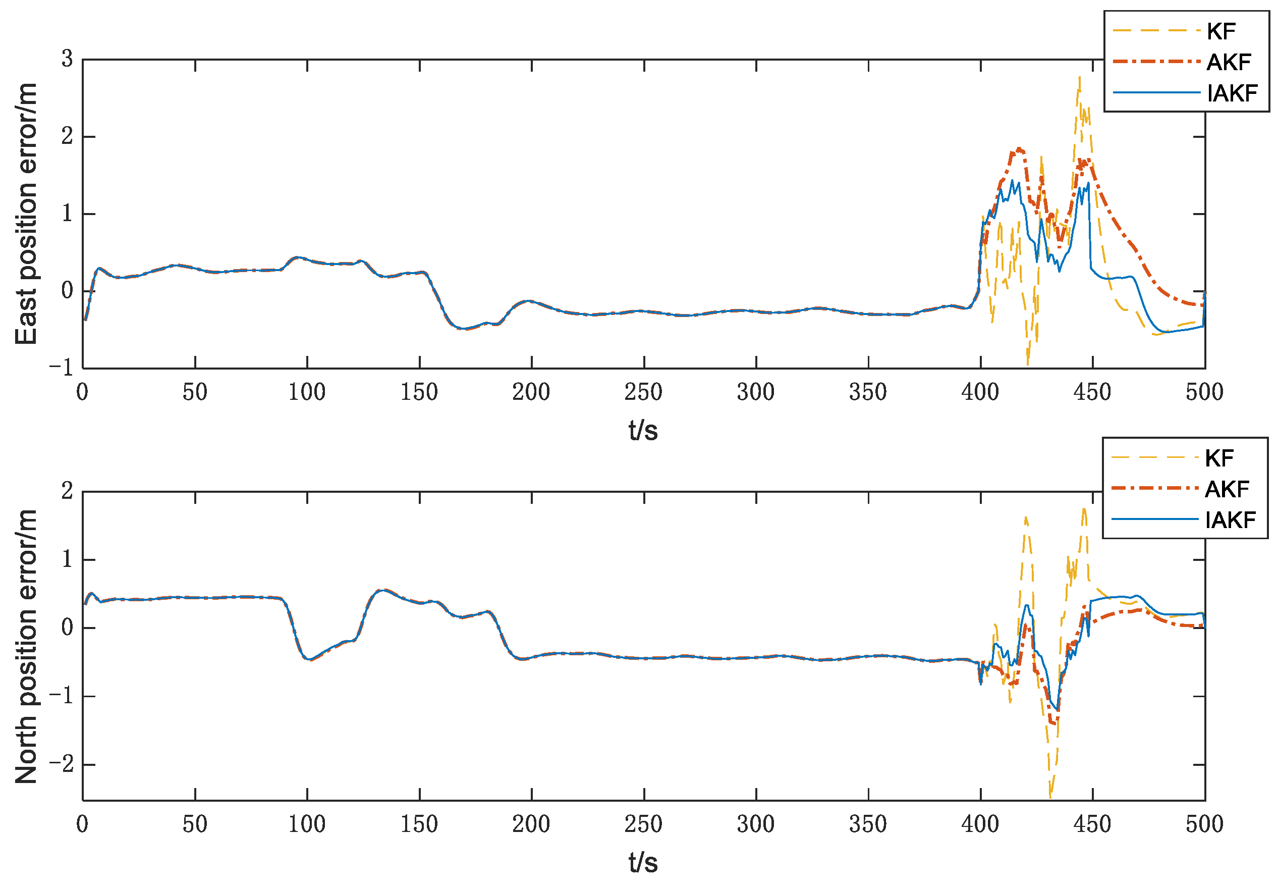
4.2. Real Vehicle Experiment

In order to verify the validity of the algorithm of the article, a set of real vehicle data was used for the experiment, and a 500 s segment of the data was selected. The IMU (FOG-KVH1775) was used, and the sampling frequency was 100 Hz; GPS adopted differential positioning, and the output frequency was 1 Hz. The data were output from the fiber-optic level integrated navigation system as the real value, with a theoretical error of 0.02 m or less, and the data were processed using MATLAB. The performance parameters of the IMU are shown in

Table 4. IMU parameters.

IMU Parameter	Value
INS out frequency	100 Hz
Gyro bias	0.5°/h
Gyro angle random walk	0.12°/sqrt(h)
Accelerometer bias	50 ug

, and the track and velocity of the vehicle are shown in Figure 9 and Figure 10.

The GPS positioning error curve is shown in Figure 11. To verify the effectiveness of the algorithm in this paper, interference errors, including Gaussian noise and irregular random errors, are added in the 400–450 s time period.

In order to verify the effectiveness of the proposed algorithm, it is compared with the KF and AKF, and the eastward and northward velocity error curves, eastward and northward position error curves, and horizontal positioning error curves of the integrated INS/GNSS navigation are output, as shown in Figure 12, Figure 13 and Figure 14.

From Figure 12 and Figure 13, it can be seen that IAKF performs better in terms of velocity error and position error, both in the east and north, and both are better than KF. As can be seen from Figure 14, the IAKF algorithm has a better suppression effect on horizontal position error and stronger filtering stability compared to the traditional AKF, which is due to the detection of anomalous measurements using the cardinality test of the innovation construction, which amplifies the gain matrix by updating measurement noise matrix, thus reducing the influence of the anomalous measurements on the filtering estimation.

Furthermore, the integrated INS/GNSS navigation tracks of different positioning methods are output in order to more intuitively demonstrate the positioning performance in this paper, as shown in Figure 15.

Figure 15 shows the localization performance of KF, AKF and IAKF. It can be clearly seen from the figure that the KF positioning track has obvious deviation in the road section where the GPS signal is interfered with. Although the performance of the AKF algorithm has improved, the track is still not ideal. Compared with the AKF algorithm, the track of the IAKF algorithm is closer to the real vehicle track, and the curve effect is smoother. Thus, the experimental results show that the algorithm in this paper can effectively suppress the filter divergence and improve the positioning accuracy. The error statistics of the article for the true vehicle experiment are shown in

Table 5. Position error statistics of different algorithms.

	Error Mean (m)			Error Max (m)
	East	North	Horizontal	East	North	Horizontal
GPS	0.5468	0.862	1.133	6.295	7.308	7.742
KF	0.355	0.444	0.595	2.776	2.524	3.026
AKF	0.394	0.391	0.593	1.855	1.400	2.002
IAKF	0.340	0.397	0.553	1.438	1.193	1.538

.

As shown in Table 5, IAKF reduces the mean value of error by 7.06% relative to KF, and the maximum value of error is reduced by 49.17%. In addition, compared with AKF, the algorithm in this paper performs better in terms of position error maximum. This shows that the proposed algorithm can not only effectively suppress the error divergence but also performs better compared with the traditional AKF.

5. Conclusions and Discussion

An improved innovation adaptive filtering algorithm is proposed for the vulnerability of integrated INS/GNSS navigation systems in challenging environments. First, the article analyzes the update formula of the Kalman filter, and the gain matrix is mainly determined by the measurement noise variance matrix, the one-step prediction error matrix and the system noise variance matrix. The measurement noise is easily affected by the environment and has a large impact on the filtering accuracy. In addition, the article reduces the number of adaptive parameters to ensure the stability and reliability of the filtering in practical applications.

Second, when the filtering is stable, the filtering estimation accuracy is improved, and the innovation is more descriptive of the relationship between the filtered estimates and the actual measurement data. Thus, the algorithm uses the innovation sequence to construct a chi-squared test to determine the measurement data anomaly, and when the measurement data is anomalous, the measurement noise variance matrix is adaptively updated by means of the difference between the current innovation and the average change in the innovation covariance.

The proposed algorithm is simulated and verified by the measured vehicle data by establishing the INS/GNSS integrated navigation system model and comparing the KF algorithm and AKF algorithm. The experimental results show that the proposed algorithm can suppress the filter divergence well when the measurement data is disturbed. Compared with the KF algorithm, the average positioning accuracy is improved by 7.06%. In addition, in terms of error maximum, the performance effect is better than AKF, which points to the fact that the proposed algorithm has good adaptability and robustness. The algorithm in this paper has a certain application value in the development of intelligent transportation systems, providing ideas to solve the inherent defects such as high movement speed of vehicle nodes and poor network stability in the CAV environment and meeting the requirements of accuracy, stability and wide accessibility of vehicle positioning in intelligent transportation.

In the future, we intend to combine the algorithm of this paper with attenuation filtering. In practical applications, model building is not perfect, and the filtering accuracy decreases with model errors. Attenuation filtering can increase the weight of current measurements to solve this problem. With the widespread use of integrated INS/GNSS navigation, low cost and high accuracy have become the focus of future research, and therefore, the articles will focus on this.

References

1. Gong, Y.; Feng, H.; Zhang, C. Research on the Development Strategy of the Internet of Vehicles. J. Phys. Conf. Ser. 2021, 1907, 012063. [Google Scholar] [CrossRef]
2. Ma, C.; Dai, G.; Zhou, J. Short-term traffic flow prediction for urban road sections based on time series analysis and LSTM_BILSTM method. IEEE Trans. Intell. Transp. Syst. 2022, 23, 5615–5624. [Google Scholar] [CrossRef]
3. Tian, D.; Wu, G.; Kanok, B. Performance Measurement Evaluation Framework and Co-Benefit\/Tradeoff Analysis for Connected and Automated Vehicles (CAV) Applications: A Survey. IEEE Intell. Transp. Syst. Mag. 2018, 10, 110–122. [Google Scholar] [CrossRef]
4. Min, H.; Song, X.; Cheng, C. Research on Development of Vehicle Collaborative Localization in Internet of Vehicles Environment. Unmanned Syst. Technol. 2021, 4, 8–14. [Google Scholar]
5. Liu, J.; Cao, C. Development status and trend of global navigation satellite system. J. Navig. Position 2020, 8, 22. [Google Scholar]
6. Ning, X.; Gui, M.; Xu, Y.; Bai, X.; Fang, J. INS/VNS/CNS integrated navigation method for planetary rovers. Aerosp. Sci. Technol. 2016, 48, 102–114. [Google Scholar] [CrossRef]
7. Qiao, D.; Zhang, Z.; Liu, F.; Sun, B. Location Optimization Model of a Greenhouse Sensor Based on Multisource Data Fusion. Complexity 2022, 2022, 3258549. [Google Scholar] [CrossRef]
8. Jiang, C.; Zhang, S.; Zhang, Q. Adaptive Estimation of Multiple Fading Factors for GPS/INS Integrated Navigation Systems. Sensors 2017, 17, 1254. [Google Scholar] [CrossRef]
9. Zhao, H.; Xiong, Z.; Shi, L.; Yu, F.; Liu, J. A robust filtering algorithm for integrated navigation system of aerospace vehicle in launch inertial coordinate. Aerosp. Sci. Technol. 2016, 58, 629–640. [Google Scholar] [CrossRef]
10. Davari, N.; Gholami, A.; Shabani, M. Performance Enhancement of GPS/INS Integrated Navigation System Using Wavelet Based De-noising method. AUT J. Electr. Eng. 2016, 48, 101–112. [Google Scholar]
11. Na, J.; Huang, Y.; Wu, X.; Su, S.; Li, G. Adaptive finite-time fuzzy control of nonlinear active suspension systems with input delay. IEEE Trans. Cybern. 2019, 50, 2639–2650. [Google Scholar] [CrossRef] [PubMed]
12. Jin, X.; Gong, W.; Kong, J. A Planar Flow-Based Variational Auto-Encoder Prediction Model for Time Series Data. Mathematics 2022, 10, 610. [Google Scholar] [CrossRef]
13. Chen, Q.; Tao, M.; He, X.; Tao, L. Fuzzy adaptive nonsingular fixed-time attitude tracking control of quadrotor UAVs. IEEE Trans. Aerosp. Electron. Syst. 2021, 57, 2864–2877. [Google Scholar] [CrossRef]
14. Yan, G.; Deng, Y. Review on Practical Kalman Filtering Techniques in Traditional Integrated Navigation System. Navig. Position Timing 2020, 7, 50–64. [Google Scholar]
15. Jiang, C.; Zhang, S.; Zhang, Q. A novel robust interval Kalman filter algorithm for GPS/INS integrated navigation. J. Sens. 2016, 2016, 3727241. [Google Scholar] [CrossRef]
16. Lin, X.; Liu, S.; Shi, Z. Multi-Sensor Signal Denoising Based on Adaptive Kalman Filter. Comput. Simul. 2022, 39, 507–511. [Google Scholar]
17. Pan, C.; Gao, J.; Li, Z.; Qian, N.; Li, F. Multiple fading factors-based strong tracking variational Bayesian adaptive Kalman filter. Measurement 2021, 176, 109139. [Google Scholar] [CrossRef]
18. Sun, L.; Hou, Y. Application of Sage-Husa adaptive filtering in trajectory prediction of moving obstacles. Manuf. Autom. 2022, 44, 73–75. [Google Scholar]
19. Li, W.; Chen, M.; Zhang, L.; Chen, R. Adaptive Kalman Filter Based on Innovation Sequence for SINS/DVL Integrated Navigation. J. Ordnance Equip. Eng. 2020, 41, 225–229. [Google Scholar]
20. Liu, Y.; Fan, X.; Lv, C.; Wu, J.; Li, L.; Ding, D. An innovative information fusion method with adaptive Kalman filter for integrated INS/GPS navigation of autonomous vehicles. Mech. Syst. Signal Process. 2018, 100, 605–616. [Google Scholar] [CrossRef]
21. Guo, S.; Wu, M.; Xu, J.; Li, J. Adaptive Fading Kalman Filter and Its Application in SINS Initial Alignment. Geomat. Inf. Sci. Wuhan Univ. 2018, 43, 1667–1672. [Google Scholar]
22. Wang, J.; Chen, X.; Yang, P. Adaptive H-infinite kalman filter based on multiple fading factors and its application in unmanned underwater vehicle. Isa Trans. 2021, 108, 295–304. [Google Scholar] [CrossRef] [PubMed]
23. Sun, B.; Zhang, Z.; Liu, S.; Yan, X.; Yang, C. Integrated Navigation Algorithm Based on Multiple Fading Factors Kalman Filter. Sensors 2022, 22, 5081. [Google Scholar] [CrossRef]
24. Yu, T.; Xu, A.; Fu, X.; Xie, Y.; Sun, W. An integrated navigation and positioning method of adaptive Kalman filtering. J. Navig. Position 2017, 5, 101–104. [Google Scholar]
25. Ru, G.; Feng, P.; Deng, Y. Adaptive filtering algorithm with switching state for GPS/INS. Eng. J. Wuhan Univ. 2015, 48, 574–579. [Google Scholar]
26. Gao, X.; Luo, H.; Ning, B.; Zhao, F.; Bao, L.; Gong, Y.; Xiao, Y.; Jiang, J. RL-AKF: An Adaptive Kalman Filter Navigation Algorithm Based on Reinforcement Learning for Ground Vehicles. Remote Sens. 2020, 12, 1704. [Google Scholar] [CrossRef]
27. Yan, P.; Jiang, J.; Zhang, F.; Xie, D.; Wu, J.; Zhang, C.; Tang, Y.; Liu, J. An Improved Adaptive Kalman Filter for a Single Frequency GNSS/MEMS-IMU/Odometer Integrated Navigation Module. Remote Sens. 2021, 13, 4317. [Google Scholar] [CrossRef]
28. Yang, Y.; Li, F.; Gao, Y.; Mao, Y. Multi-Sensor Combined Measurement While Drilling Based on the Improved Adaptive Fading Square Root Unscented Kalman Filter. Sensors 2020, 20, 1897. [Google Scholar] [CrossRef] [PubMed]
29. Gao, Z.; Mu, D.; Gao, S.; Zhong, Y.; Gu, C. Adaptive unscented Kalman filter based on maximum posterior and random weighting. Aerosp. Sci. Technol. 2017, 71, 12–24. [Google Scholar] [CrossRef]
30. Yang, C.; Guo, J.; Zhang, L.; Chen, Q. Fuzzy adaptive unscented Kalman filter integrated navigation algorithm using chi-square test. Control. Decis. 2018, 33, 81–87. [Google Scholar]
31. Qin, F.; Song, Z.; Wu, Z. Adaptive Robust Filter for INS/CNS/GNSS Integrated Navigation of the LEO Spacecraft. Aerosp. Control. Appl. 2017, 43, 55–59. [Google Scholar]
32. Zhou, X.; Zhang, H.; He, T.; Li, X. Research on adaptive Kalman filter algorithm for GPS/INS loosely coupled integrated navigation. J. Time Freq. 2020, 43, 222–230. [Google Scholar]
33. Xu, D.; He, R.; Shen, F.; Gai, M. Adaptive fading Kalman filter based on innovation covariance. Syst. Eng. Electron. 2011, 33, 2696–2699. [Google Scholar]
34. Xue, W.; Zhang, B.; Li, S. Application of New Information Adaptive Kalman Filter in Integrated Navigation. GNSS World China 2014, 39, 8–11. [Google Scholar]
Figure 1. Process of the improved innovation adaptive Kalman filter algorithm.
Sustainability 14 11230 g001
Figure 2. INS/GNSS loose integrated navigation model based on IAKF.
Sustainability 14 11230 g002
Figure 3. Vehicle track for simulation experiments.
Sustainability 14 11230 g003
Figure 4. Vehicle velocity for simulation experiments.
Sustainability 14 11230 g004
Figure 5. Horizontal positioning error of GPS.
Sustainability 14 11230 g005
Figure 6. East and north velocity error curves.
Sustainability 14 11230 g006
Figure 7. East and north position error curves.
Sustainability 14 11230 g007
Figure 8. Horizontal positioning error curves.
Sustainability 14 11230 g008
Figure 9. Track of vehicle.
Sustainability 14 11230 g009
Figure 10. Velocity of vehicle.
Sustainability 14 11230 g010
Figure 11. GPS positioning error curve.
Sustainability 14 11230 g011
Figure 12. East and north velocity errors.
Sustainability 14 11230 g012
Figure 13. East and north position errors.
Sustainability 14 11230 g013
Figure 14. Horizontal position errors.
Sustainability 14 11230 g014
Figure 15. Track comparison of different algorithms.
Sustainability 14 11230 g015