Article

Impact of Block Spatial Optimization and Vegetation Configuration on the Reduction of PM2.5 Concentrations: A Roadmap towards Green Transformation and Sustainable Development

1
School of Architecture, Southeast University, Nanjing 210096, China
2
Jiangsu Collaborative Innovation Center for Building Energy Saving and Construction Technology, Jiangsu Vocational Institute of Architectural Technology, Xuzhou 221000, China
*
Author to whom correspondence should be addressed.
Sustainability 2022, 14(18), 11622; https://doi.org/10.3390/su141811622
Submission received: 14 June 2022 / Revised: 5 September 2022 / Accepted: 6 September 2022 / Published: 16 September 2022
(This article belongs to the Special Issue Energy Economics and Energy Policy towards Sustainability)

Abstract

:
The article aims to reduce PM2.5 concentration by improving the spatial comfort of blocks and the vegetation configuration. It mainly analyzes the impact of the following five aspects on the PM2.5 concentration distribution in blocks, including different angles between the prevailing wind direction and blocks, different vegetation types, the distance between vegetation and buildings, vegetation height and building height, and different street tree configuration types on both sides of the block. The results show that: when the street angle is 45 degrees, the PM2.5 concentration in the air is the lowest. The PM2.5 concentration in the air is significantly improved when the enclosed vegetation type (F1–F2) is planted, and the spacing between vegetation and buildings has no obvious effect on PM2.5 concentration distribution. There is a negative correlation between the height of vegetation on both sides and the PM2.5 concentration. At the height of 6 m, the PM2.5 concentrations on the windward and leeward sides are relatively balanced. When the street trees are evenly distributed, they have the least effect on reducing PM2.5 concentrations. However, the richer the distribution levels of street trees, the more obvious the effect on reducing PM2.5 concentrations.

1. Introduction

The outdoor space in rural areas functions as a bridge between people and nature, and the comfort and health of outdoor spaces are crucial to constructing habitats in cities and towns. Since the 19th National Congress put forward the rural revitalization strategy, the rapid development of rural enterprises has led to a surge of particulate matter in rural air. The outdoor environment of rural blocks may suffer from local deterioration, subject to factors such as the type of green space in blocks and the layout of buildings. For example, poor ventilation causes the accumulation of suspended particulate pollutants in local spaces [1]. Among atmospheric suspended particulate pollutants, respirable particulate matter with aerodynamic diameters less than 10 μm and 2.5 μm (PM10 and PM2.5) not only reduces productivity and well-being [2,3,4] and affects people’s mental and psychological health but also increases the incidence of various respiratory and cardiovascular diseases [5,6].
Computational fluid dynamics (CFD) models are widely used for their advantages in facilitating a detailed analysis of urban airflow and pollutant dispersion [7,8,9,10]. CFD models can be coupled with mesoscale [11,12] physical models [13,14] to simulate regions with more complex flows and reactive or non-reactive pollutant dispersion. Tan et al. [9] used CFD to simulate the influence of urban blocks on the flow field and pollutant dispersion under neutral and unstable strata, and the results showed that surface temperature significantly affected flow field structure and pollutant dispersion under unstable strata. Rubina et al. [7] conducted a CFD simulation of parallel streets in the city and took the “local average air age” as an indicator of pollutant removal efficiency to analyze the impact of main streets on urban ventilation efficiency under different wind directions. Beatriz et al. [12] used a CFD model to obtain the spatial distribution of pollutant concentrations in the heavy traffic area of Madrid.
In addition, many studies suggest that the plant community can regulate and eliminate PM2.5 particulate matter by covering the ground, absorbing atmospheric PM2.5, and influencing meteorological factors. Relevant studies mainly focus on assessing the dust retention capacity for PM2.5 of different types of trees, quantifying the dust retention capacity of trees, determining the differences in the impact of different types of trees on atmospheric PM2.5 retention [15,16], and analyzing the impact of the spatial variation of the tree canopy on atmospheric PM2.5 retention to select the most effective plant species for PM2.5 adsorption and retention [17,18,19]. Relevant research involves the monitoring of PM2.5 concentrations in existing green spaces. In particular, the use of remote sensing technology expands the scope of monitoring PM2.5 concentrations and significantly impacts the type, structure, and pattern of landscape [20,21,22]. The scale and form of urban green infrastructure can reduce PM2.5 concentrations to a certain extent. The higher the edge density of the form of green space and the more complex the form, the better the impact on reducing PM2.5 [23,24,25]. However, little research has been conducted on the impact of greenspace structure and configuration in blocks on atmospheric PM2.5. The process of PM2.5 deposition by plant retention is complex, and the CFD simulation has become an irreplaceable tool to study the impact of different green space structures and arrangments on PM2.5 [26]. Simulations of the Fluent model found that a high proportion of trees in the vegetation in residential areas contributes to reducing PM2.5 concentrations and improving regional air quality [27]. Wirth et al. used CFD models to compare the changes in PM2.5 concentrations in various atmospheric conditions under different street environments and vegetation types. These studies focus on modeling and monitoring macro and micro street spaces but cast little attention to the impact of green space structure and arrangement on PM2.5, which is crucial to overall urban planning and maximizing the use of green space resources.
At the present stage, the macroscopic urban green space and microscopic urban streets are the main research objects, while the surge of PM2.5 particulate matter caused by the rise of rural industries under the revitalization of beautiful villages and the accompanying hazards to health are ignored. These are urgent problems to be solved. The current stage focuses on adjusting the spatial dimensions and types of streets. The types of vegetation combinations are mainly in the large-scale spatial scope, while the vegetation-type combinations in the blocks’ spatial-type environment are relatively few. The sparseness and arrangement of street trees are the main focuses. The combination between different vegetation types and the relationship between plants and surrounding buildings, especially the distance between plants and buildings on both sides, and the relationship between plant height and buildings on both sides, are ignored.
In the context of rural revitalization, this study takes the pottery production base as the research object and monitors the green space structure of different block space types on site from the perspective of plant communities. Based on the meteorological data from the field monitoring, the Fluent model was used to analyze the relationship between the distribution of particulate matter concentration in the block and the prevailing wind direction at different angles and the impact of the relationship among the type of vegetation community, the type of arrangement of street trees, and the surrounding buildings on PM2.5 particulate matter concentrations. This study also selected green space structures and configurations in blocks that could effectively regulate the atmospheric PM2.5 particulate matter concentrations and studied the impact of green space structures on the dispersion of pollutants under the spatial characteristics of the blocks.

2. Research Subject and Process

2.1. Research Subject

The pottery production base of Tao Liu Town in Zibo City is a northern village in China with a typical hot summer and a cold winter. The region is in line with the typical characteristics of the northern countryside, including a high density of residential buildings, a wide range of building types, an uneven distribution of building heights, and a rich spatial form with a large circulation. Therefore, the Tao Liu Town pottery production base is the focus of this study, and it covers an area of approximately 201,602,000 m2 (see Figure 1). The Y-shaped ventilation corridor runs through the green space and squares of the entire village. There are a variety of block space types that are enclosed by buildings. Four spatial patterns of the typical local layout of street plants, D1, D2, D3, and D4 (as shown in Table 1), were selected to conduct secondary modeling based on the combination and arrangement of typical plant community types and street trees in the area (as shown in Table 2 and Table 3).

2.2. Sources of Pollution

PM2.5 and PM10 are the main sources of particulate matter pollution, which mainly come from industrial production, coal burning, and exhaust emissions from vehicles. The subject of this case is the pottery production base. The main source of pollution is the mixture of CO, NO2, PM2.5, and PM10 emitted from the inside of the towering chimney openings during pottery production. The case consists of one main production base and several small-scale kilns scattered around the site. The kiln chimneys were divided into three classes according to their actual emissions, and the initial emissions from each chimney were set (see Figure 2). According to levels, these chimneys were labeled A1, B1–B4, and C1–C4. Among them, A1 was the chimney with the highest initial pollutant input (the input was 1091.2 g/h), and C1–C2 were the chimneys with the lowest initial input (the input was 305.33 g/h).

2.3. Research Process

The village has become complex because of the change of times and the incoherence of the planning at different stages. A 3D scanner was used to conduct a 3D scan of the pottery production base in Tao Liu Town. The scanned point cloud files were used to model the entire block in 3D space. The point cloud file was also used to establish a 3D model of the buildings, plants, and related decorations to abstract and simplify them into a basic geometric model. The model was imported into ICEM after adjustment. Different model attributes were set. The grid was divided according to the priorities of the attributes. This study referred to the standard for drawing the grid for specific grid division from the Japanese Wind Engineering Association and BLOCKEN [28,29] to draw the grid. The drawn grid file was imported into Fluent software for the simulation calculation of pollutant particles. With the powerful computing power of Fluent software, the simulation results were obtained through evolution, and the accuracy and efficiency of the simulation were improved.

3. Research Methods

3.1. Fluent Configuration

3.1.1. Fluent Modeling and Grid Setting

The area studied, in this case, extends outwards from the central chimney, with a north–south length of 260 m and a width of 180 m. According to the calculation principles of the simulated fluid area, the minimum distance between the inflow and outflow directions of the fluid area is not less than 10 H [30]. The minimum distance between the boundary on the other two sides of the fluid area and the model boundary is not less than 5 H. The minimum height of the fluid area is not less than 6 H (H is the height at the highest point in the model).
In this case, the middle chimney was the highest point (H = 30 m), so the boundary value of the fluid area was 860 m long, 480 m wide, and 150 m high, and the non-structural tetrahedral grids were drawn within this area. The grid accuracy in the global domain of the fluid area was 4 m, and the grid accuracy at the model boundary of the fluid area was 2 m. The size of the grid cell was set to 2 m × 2 m × 2 m. The grid accuracy at the inlet boundary and outlet boundary of the fluid area was 2 m. The specific grid configuration is shown in Table 4. The LAD was 3.33 (medium density tree) [10,31].

3.1.2. Turbulence Model, Wind Speed Distribution, Boundary Conditions, and Convergence Criteria

Standard k–ε is a semi-empirical model. It is a turbulence model based on a set of equations for the kinetic energy of turbulence (k) and the diffusivity of turbulence (ε). When the Standard k–ε model is used, the impact of molecular viscosity can be ignored. This method can be used to reduce the computational stress when analyzing larger-scale models.
The distribution of the wind speed at the inlet was determined by using Equation (1) in the Fluent software,
U z U H = ( z H ) α
In this equation, U z   is the wind speed at z; U H is the wind speed at H; α represents the ground roughness. The research subject is a high-density city, and the ground roughness is 0.3 times the D scale.
In the turbulence model, the vegetation canopy is considered a porous medium, and the branches are approximately treated as leaves. The tug and pressure generated by the canopy decrease the kinetic energy of airflow. Therefore, drag forces based on the momentum equation were considered when the impact of vegetation on the turbulent flow field was modeled. The resistance of the vegetation canopy to turbulent flow was represented by introducing a source term into the momentum equation, which is expressed by the following equation.
S d , j = C d × L A D × | U | × u i
In Equation (2), C d is the drag coefficient; LAD is the density of leaf area perpendicular to the fluid direction (m2/m3); z is the vertical spatial coordinate; | U |   is the surface vector velocity (m/s); u i is the surface Cartesian velocity in the i direction (m/s). The leaf area index ( L A I ) can be expressed by the integral of the L A D . The L A I is defined as follows.
L A I = 0 h L A D   d z  
L A D = α m ( h z m h z ) n e x p [ n ( 1 h z m h z ) ]
In Equations (3) and (4), h is the average height of the canopy. The calibration constant n = 6 when 0 ≤ z   z m   and n = 0.5   when z m zh; α m   is the maximum value of α   at the vertical position z m . For calculation convenience, the leaf area density is assumed to be constant in the vertical direction and can be obtained by calculating the canopy height and L A I .
L A D = L A I / h  
The turbulent interaction between the airflow and the vegetation canopy can be expressed by adding a source term to the momentum equation.
S k = C d × L A D × ( β p | U | 3 β d | U | k )  
S ε = C d × L A D × ( C 4 ε β p | U | 3 ε k C 5 ε β d | U | ε )
In Equations (6) and (7), β p , β d , C 4 ε , and C 5 ε are the empirical constants; β p is the average wake kinetic energy generated by the traction of the canopy; β d is the dissipative kinetic energy of the Kolmogorov energy gradient. In this study, β p and β d are the closure constants; C 4 ε , and C 5 ε   are 1.0, 3.0, 1.5, and 1.5, respectively [32,33].
In the model, vegetation enhances particle deposition through turbulent diffusion. Vegetation absorbs suspended particulate pollutants, some of which may also be resuspended from the leaves or washed away [34]. Therefore, the aerodynamic and sedimentation effects of vegetation on the particulate matter are expressed by adding terms ( S s i n k and S r e s u s p e n s i o n ) [35].
The model is expressed as:
[ ( V j + V s l i p , j ) C ] x j = x j [ ε p C x j ] + S C S s i n k + S r e s u s p e n s i o n
V s l i p , j = τ p g j + τ p   F j + τ p C S m j τ p C ( V p j V p i C ) x i
S m j = x i [ ε p C ( V p j x i + V p i x i ) ] + [ x i ε p ( V p i C x j + V p j C x i ) ]
τ p = C c ρ p d p 2 18 μ
In   Equations   ( 8 ) ( 11 ) ,   V   J and V s l i p , j are the average fluid (air) velocity and settling velocity of the particles in the j   direction (m/s), respectively; C is the inlet boundary particle concentration ( μ g / m 3 ); ε p is the turbulent diffusivity (m2/s), which can be simplified to 1.0 [23]; S c is the formation rate of the particle source (kg/m3s); τ p is the particle relaxation time; g j is the acceleration of gravity in the j   direction, (m/s2); Σ F J is the combined force on the particle (m/s2); S m j   is the momentum source of the particle in the j direction [kg/(m2s2)]; the molecular motion viscosity of air, (Ns/m2); V p j and V p i i are the particle velocities in the j and i directions, respectively (m/s). S s i n k   is the concentration of particulate matter absorbed per cubic meter of vegetation per unit time ( μ g / m 3 ); S r e s u s p e n s i o n is the secondary dust formed per cubic meter of vegetation per unit time (μ g / m 3 ); α is the LAD (m2/m3).
The source terms S s i n k and   S r e s u s p e n s i o n are represented by the following equations:
S s i n k = L A D × V d × C
S r e s u s p e n s i o n = S s i n k × P r e s u s p e n s i o n
P r e s u s p e n s i o n = 0.00041 v 2 + 0.017 v 0.0016
In   Equations   ( 12 ) ( 14 ) ,   V d   is the velocity of particle deposition on the blade (m/s); P r e s u s p e n s i o n is the percentage of resuspended particles; v is the wind speed (m/s).
The meteorological data around the pottery production base in Tao Liu Town provided by the Zibo Meteorological Bureau was used as the data source for the background wind field within the flow field. The dominant wind directions were northeast (NE) in summer and south–southwest (SSW) in winter. The inlet boundary within the flow field range set the wind speed and flow direction of the dominant wind direction in the season as the boundary condition; the outlet boundary was set to the boundary condition with the relative pressure of 0. The boundary conditions of other surfaces within the flow field were set to be relatively smooth and reboundable walls; the surface of the building model was set to be relatively rough and reboundable walls.
The specific convergence criterion simulated by Fluent was determined by the residual value. There is a default convergence criterion in the Fluent system settings, i.e., the residual value of all variables except energy is less than 1 × 10⁻³, and the residual value of energy is less than 1 × 10⁻⁶. If the value no longer changes with the iteration, the monitoring of physical quantities during the iteration is judged as computational convergence [36,37].

3.2. PM2.5 Particulate Matter Concentrations in Different Green Space Structures

3.2.1. Field Monitoring of PM2.5 Particulate Matter Concentrations in Different Green Space Structures

Monitoring Equipment

The monitoring equipment at the monitoring site is a small automatic weather station (model: DK-QXZN-M1-DC-12-4G), as shown in Figure 3. The time range is set to be 1 min. The weather station can provide wind speed, wind pressure, PM2.5, PM10, air humidity, air temperature, and pressure, etc. The measurement accuracies include wind speed ± 2%, wind direction ± 3°, temperature ± 1 °C, pressure ± 1.5 hPa, PM2.5 ± 10 ug/m3, and PM10 ± 10 ug/m3.

Monitor Points

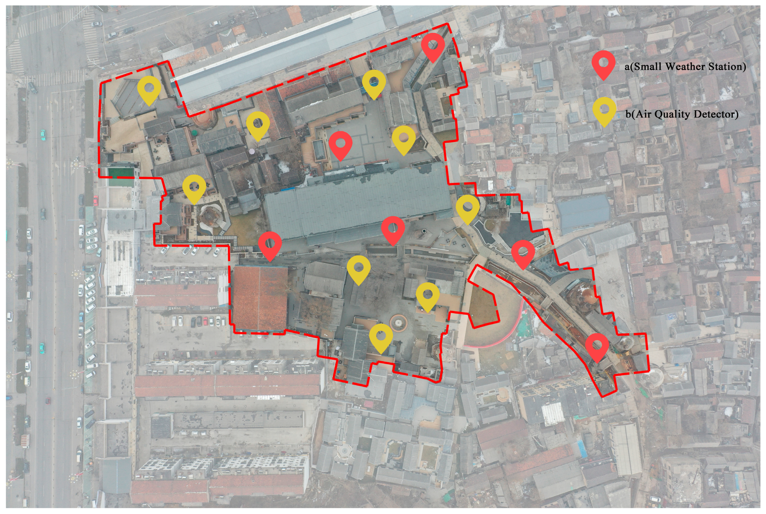
In order to ensure that the monitor points will not be directly affected by the pottery kiln chimney pollution sources and to ensure the accuracy and reliability of the data, the monitor points were arranged to cover the entire block as much as possible and to be able to cover the characteristics of the different spatial type of the block. The principle was to take the pollution source as the origin for the sequential distribution of points. The weather station was fixed 2 m away from the ground to accurately collect the nearby particulate matter and reduce the impact (damage) of human factors on the weather station. Meanwhile, the hand-held aerosol particulate matter detectors were added in the relevant areas as a data supplement (Figure 4).
Field monitoring was conducted continuously for six days from 12–18 October 2021, and the monitoring time lasted from 9:00 to 17:00 every day, which was the peak period of production in the pottery kiln and the time period when PM2.5 particulate matter was continuously produced, so the time period was typically representative. Samples were continuously collected in the small weather station, and particle concentration data were extracted from different areas simultaneously on the same day. The hand-held aerosol particulate matter detector collected data simultaneously on different green space structures. Different hand-held devices were used to detect for one minute at collection points simultaneously. The detection was conducted nine times at different green space structure sites simultaneously.

3.2.2. Comparison of Field Detection and Fluent Model Simulation

According to the data obtained from the weather station monitoring points, four modeling areas with different block types were constructed: D1, D2, D3, and D4, which were monitor points in the green space of the block. Each model area in the block was 70 m × 40 m with a vertical height of 50 m. The size of grid cells was set to be 0.5 m × 0.5 m × 0.5 m. Plant species the model did not cover were replaced with the closest plant species, and parameters such as tree heights and LAI were entered. The day with the lowest air pollution fluctuation among the six days of testing was chosen as P5. The model simulation was carried out under typical weather (no rain and wind speed below 3 m/s) with pollution fluctuation levels of P1, P2, P3, P4, P5, and P6 (six pollution levels according to the national air quality classification standard for AQI) (Table 5).
By verifying the wind speed values and PM2.5 values from the field monitoring and Fluent model simulation (Table 6), the linear regression line shows that the simulation study of the Fluent model has adaptability and accuracy that meet the study requirements of PM2.5 particulate matter concentration in the block (see Figure 5).

4. Results and Discussion

4.1. Characteristics of the Distribution of PM2.5 Concentration in Different Block Angle Types in the Prevailing Wind Direction

Under the prevailing wind all year round, the dominant wind direction and the orientation of the blocks produce a corresponding angle, which can affect the distribution of different concentrations of particulate matter on the windward and leeward sides of the blocks. There has been a lot of progress in the study of the influence of the angle between prevailing wind direction and the orientation of streets on the distribution of PM2.5 concentration. Buccolieri et al. [38] showed that the average concentration at trees increased to 108% under the condition that the prevailing wind direction was perpendicular to the orientation of streets and that the average concentration in the pedestrian area decreased by 18% under the condition that the prevailing wind direction was horizontal to the orientation of streets. Amorim et al. [39] performed air quality simulations using two CFD models and found that the CO concentration increased by 12% when the prevailing wind direction was 45° to the orientation of streets, and the CO concentration decreased by 16% on average when the prevailing wind direction was almost parallel to the orientation of streets. Gromke et al. [40] focused on the impact of street trees on pollutants under the condition that the prevailing wind direction was 45° to the orientation of streets. Vranckx et al. [41] showed that the pollutant concentration on both sides of the street valley increased when the incoming wind direction was 45° and horizontal, which was consistent with the previous wind tunnel test results. Therefore, based on the existing research results, two key angles of 45° and 90° were selected to stimulate the influence of the prevailing wind direction and the orientation of streets on PM2.5 concentrations in summer and winter in rural areas through CFD steady-state simulation, as shown in Figure 6 and Figure 7.

4.1.1. Characteristics of the PM2.5 Concentration Distribution of the 45° Angle of the Street in the Prevailing Wind Direction

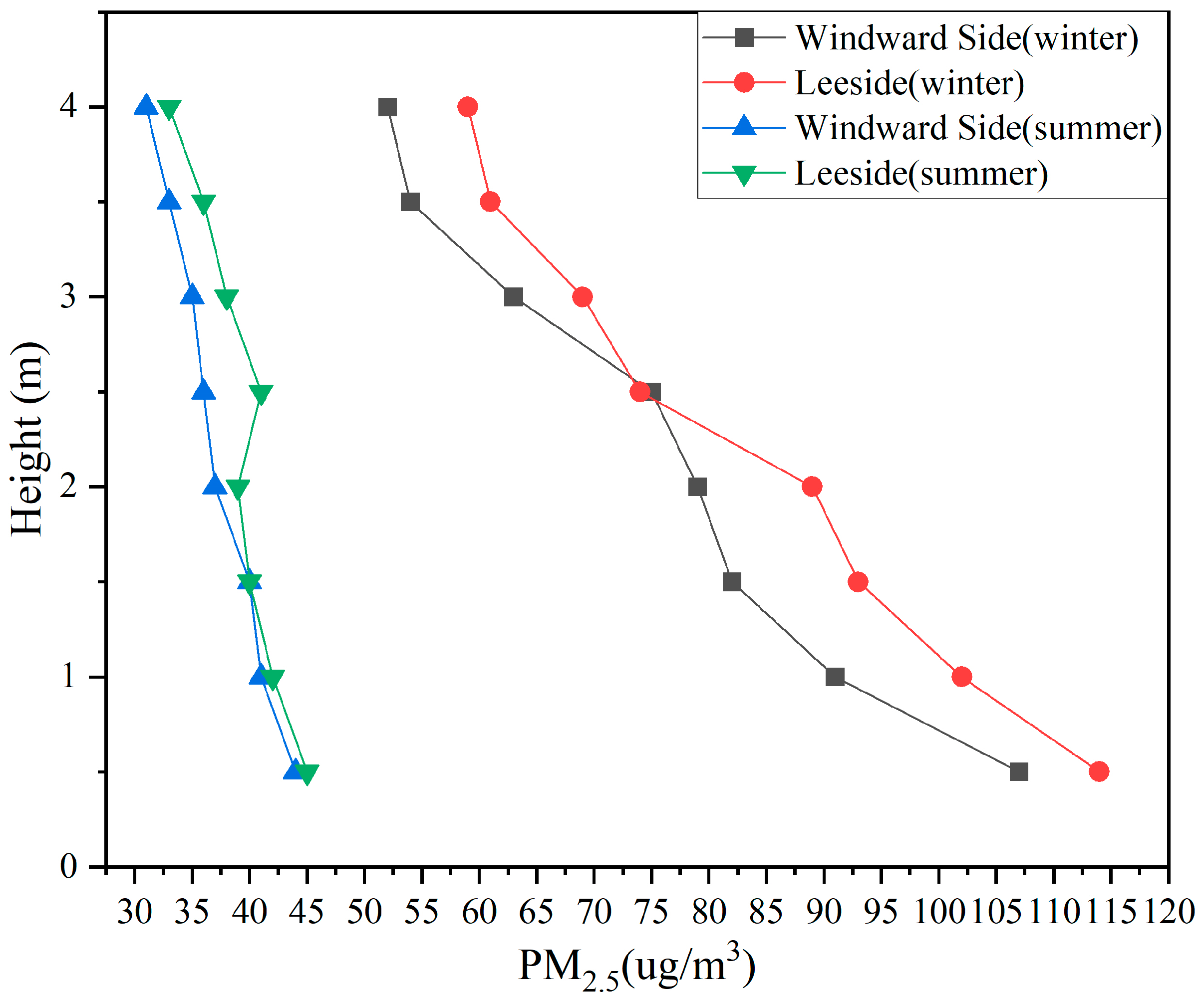
In the 45° angle of the street in the prevailing wind direction and for the 45° incoming wind presents, there are windward and leeward sides of the block in summer and winter. The pollutant concentrations on both sides of the wall within the street valley increased. Figure 8 shows a relative difference between the windward and leeward sides of the block and in the prevailing wind direction. In particular, the PM2.5 particulate matter concentrations reached the highest on the leeward side in winter, and the PM2.5 particulate matter concentrations reached the lowest on the windward side in summer, which varies significantly with increasing height on both sides of the block. The highest PM2.5 particulate matter concentration occurs in the range of 0–1.5 m. The fluctuation is relatively mild in the range of 1.5–2.5 m, and the PM2.5 particulate matter concentration decreases significantly in the range of 2.5–4.0 m. The overall trend is decreasing.

4.1.2. Characteristics of the PM2.5 Concentration Distribution of the 90° Angle of the Street in the Prevailing Wind Direction

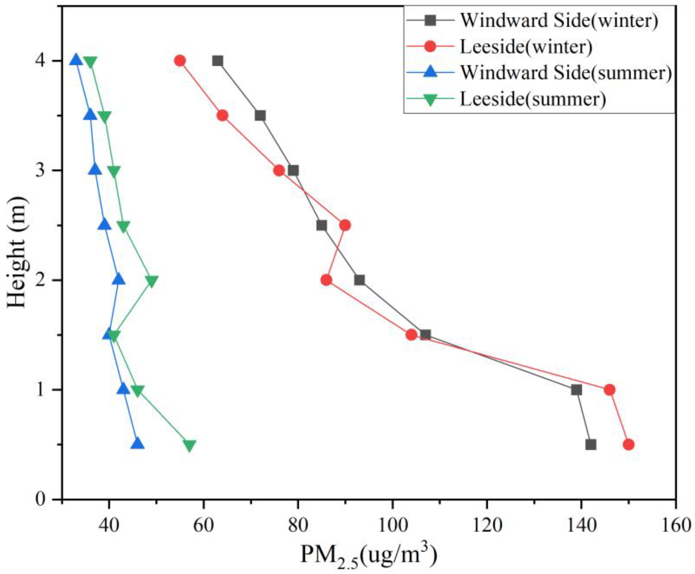
At the 90° angle of the street in the prevailing wind direction, the pollutant concentrations of PM2.5 particulate matter on both sides of the wall within the block show an order of magnitude increase relative to the 45° angle wind direction. Figure 9 shows a significant difference between the particulate matter concentrations on the windward and leeward wall spaces in the block in the prevailing wind direction. The highest PM2.5 particulate matter concentration on the leeward side in winter reaches 150 ug/m3, and it changes significantly with the increase of height on both sides of the block.

4.2. Analysis of Characteristics of the PM2.5 Concentration Distribution of Different Vegetation Types in Streets

At a local level, the ability of vegetation to capture PM is more complicated to define, involving dispersion, including sedimentation processes under gravity, diffusion, and turbulent transfer. The porous structure of trees can alter airflow and increase air turbulence and vertical mixing, which contributes to the dispersion and uptake of PM [42]. There are different types of vegetation in the streets. According to the field research, there are mainly three types of vegetation in Zibo city: trees, shrubs, and grass. The three types of vegetation include enclosed, incremental, and centralized types. Trees are mainly deciduous broadleaf trees. Shrubs are mainly holly and grassland. The specific vegetation type is shown in configuration in Table 5. The deciduous broad-leaved tree communities are neat in appearance, with straight trunks and a rich understory of shrubs and herbs [43,44,45,46]. The trees are full of leaves. The forest canopy is lush, and the foliage index is relatively large, which has a good deposition effect on PM2.5 and PM10 particulate matter. Limited by the canopy size, deciduous broadleaf trees are mainly distributed in main streets with large spaces. Deciduous shrubs and small trees are the main vegetation types in the street due to the limited space. Therefore, the proportional relationship between the spatial dimensions of different combinations of vegetation types and the size of the vegetation canopy also directly affects the concentration of pollutants in streets and the dispersion efficiency.
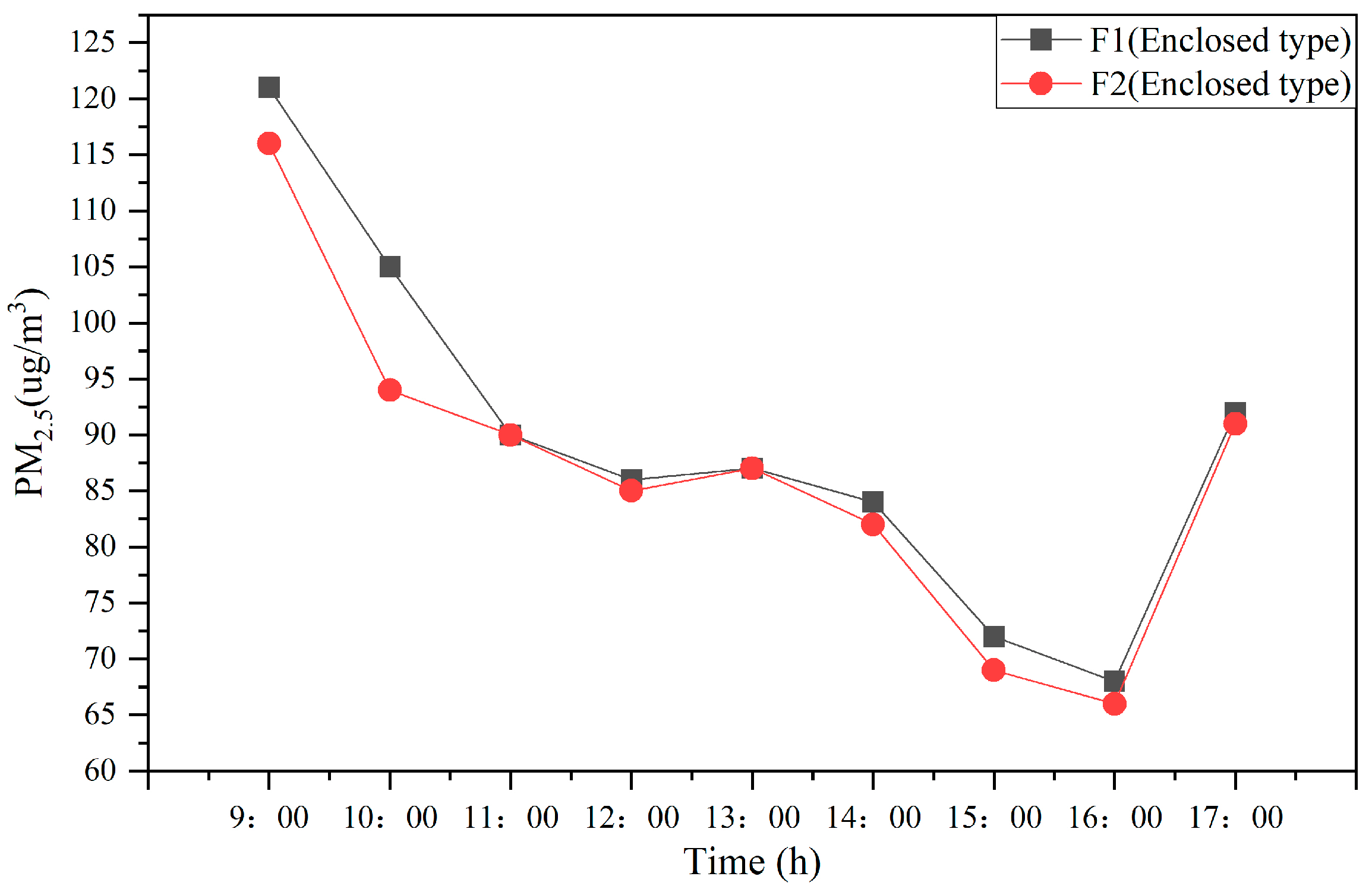
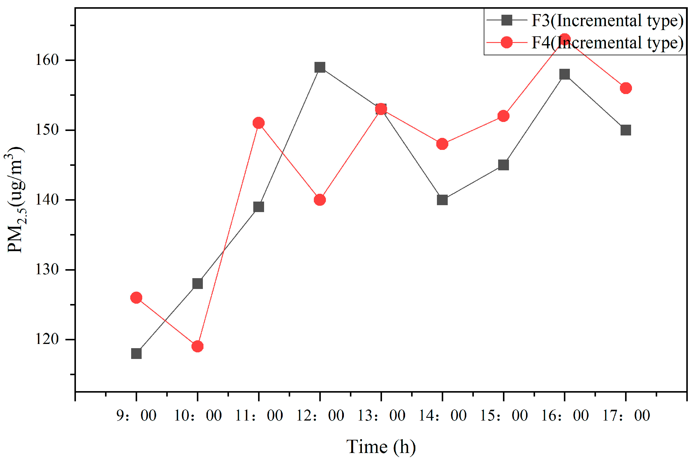
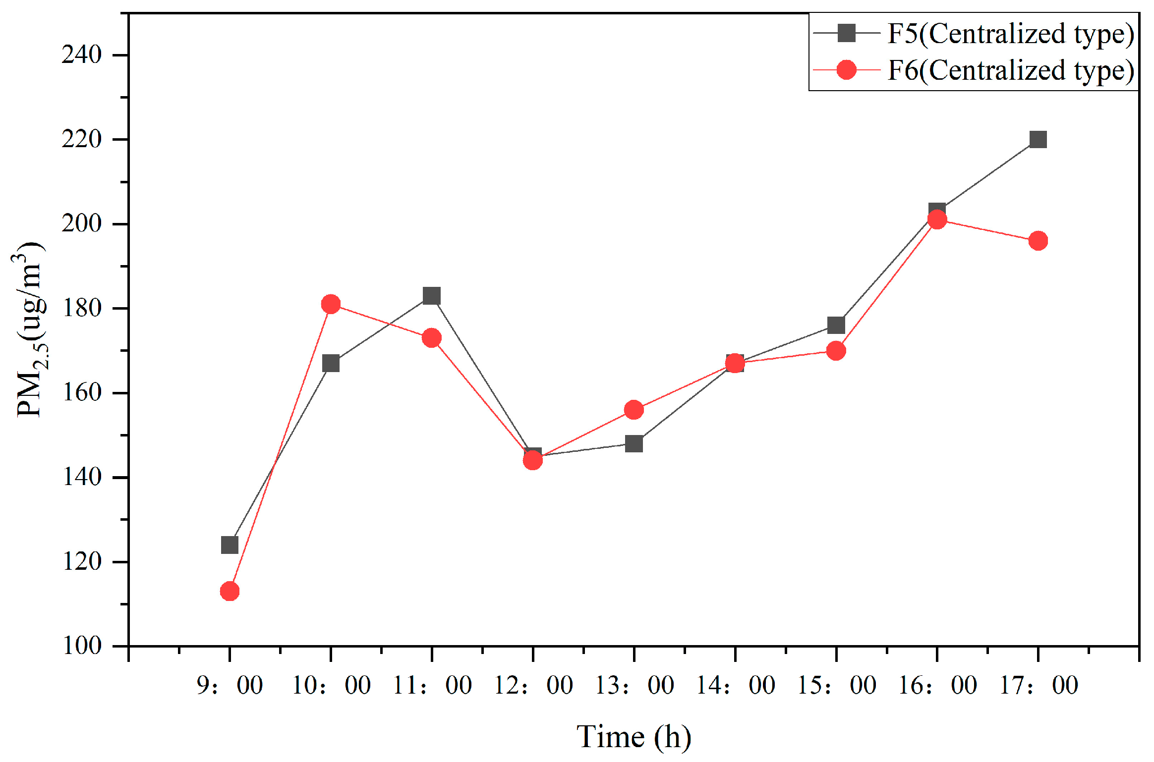
Through the transient simulation test of different vegetation types lasting for 9 h, the diurnal variation of atmospheric PM2.5 concentrations at the flow field cross-section of Z = 1.5 m was revealed under the same pollution level, of 120 ug/m3. It was found that the green space structures with different vegetation types significantly influenced the diurnal variation of atmospheric PM2.5 concentrations. Under the same pollution conditions, the PM2.5 concentration in the green space structures of the enclosed vegetation type (F1–F2) shows a decreasing trend overall and lasts for a relatively long time, reaching the lowest value at 4:00 p.m. and increasing accordingly with the increase of time thereafter (Figure 10). In the green space structure of the incremental vegetation type (F3–F4), the PM2.5 concentration shows an overall slow rising trend and continues to fluctuate (Figure 11). The unilateral absorption surface of the incremental vegetation type leads to a general absorption effect on PM2.5 particulate matter. The concentration reaches the lowest value at 10:00 a.m., showing a fluctuating increase thereafter. In the green space structure of the central vegetation type (F5–F6), the PM2.5 concentration shows an overall increasing trend, with a rapidly rising trend at the beginning (Figure 12). However, the subsequently sustained capacity is insufficient. When the particulate matter keeps settling in the trees and then shows a decreasing trend, the PM2.5 concentration increases after 12:00 p.m.

4.3. Impact of Different Distances between Vegetation and Buildings in the Block on the PM2.5 Concentration Distribution

A strong reduction in the mean flow and turbulence intensity can be observed within the canyon due to the increase in the LAI. The air exchange rate AER = ∫Γ(w + |roof +1/2ww’|roof)dΓ at the roof level is usually employed to represent the rate of removal of airflow in street canyons [47,48].
Different distances between vegetation species and buildings in the neighborhood have significant effects on the PM2.5 particulate matter concentration distribution in the block. The plant canopy is used as the source point, and two main types of trees and shrubs were selected from distances of 1 m, 2 m, and 3 m from the buildings on the same side (Table 7). The plants in the block have 50% canopy density, forming six related types. The change of the atmospheric PM2.5 concentrations at the flow field cross-section of Z = 1.5 m was measured using a CFD steady-state simulation test with 120 ug/m3 as the input pollution level.
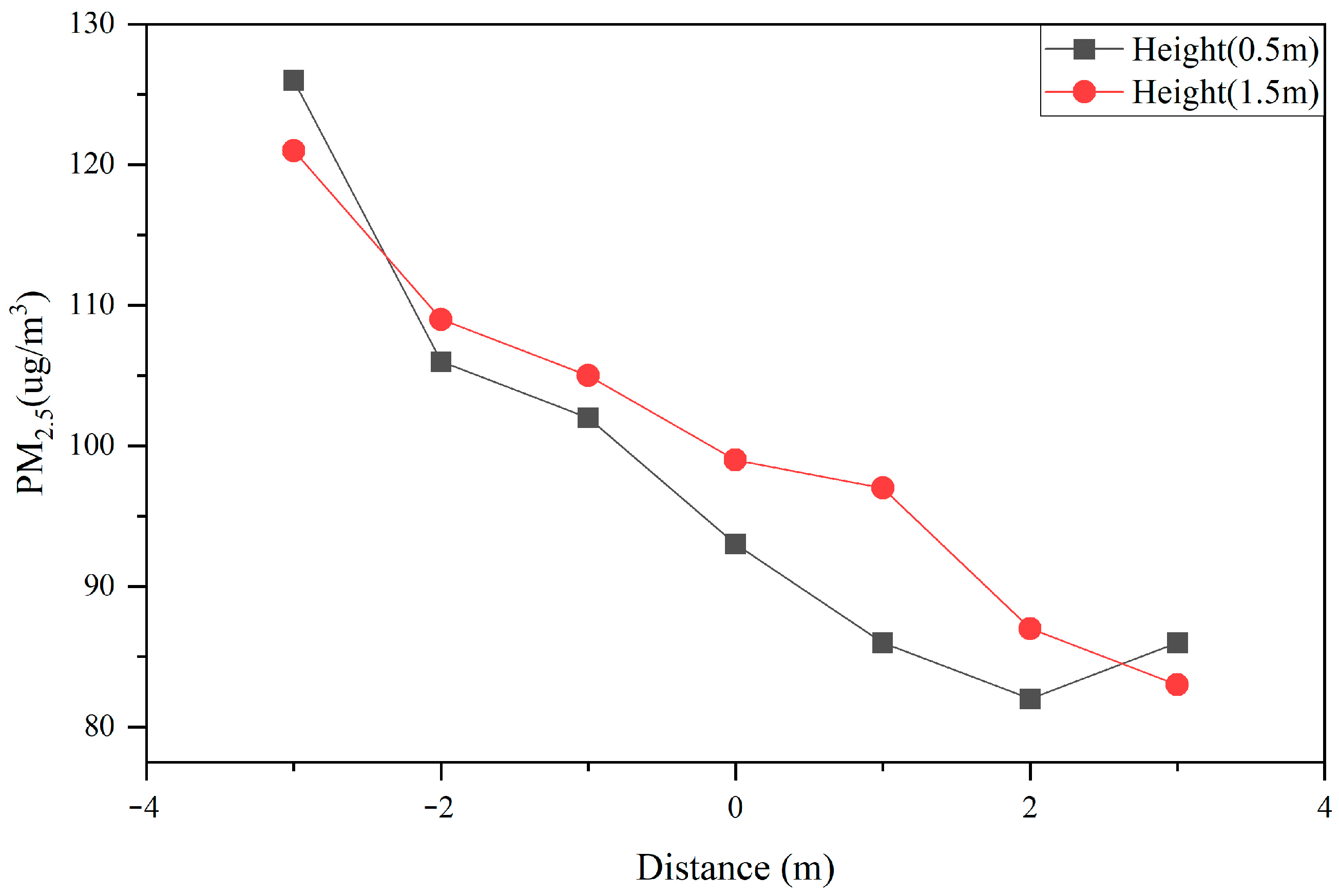
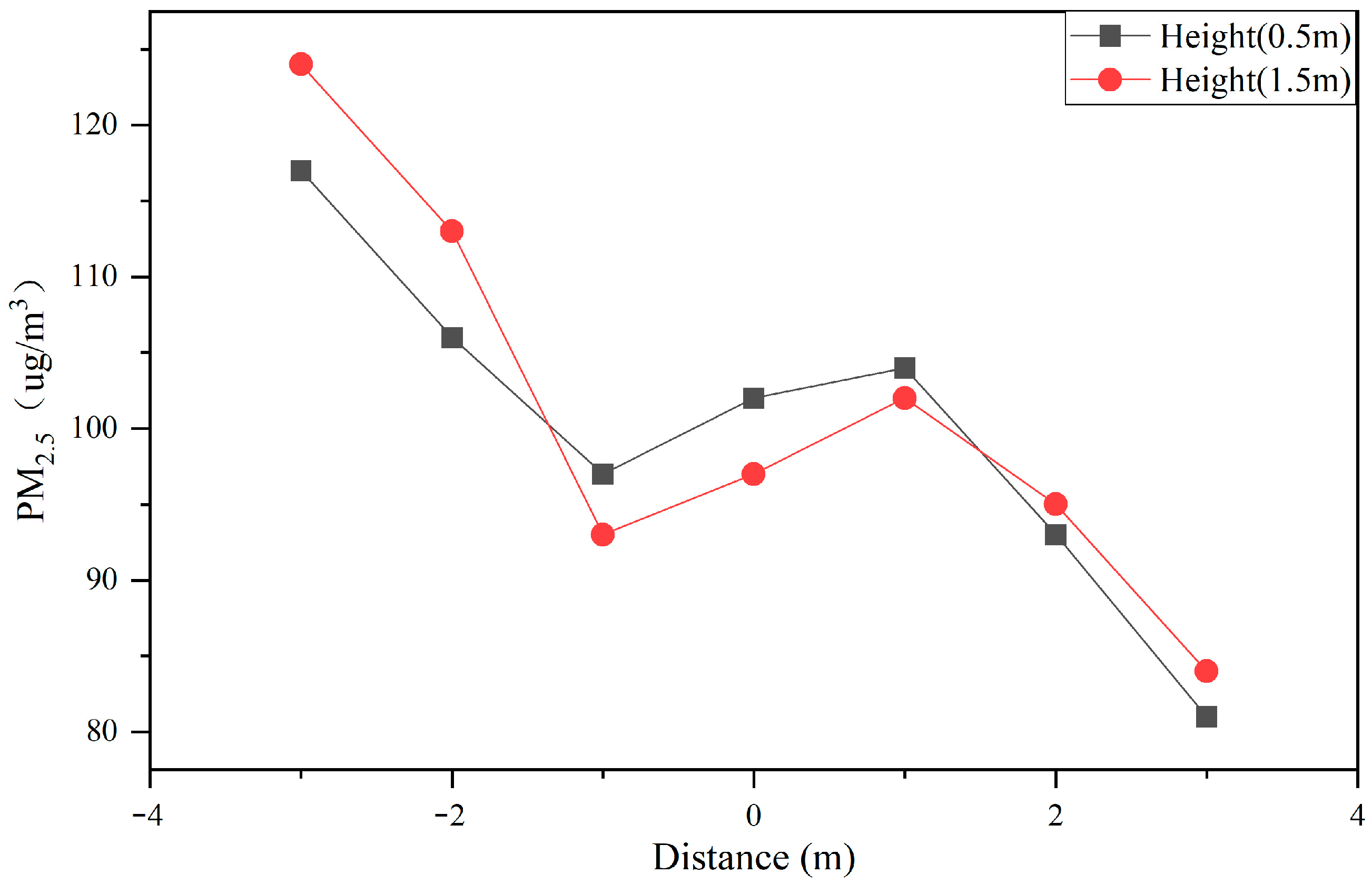
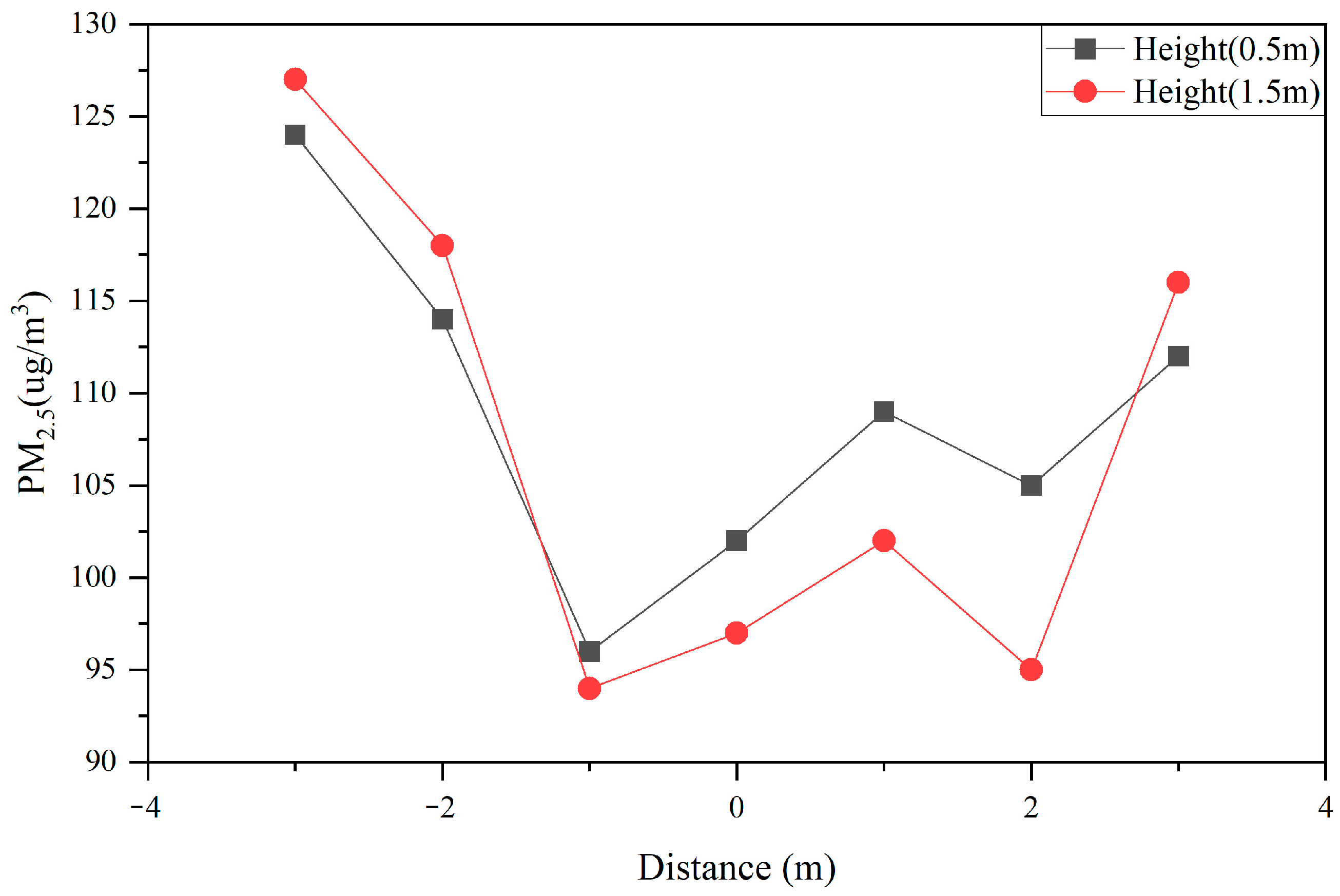
When the tree plants are 1 m away from the building on the same side, the PM2.5 particulate matter concentration in this range is the lowest, with the lowest value reaching 82 ug/m3. The accumulation of PM2.5 particulate matter appears under the plant canopy in a few areas. When the trees and plants are 2 m away from the same side of the building, the PM2.5 particulate matter in this range has a corresponding increase leading to an increase in the concentration. The overall PM2.5 particulate matter concentration in the block maintains a decreasing trend. When the trees and plants are 3 m away from the buildings on the same side, the PM2.5 particulate matter concentration in the area shows a significant rising trend and reaches the highest value of 116 ug/m3 within the range of human activities. It is shown in Figure 13, Figure 14 and Figure 15.
Simulations related to six types of distances between vegetation and buildings in the block show that the canopy size of trees influences the results at a distance of 1 m. Because the inner side is against the wall, the dust retention effect of PM2.5 particulate matter on the outer and inner sides gradually converges with increasing distance. The overall dust retention effect of PM2.5 particulate matter of shrubs tends to level off with increasing size between shrubs and buildings. There is no curve fluctuation of the dust retention effect of trees. Regardless of the distance, the tree canopy prolongs the movement and retention time of suspended PM2.5 particulate matter around the trees, resulting in the aggregation of particulate matter in the tree leaves and making the PM2.5 particulate matter concentrations around the trees significantly lower than those around the shrubs. Moreover, the tree canopy intercepts suspended particulate matter in the downward airflow in the vortex, resulting in lower particulate matter concentrations within the human activity area.

4.4. Variation and Analysis of the Effect of Vegetation Height and Different Heights of Buildings on Both Sides on PM2.5 Concentration

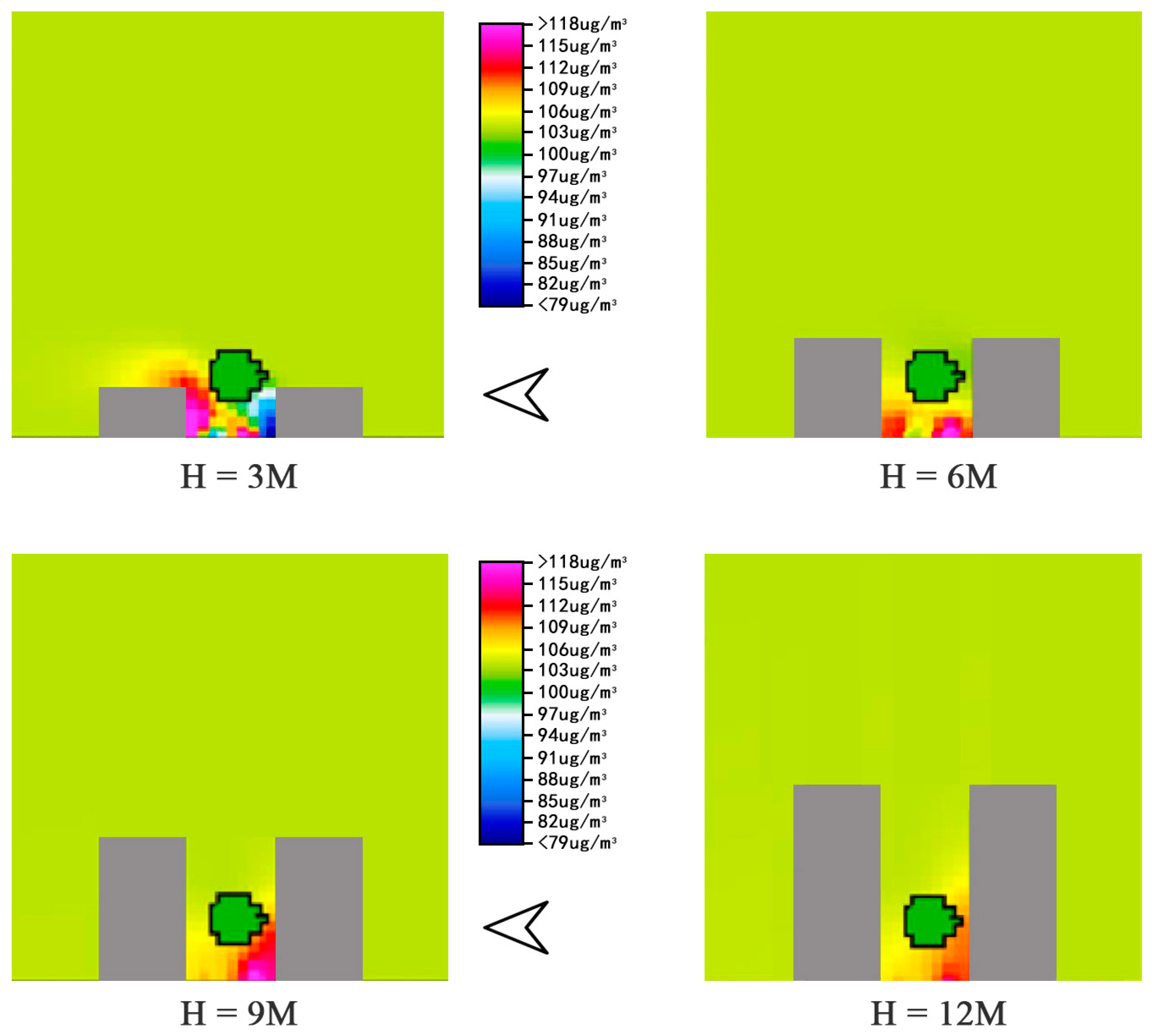
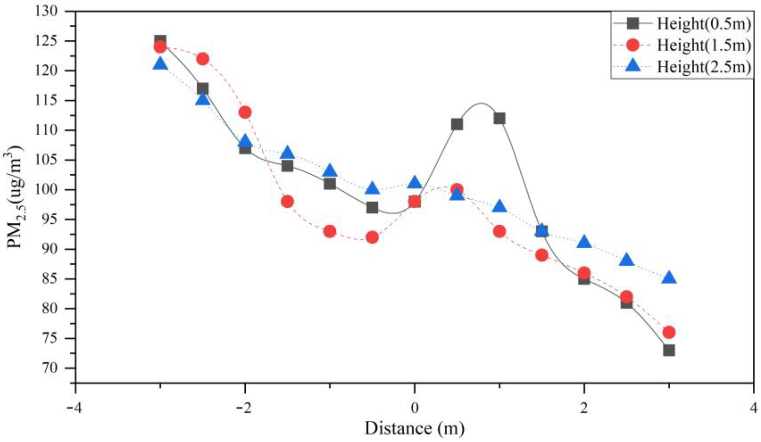
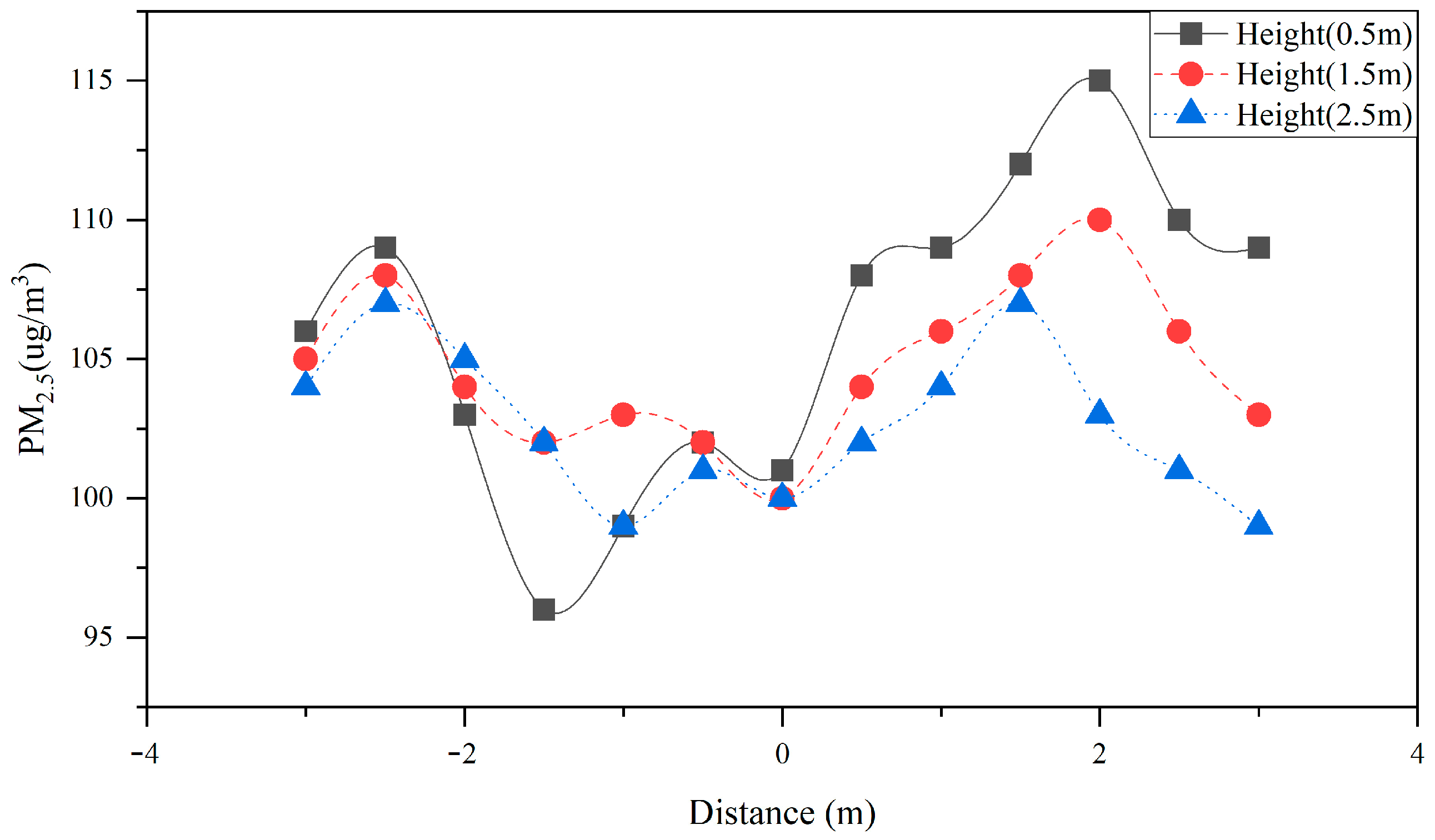
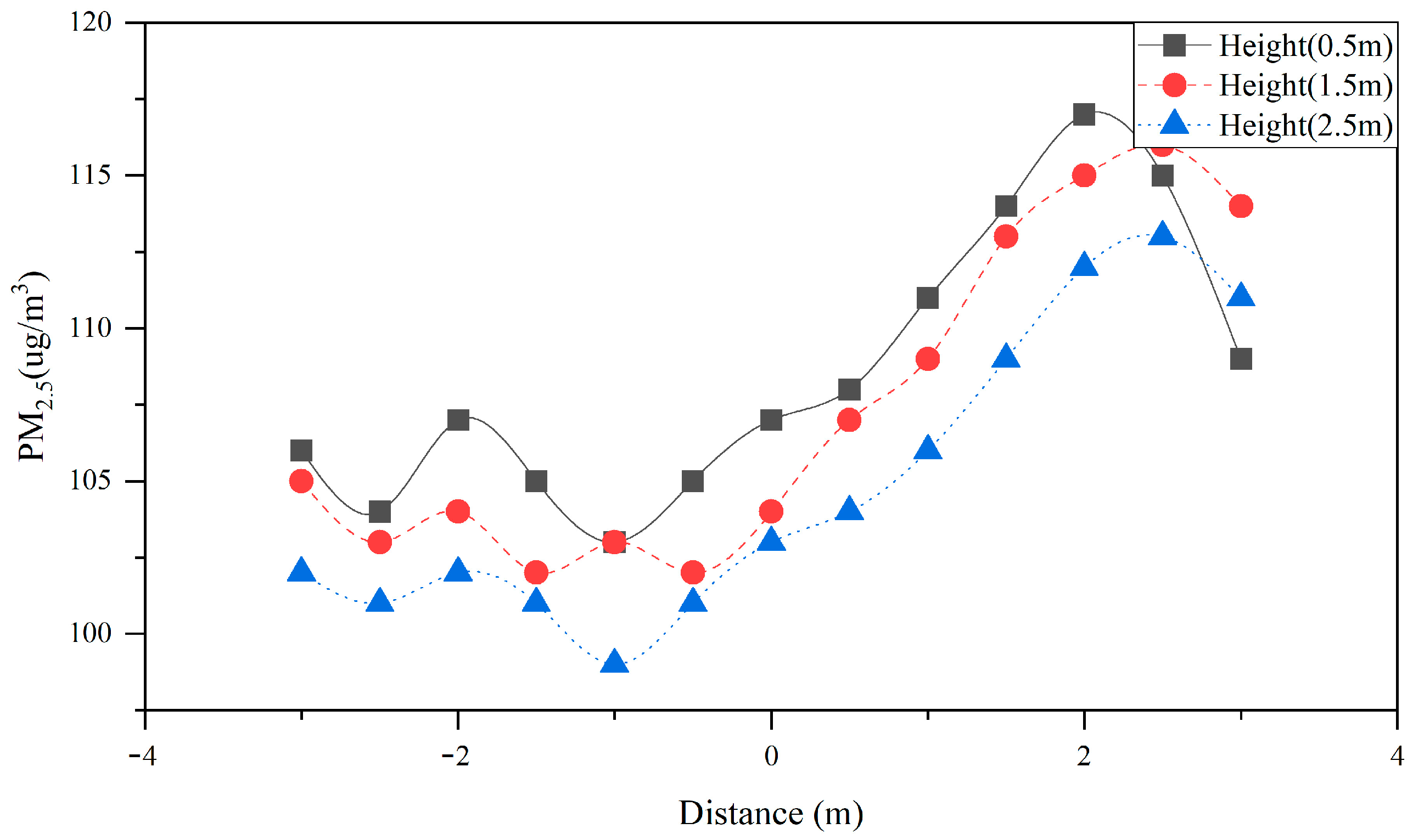
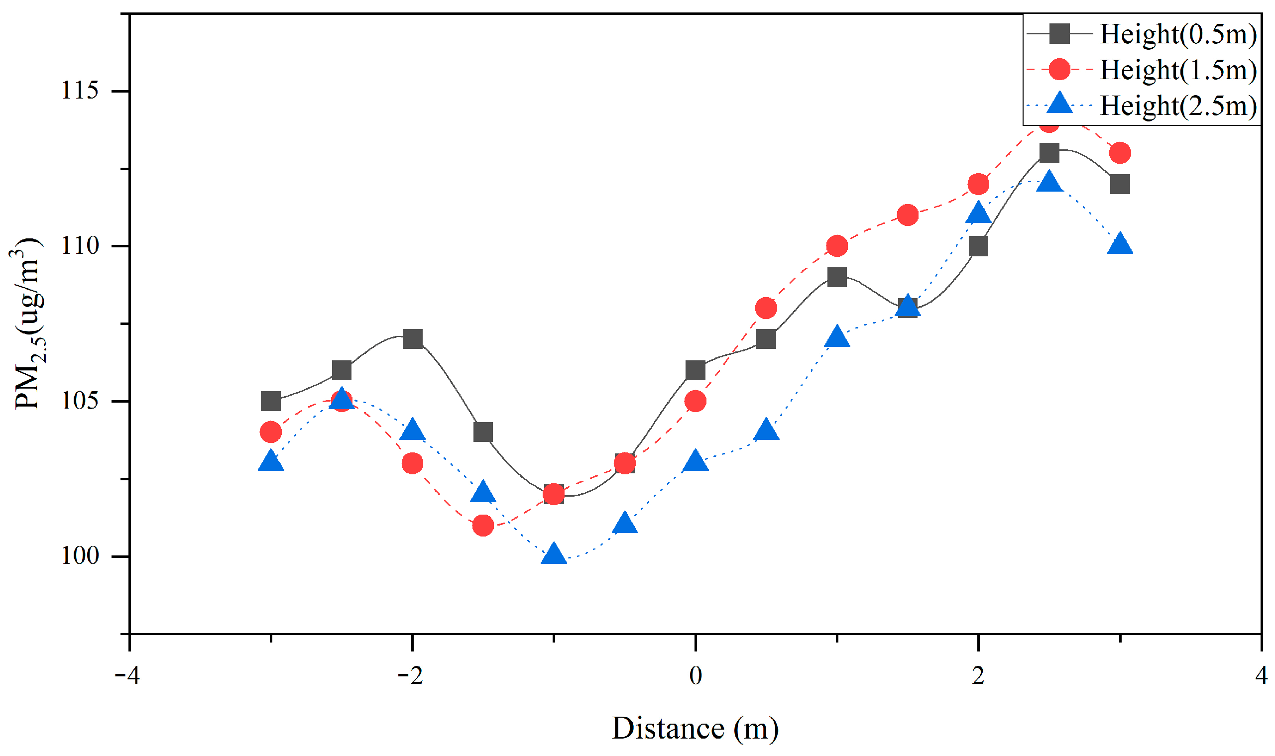
There were many studies on the factors of pollutant dispersion in street canyons, such as environmental wind direction (Vranckx et al. [41]), plant influence (Li et al. [49]), and building layout and configuration, including building height (Nosek et al. [50]), roof geometry (Llaguno et al. [51]), etc. In rural streets, the roof geometry is relatively consistent, and there are differences in the heights of buildings on both sides of the street. When the angle between the prevailing wind direction and the block was 90°, the orientation of the blocks had a relatively stable effect on the PM2.5 concentrations at the height of the vegetation in the block and the height of the buildings on both sides of the street, so it became a simulated environment with different heights of vegetation and buildings on both sides [52]. When the height of the plants in the blocks was 5 m, and the heights of the buildings on both sides were 3 m, 6 m, 9 m, and 12 m, respectively, the change of atmospheric PM2.5 concentrations at the flow field cross-section of Z = 1.5 m was tested using CFD steady-state simulation, with 120 ug/m3 as the input pollution level. With the increase of the building height on both sides of the block, the PM2.5 concentration distribution around the plants changed significantly. Meanwhile, there were significant differences in PM2.5 concentration distribution between the windward and leeward sides of plants.
When the building height on both sides of the block plants is 3 m, the concentration of PM2.5 particles on the windward side of the plants is the lowest. The lowest PM2.5 concentration is found at the bottom of the building. There is a negative correlation between PM2.5 concentrations and the increased building height. The PM2.5 concentration between the leeward side of the plant and the buildings decreases with increasing height. The highest value of particulate matter concentration is at the very bottom of the building, where the accumulation of particulate matter is serious because it is sheltered from the plants of this height.
When the height of the buildings on both sides of the neighborhood plants is 6 m, the PM2.5 particulate matter concentration area shows an up-and-down distribution. The highest particulate matter concentration area is concentrated at the roots of the plants and the bottom of the buildings. The lowest PM2.5 concentration value of the plants occurs at the canopy, while the PM2.5 particulate matter concentration at the roots of the windward side of the plants is higher than that at the leeward side as a whole.
When the building height on both sides of the plants in the block is 9 m, PM2.5 particulate matter is mainly concentrated on the windward side of the plants. The area with the highest concentration is at the bottom of the building. The area with the highest concentration is at the bottom of the building. The leeward side of the plant is less affected, and the lowest concentration is at the bottom of the building on the windward side of the plant. When the building height on both sides of the block plant is 12 m, the accumulation of PM2.5 particulate matter is similar to the distribution characteristics at 9 m. However, the highest concentration value is lower, and the higher the building height on both sides, the more obvious the decreasing effect is. It is shown in Figure 16, Figure 17, Figure 18, Figure 19 and Figure 20.
The height of different vegetation and the different heights of buildings on both sides form different horizontal and vertical ratios, which is AR = H/W. Four different horizontal and vertical ratios of vegetation and building heights on both sides were set in the model. The plant height of deciduous trees with 50% canopy density in the block and buildings with a height of 3 m from the control group; the building heights on both sides were 3 m, 6 m, 9 m, and 12 m.
With the increase of H/W, the overall PM2.5 particulate matter concentration in the block decreases at first and then increases. The minimum PM2.5 particulate matter concentration difference gradually increases from negative values. Meanwhile, the distribution of the PM2.5 particle concentration field in the block is influenced by H/W. In the range of H/W = 0.5–2, PM2.5 particle concentration is the lowest in the block. The minimum concentration difference is −3.11 ug/m3, and the minimum concentration is 4.081 ug/m3. In the range of H/W = 3–4, the PM2.5 particulate matter concentration in the block is relatively high, the minimum concentration difference is 0 ug/m3, and the minimum concentration is 36.6 ug/m3.

4.5. Impact of Different Street Tree Configurations on the PM2.5 Concentration Distribution in the Block

Generally, when air carrying PM passes through the community canopy, large-sized particles are more likely to be intercepted and deposited on the surfaces of branches, leaves, and stems [53]. In contrast, Liu et al. [54] found that PM2.5 level was positively correlated with CD, LAI, and average tree diameter but negatively correlated with average tree height, forest land area, herbaceous coverage, and height. Furthermore, a study has shown that leaf area and tree canopy increased transpiration and the interception of solar radiation, which can cool the air beneath trees and form cool islands around trees [55]. The PM2.5 consumption rate in the front part of the green space was higher than that in the middle or rear part. One potential reason for this result may be that tall trees in front of the green space greatly slow down the wind speed, which promotes the deposition of PM2.5 and reduces the dispersion of PM2.5 [56].
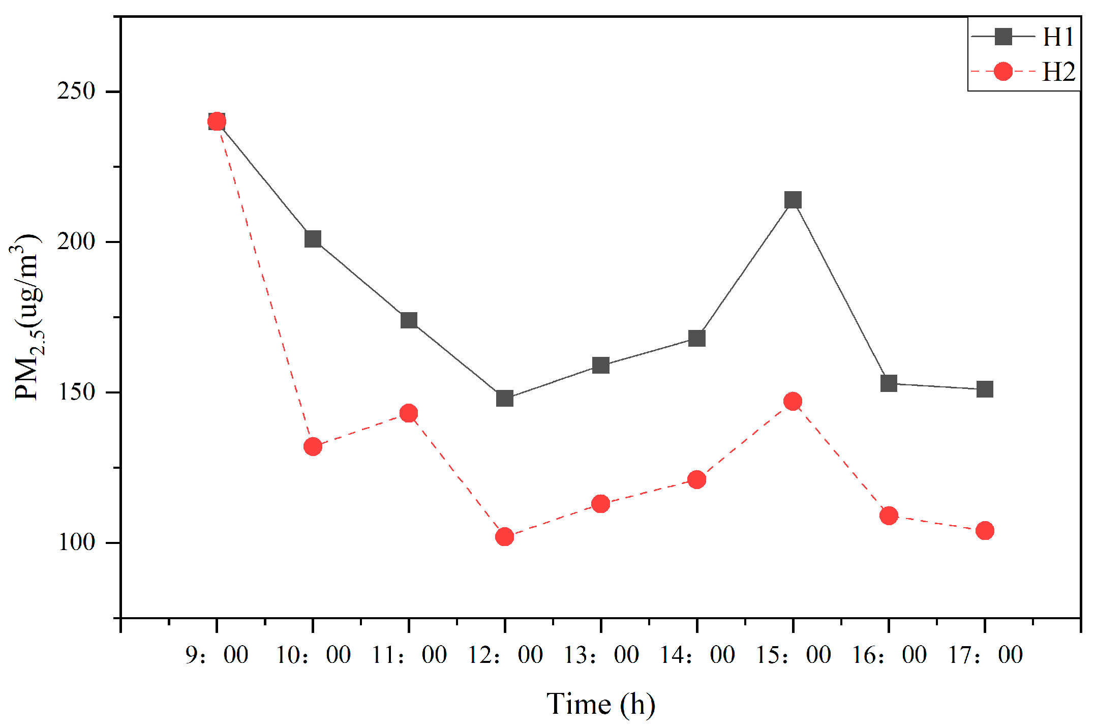
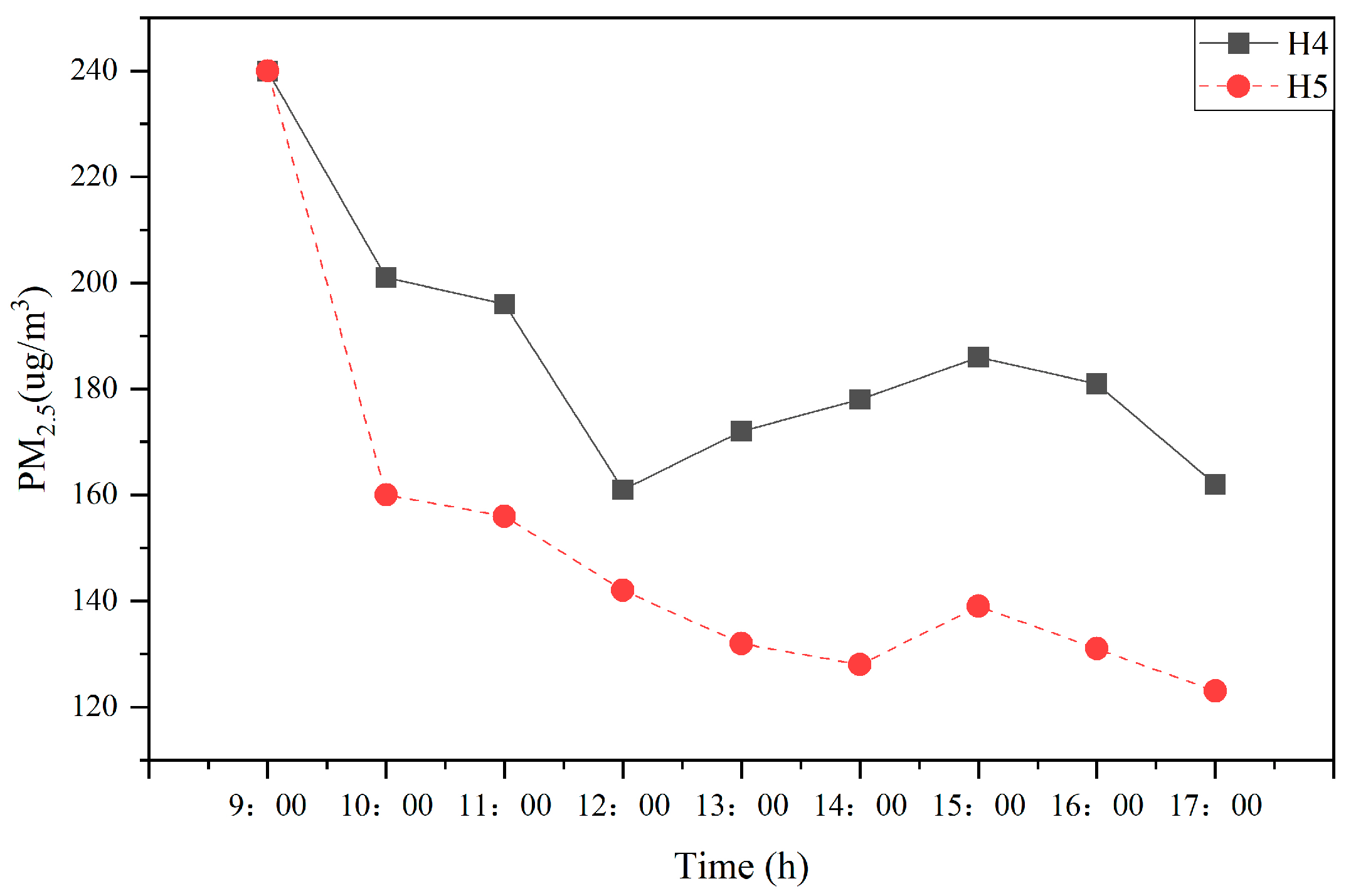
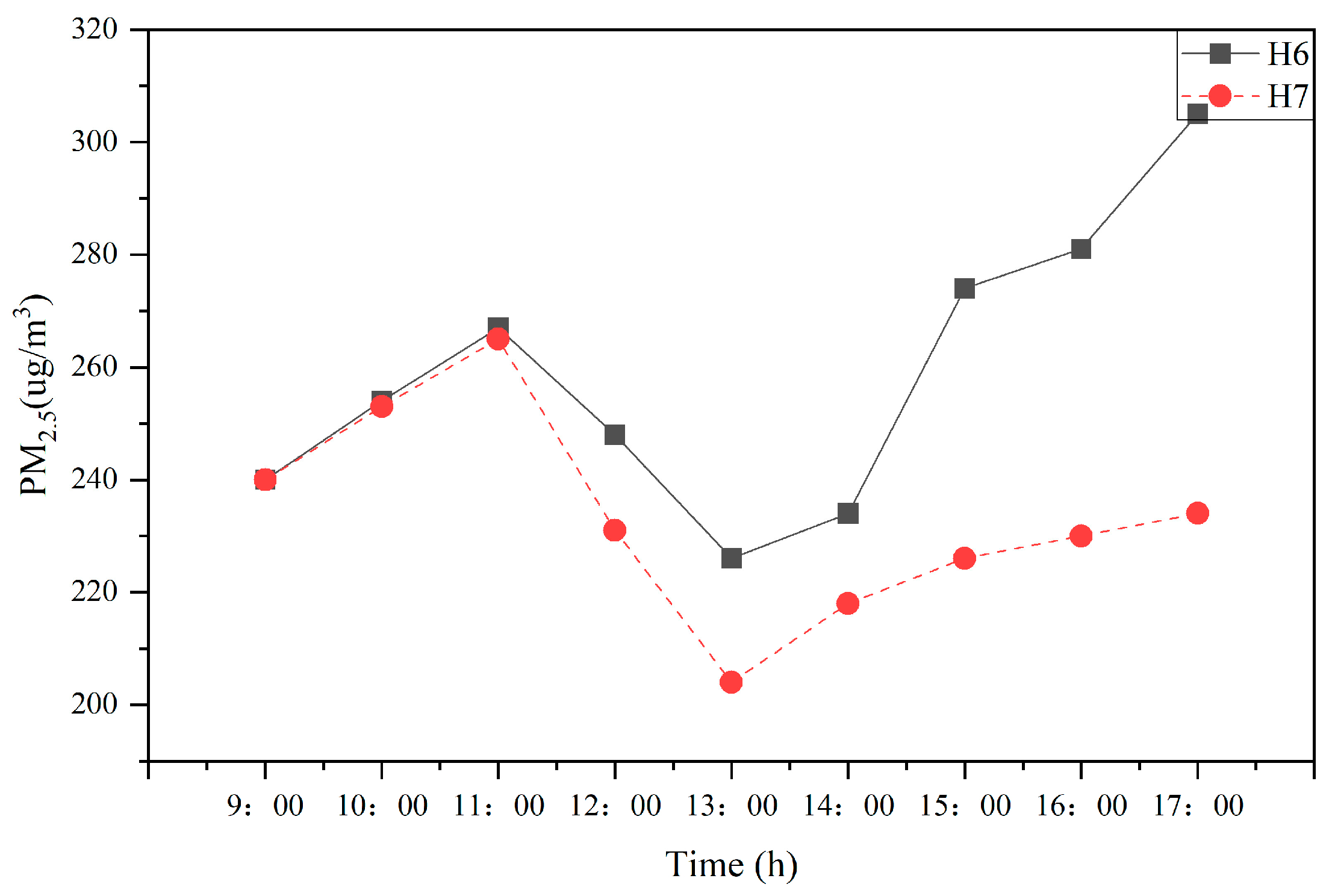
Through the transient simulation test of eight kinds (H1–H8) of different street tree configurations lasting for 9 h, the diurnal variation of atmospheric PM2.5 concentrations at the flow field cross-section of Z = 1.5 m was revealed under the same pollution level of 200 ug/m3. It was found that different street tree configurations had different effects on PM2.5 concentrations. The street tree configuration of H5 within the range of human activities at the cross-section of Z = 1.5 m had the best effect in reducing PM2.5 concentrations, as shown in Figure 21, Figure 22, Figure 23 and Figure 24.
The influence of eight (H1–H8) street tree configurations in the block on the PM2.5 particulate matter concentrations was studied. The same XZ section data were selected and made into a table. The results showed that different street tree configurations had different effects on PM2.5 particulate matter concentrations, and the street tree configuration of H5 within the range of human activities had the best effect on reducing PM2.5 particulate matter concentrations, as shown in Figure 21, Figure 22, Figure 23 and Figure 24.
The PM2.5 concentration of H1 and H2 structures decreases from the middle to the outside, and they have a better purifying effect on PM2.5. The concentration difference in PM2.5 particulate matter between H4 and H5 shows an elongated concentric ellipse. The area in front of the green space has no purifying effect on PM2.5. As moving toward the center of the green space, the purification area of H4 and H5 on PM2.5 particulate matter concentration gradually expands, while the purification ability of the street tree configuration of H5 is better than that of the street tree configuration of H4. PM2.5 particulate matter concentration between H6 and H7 has a good reduction effect on PM2.5 particulate matter in most front and back areas, but PM2.5 particulate matter concentration is higher in the middle area, and this effect is more obvious with the increase in height. PM2.5 particulate matter concentration between H3 and H8 has a good decreasing effect within the human activity range during a short time. However, as the time and height increase, PM2.5 particulate matter concentration also increases successively, leading to the aggravation of the concentration within the human activity range.

5. Conclusions

On-site monitoring and CFD simulation of the prevailing wind directions, block space structures, and green space plant configurations in industrial-production-oriented villages showed that different structures and spatial locations of green space had significant differences in atmospheric PM2.5 concentrations. At the same time, CFD simulations can well describe the differences in the distribution of atmospheric PM2.5 concentrations in different green space structures and the impact of green space on atmospheric PM2.5 concentrations. Field monitoring of the prevailing wind direction, the spatial structure of existing neighborhoods in the countryside, and the configuration structure of green space plants showed that PM2.5 concentrations differed significantly among different green space structures and spatial locations and that green space structure had a significant effect on the daily variation of atmospheric PM2.5. Although the simulated values of the Fluent model differed from the actual measured values, the CFD simulations well depicted the differences in the distribution of atmospheric PM2.5 concentrations in different green space structures and the influence of green space on atmospheric PM2.5 concentrations.
In general, the influence of different angles between the prevailing wind directions throughout the year (the dominant wind directions are northeast (NE) and south–southwest (SSW) in summer and winter, respectively), and the orientation of blocks on the distribution of PM2.5 concentrations was significantly different. With the included angle, the average PM2.5 concentration on the windward side was 9.4 ug/m3 lower than on the leeward side. The highest PM2.5 concentration occurred in the interval of 0–1.5 m, and the fluctuation was relatively gentle in the interval of 1.5–2.5 m, while the concentration decreased significantly in the interval of 2.5–4.0 m. In winter, when the included angle was 90°, the PM2.5 concentration on the leeward side of the block reached a maximum of 150 ug/m3. Linear regression analysis showed R2 = 0.5117 for the enclosed green space structure, R2 = 0.4804 for the centralized green space structure, and R2 = 0.6875 for the incremental green space structure, and the enclosed green space structure showed a downward trend during the day. When the arbor plants were 1 m away from the building on the same side, the PM2.5 concentration within this range was the lowest, with the lowest value of 82 ug/m3, and there was a small area of PM2.5 accumulation under the plant canopy. When the vegetation was higher than the building, PM2.5 was distributed on the leeward side. When vegetation height was equal to buildings on both sides, the PM2.5 distribution on the windward and leeward sides tended to be equal. When vegetation height was shorter than buildings on both sides, the PM2.5 concentration on the windward side was higher than on the leeward side. The distribution of PM2.5 concentrations was significantly affected by different street tree configurations in the block, among which the concave (H5) street tree configuration reduced the PM2.5 concentration by 39%, and the uniform (H1, H2, H3, H8) street tree configuration increased the PM2.5 by 20%. Therefore, a comprehensive configuration form was formed as follows: the angle between the prevailing wind direction in the area and the orientation of the streets was controlled within the threshold range of 0–45°, with enclosed or incremental green space structure and concave (H5) street trees, and the height of the vegetation was higher than the height of the buildings on both sides of the streets, providing a comfortable environment within the scope of human activity space. This form of comprehensive configuration has important guiding significance for future block planning and the maximum utilization of green space resources in blocks.
In the future, this research will be extended to rural master planning layouts and the design choices of landscape plants. Based on these data, it can be considered to predict the comfort of different functional spaces with PM2.5 particulate matter in spaces such as productive villages. Future research will focus on combining 3D real-time landscape models with PM2.5 simulations to shorten the time-consuming process of 3D model generation, input, and computation. At the same time, the use of cloud-based services in the future can reduce computing time and results sharing and guide rural landscape design more scientifically.

Author Contributions

F.W.: Conceptualization; Supervision; Review & Editing; Writing—original draft. B.S.: Investigation; Writing—original draft; Software; Visualization. X.Z.: Review & Editing; Project administration; Methodology; X.J.: Funding acquisition; Supervision; Validation; All authors have read and agreed to the published version of the manuscript.

Funding

The research was funded by the National Key Research and Development Program of the 13th Five-Year Plan: Study on the development mode and technical path of village and town construction (No. 2018YFD1100200); 2019 Science and Technology Guidance Project of Housing and Urban-Rural Development of Jiangsu Province: Study on the Construction and Evaluation of Village and Town GI under the Guidance of Ecological Livability (No. 2019ZD001015).

Institutional Review Board Statement

It is not needed to require ethical approval.

Informed Consent Statement

Informed consent was obtained from all subjects involved in the study.

Data Availability Statement

The data used to support the findings of this study are included within the article.

Conflicts of Interest

The authors declare no conflict of interest.

References

  1. Chen, M.; Dai, F. Effects of Urban Green Infrastructure Spatial Pattern on PM2.5 Based on MSPA. Chin. Landsc. Archit. 2020, 36, 63–68. [Google Scholar]
  2. Song, C.; Wu, L.; Xie, Y.; He, J.; Chen, X.; Wang, T.; Lin, Y.; Jin, T.; Wang, A.; Liu, Y.; et al. Air pollution in China: Status and spatiotemporal variations. Environ. Pollut. 2017, 227, 334–347. [Google Scholar] [CrossRef] [PubMed]
  3. Jiang, R.; Hong, B. Spatio-temporal Distribution Characteristics of PM2.5 and PM10 and Residents’ Exposure Risk Assessment in Residential Outdoor Open Spaces. Chin. Landsc. Archit. 2021, 37, 121–126. [Google Scholar]
  4. Dai, F.; Chen, M.; Wang, M.; Zhu, S.; Fu, F. Effect of Urban Block Form on Reducing Particulate Matter: A Case Study of Wuhan. Chin. Landsc. Archit. 2020, 36, 109–114. [Google Scholar]
  5. Razzaq, A.; Sharif, A.; Aziz, N.; Irfan, M.; Jermsittiparsert, K. Asymmetric link between environmental pollution and COVID-19 in the top ten affected states of US: A novel estimations from quantile-on-quantile approach. Environ. Res. 2020, 191, 110189. [Google Scholar] [CrossRef]
  6. Iqbal, W.; Tang, Y.M.; Chau, K.Y.; Irfan, M.; Mohsin, M. Nexus between air pollution and NCOV-2019 in China: Application of negative binomial regression analysis. Process. Saf. Environ. Prot. 2021, 150, 557–565. [Google Scholar] [CrossRef]
  7. Buccolieri, R.; Santiago, J.L.; Rivas, E.; Sanchez, B. Review on urban tree modeling in CFD simulations: Aerodynamic, deposition and thermal effects. Urban For. Urban Green. 2018, 31, 212–220. [Google Scholar] [CrossRef]
  8. Shirzadi, M.; Mirzaei, P.; Tominaga, Y. RANS model calibration using stochastic optimization for accuracy improvement of urban airflow CFD modeling. J. Build. Eng. 2020, 32, 101756. [Google Scholar] [CrossRef]
  9. Piroozmand, P.; Mussetti, G.; Allegrini, J.; Mohammadi, M.H.; Akrami, E.; Carmeliet, J. Coupled CFD framework with mesoscale urban climate model: Application to microscale urban flows with weak synoptic forcing. J. Wind. Eng. Ind. Aerodyn. 2020, 197, 104059. [Google Scholar] [CrossRef]
  10. Santiago, J.L.; Buccoloeri, R.; Rivas, E.; Calvete-Sogo, H.; Sanchez, B.; Martilli, A.; Alonso, R.; Elustondo, D.; Santamaria, J.M.; Martin, F. CFD modeling of vegetation barrier effects on the reduction of traffic-related pollutant concentration in an avenue of Pamplona, Spain. Sustain. Cities Soc. 2019, 48, 101559. [Google Scholar] [CrossRef]
  11. Kadaverugu, R.; Sharma, A.; Matli, C.; Biniwale, R. High-resolution urban air quality modeling by coupling CFD and mesoscale models: A review. Asia-Pac. J. Atmos. Sci. 2019, 55, 539–556. [Google Scholar] [CrossRef]
  12. San José, R.; Pérez, J.L.; Gonzalez-Barras, R.M. Assessment of mesoscale and microscale simulations of a NO2 episode supported by traffic modeling at the microscopic level. Sci. Total Environ. 2021, 752, 141992. [Google Scholar] [CrossRef] [PubMed]
  13. Kim, K.D.; Lee, S.Y.; Kim, J.-J.; Lee, S.H.; Lee, D.G.; Lee, J.B.; Choi, J.Y.; Kim, M.J. Effect of wet deposition on secondary inorganic aerosols using an urban-scale air quality model. Atmosphere 2021, 12, 168. [Google Scholar] [CrossRef]
  14. Park, S.-J.; Choi, W.; Kim, J.-J.; Kim, M.J.; Park, R.J.; Han, K.S.; Kang, G. Effects of building-roof cooling on the flow and dispersion of reactive pollutants in an idealized urban street canyon. Build. Environ. 2016, 109, 175–189. [Google Scholar] [CrossRef]
  15. Rodríguez, M.C.; Dupont-Courtade, L.; Oueslati, W. Air pollution and urban structure linkages: Evidence from European cities. Renew. Sustain. Energy Rev. 2016, 53, 1–9. [Google Scholar] [CrossRef]
  16. McCarty, J.; Kaza, N. Urban form and air quality in the United States. Landsc. Urban Plan. 2015, 139, 168–179. [Google Scholar] [CrossRef]
  17. Xiong, Y.; Zhou, J.; Schauer, J.J.; Yu, W.; Hu, Y. Seasonal and spatial differences in source contributions to PM2.5 in Wuhan, China. Sci. Total Environ. 2017, 577, 155–165. [Google Scholar] [CrossRef]
  18. Gu, K.K.; Cheng, F.; Yang, Q.Q. Analysis of multifunctional urban green infrastructure using a GISP model. Acta Ecol. Sin. 2018, 38, 7113–7119. [Google Scholar]
  19. Lei, Y.; Duan, Y.; Ma, G.; Tian, G. Influence of Urban Green Landscape Pattern on the Concentration of PM2.5/PM10 and Scale Effect in Zhengzhou, China. Chin. Landsc. Archit. 2018, 34, 98–103. [Google Scholar]
  20. Kenjere, S.; Kuile, B.T. Modeling and simulations of turbulent flows in urban areas with vegetation. J. Wind. Eng. Ind. Aerodyn. 2013, 123, 43–55. [Google Scholar] [CrossRef]
  21. Peng, C.; Ming, T.; Tao, Y.; Peng, Z. Numerical analysis on the thermal environment of an old city district during urban renewal. Energy Build. 2015, 89, 18–31. [Google Scholar] [CrossRef]
  22. Zhou, L.C. The Impact of GREEN Layout on the Flow Field and Pollutant Distribution around Buildings. Master’s Thesis, Donghua University, Shanghai, China, 2016. [Google Scholar]
  23. Liang, L.; Xiaofeng, L.; Borong, L.; Yingxin, Z. Simulation of canopy flows using k-ε equation turbulence model with source/sink terms. J. Tsinghua Univ. (Sci. Technol.) 2010, 46, 753–756. [Google Scholar]
  24. Liu, L.; Guan, D.S.; Chen, Y.Q. Morphological structure of leaves and dust-retaining capability of common street trees in Guangzhou Municipality. Acta Ecol. Sin. 2013, 33, 2604–2614. [Google Scholar] [CrossRef]
  25. Chang, H.; Xiang, C.; Duan, C.; Wan, Z.; Liu, Y.; Zheng, Y.; Shang, Y.; Liu, M.; Shu, S. Study on the Thermal Performance and Wind Environment in a Residential Community. Int. J. Hydrogen Energy 2016, 41, 15868–15878. [Google Scholar] [CrossRef]
  26. Wilcox, D.C. Turbulence Modeling for CFD; DCW Industries: La Canada, CA, USA, 2006; pp. 363–367. [Google Scholar]
  27. Rui, L.; Buccolieri, R.; Gao, Z.; Ding, W.; Shen, J. The impact of green space layouts on microclimate and air quality in residential districts of Nanjing, China. Forests 2018, 9, 224. [Google Scholar] [CrossRef]
  28. Tominaga, Y.; Mochida, A.; Yoshie, R.; Kataoka, H.; Nozu, T.; Yoshikawa, M.; Shirasawa, T. AIJ guidelines for practical applications of CFD to pedestrian wind environment around buildings. J. Wind. Eng. Ind. Aerodyn. 2018, 9, 224. [Google Scholar] [CrossRef]
  29. Blocken, B. Computational Fluid Dynamics for urban physics: Importance, scales, possibilities, limitations and ten tips and tricks towards accurate and reliable simulations. Build. Environ. 2015, 91, 219–245. [Google Scholar] [CrossRef]
  30. Park, S.J.; Kang, G.; Choi, W.; Kim, D.Y.; Kim, J.; Kim, J.J. Effects of Fences and Green Zones on the Air Flow and PM2.5 Concentration around a School in a Building-Congested District. Appl. Sci. 2021, 11, 9216. [Google Scholar] [CrossRef]
  31. Kang, G.; Kim, J.-J.; Choi, W. Computational fluid dynamics simulation of tree effects on pedestrian wind comfort in an urban area. Sustain. Cities Soc. 2020, 56, 102086. [Google Scholar] [CrossRef]
  32. Liu, B.Y. Modern Landscape Planning and Design; Southeast University Press: Nanjing, China, 2010. [Google Scholar]
  33. Meteorological Data Room of Meteorological Information Center of China Meteorological Administration, The Department of Architectural Science, Tsinghua University. Special Meteorological Data Set for Building Thermal Environment Analysis in China; China State Construction Industry Press: Beijing, China, 2005. [Google Scholar]
  34. Dai, F.; Chen, M.; Zhu, S.; Chen, H.; Fu, F. Effects of Different Green Coverage in Block Scale on PM10 and PM2.5 Removal—A Case Study of the Main City of Wuhan. Chin. Landsc. Archit. 2018, 34, 105–110. [Google Scholar]
  35. Zeng, Y.Z.; Chen, Y.R.; Guo, H.J.; Zhu, C.Y. Influencing Factors of Urban Lake Wetland of Built Environment on Air PM10/PM2.5 Concentration—A Case of Wuhan. Chin. Landsc. Archit. 2018, 34, 104–109. [Google Scholar]
  36. Lin, Z. Effective draft temperature for evaluating the performance of stratum ventilation. Build. Environ. 2011, 46, 1843–1850. [Google Scholar] [CrossRef]
  37. Lin, Z.; Yao, T.; Chow, T.T.; Fong, K.F.; Chan, L.S. Performance evaluation and design guidelines for stratum ventilation. Build. Environ. 2011, 46, 2267–2279. [Google Scholar] [CrossRef]
  38. Buccolieri, R.; Jeanjean, A.P.R.; Gatto, E.; Leigh, R.J. The impact of trees on street ventilation, NOx, and PM2.5 concentrations across heights in Marylebone Rd street canyon, central London. Sustain. Cities Soc. 2018, 41, 227–241. [Google Scholar] [CrossRef]
  39. Amorim, J.H.; Rodrigues, V.; Tavares, R.; Valente, J.; Borrego, C. CFD modeling of the aerodynamic effect of trees on urban air pollution dispersion. Sci. Total Environ. 2013, 461, 541–551. [Google Scholar] [CrossRef]
  40. Gromke, C.; Ruck, B. Pollutant Concentrations in Street Canyons of Different Aspect Ratio with Avenues of Trees for Various Wind Directions. Bound. Layer Meteorol. 2012, 144, 41–64. [Google Scholar] [CrossRef]
  41. Vranckx, S.; Vos, P.; Maiheu, B.; Janssen, S. Impact of trees on pollutant dispersion in street canyons: A numerical study of the annual average effects in Antwerp, Belgium. Sci. Total Environ. 2015, 532, 474–483. [Google Scholar] [CrossRef]
  42. Bowker, G.E.; Baldauf, R.; Isakov, V.; Khlystov, A.; Petersen, W. The effects of roadside structures on the transport and dispersion of ultrafine particles from highways. Atmos. Environ. 2007, 41, 8128–8139. [Google Scholar] [CrossRef]
  43. Kato, S.; Yang, J.H. Study on in-haled air quality in a personal air-conditioning environment using new scales of ventilation efficiency. Build. Environ. 2008, 43, 494–507. [Google Scholar] [CrossRef]
  44. Launder, B.E.; Spalding, D.B. Lectures in Mathematical Models of Turbulence; Academic Press: London, UK, 1972. [Google Scholar]
  45. Xue, F.; Li, X. The impact of roadside trees on traffic released PM10 in urban street canyon: Aerodynamic and deposition effects. Sustain. Cities Soc. 2017, 30, 195–204. [Google Scholar] [CrossRef]
  46. Lin, B.; Li, X.; Zhu, Y.; Qin, Y. Numerical simulation studies of the different vegetation patterns’ effects on outdoor pedestrian thermal comfort. J. Wind. Eng. Ind. Aerodyn. 2008, 96, 1707–1718. [Google Scholar] [CrossRef]
  47. Xie, X.; Liu, C.H.; Leung, D.Y.; Leung, M.K. Characteristics of air exchange in a street canyon with ground heating. Atmos. Environ. 2006, 40, 6396–6409. [Google Scholar] [CrossRef]
  48. Cheng, W.C.; Liu, C.H.; Leung, D.Y.C. Computational formulation for the evaluation of street canyon ventilation and pollutant removal performance. Atmos. Environ. 2008, 42, 9041–9051. [Google Scholar] [CrossRef]
  49. Livesley, S.J.; Mc Pherson, G.M.; Calfapietra, C. The Urban Forest and Ecosystem Services: Impacts on Urban Water, Heat, and Pollution Cycles at the Tree, Street, and City Scales. J. Environ. Qual. 2016, 45, 119–124. [Google Scholar] [CrossRef]
  50. Nosek, S.; Kukacka, L.; Kellnerova, R.; Jurcakova, K.; Janour, Z. Ventilation Processes in a Three-Dimensional Street Canyon. Bound. Layer Meteorol. 2016, 159, 259–284. [Google Scholar] [CrossRef]
  51. Llaguno, M.M.; Bou, Z.E.; Hultmark, M. The influence of building geometry on street canyon air flow: Validation of large eddy simulations against wind tunnel experiments. J. Wind. Eng. Ind. Aerodyn. 2017, 165, 115–130. [Google Scholar] [CrossRef]
  52. Tang, Z.; Ren, Z.; Zheng, H.; He, X. Cooling effects of urban forest community structure. Chin. J. Appl. Ecol. 2017, 28, 2823–2830. [Google Scholar]
  53. Schaubroeck, T.; Deckmyn, G.; Neirynck, J.; Staelens, J.; Adriaenssens, S.; Dewulf, J.; Muys, B.; Verheyen, K. Multilayered modeling of particulate matter removal by a growing forest over time, from plant surface deposition to washoff via rainfall. Environ. Sci. Technol. 2014, 48, 10785–10794. [Google Scholar] [CrossRef]
  54. Liu, X.; Yu, X.; Zhang, Z. PM2.5 Concentration Differences between Various Forest Types and Its Correlation with Forest Structure. Atmosphere 2015, 6, 1801–1815. [Google Scholar] [CrossRef] [Green Version]
  55. Kong, F.; Yan, W.; Zheng, G.; Yin, H.; Cavan, G.; Zhan, W.; Zhang, N.; Cheng, L. Retrieval of three-dimensional tree canopy and shade using terrestrial laser scanning (TLS) data to analyze the cooling effect of vegetation. Agric. For. Meteorol. 2016, 217, 234. [Google Scholar] [CrossRef]
  56. Wania, A.; Bruse, M.; Blond, N.; Weber, C. Analyzing the influence of different street vegetation on traffic-induced particle dispersion using microscale simulations. J. Environ. Manag. 2012, 94, 101. [Google Scholar] [CrossRef] [PubMed]
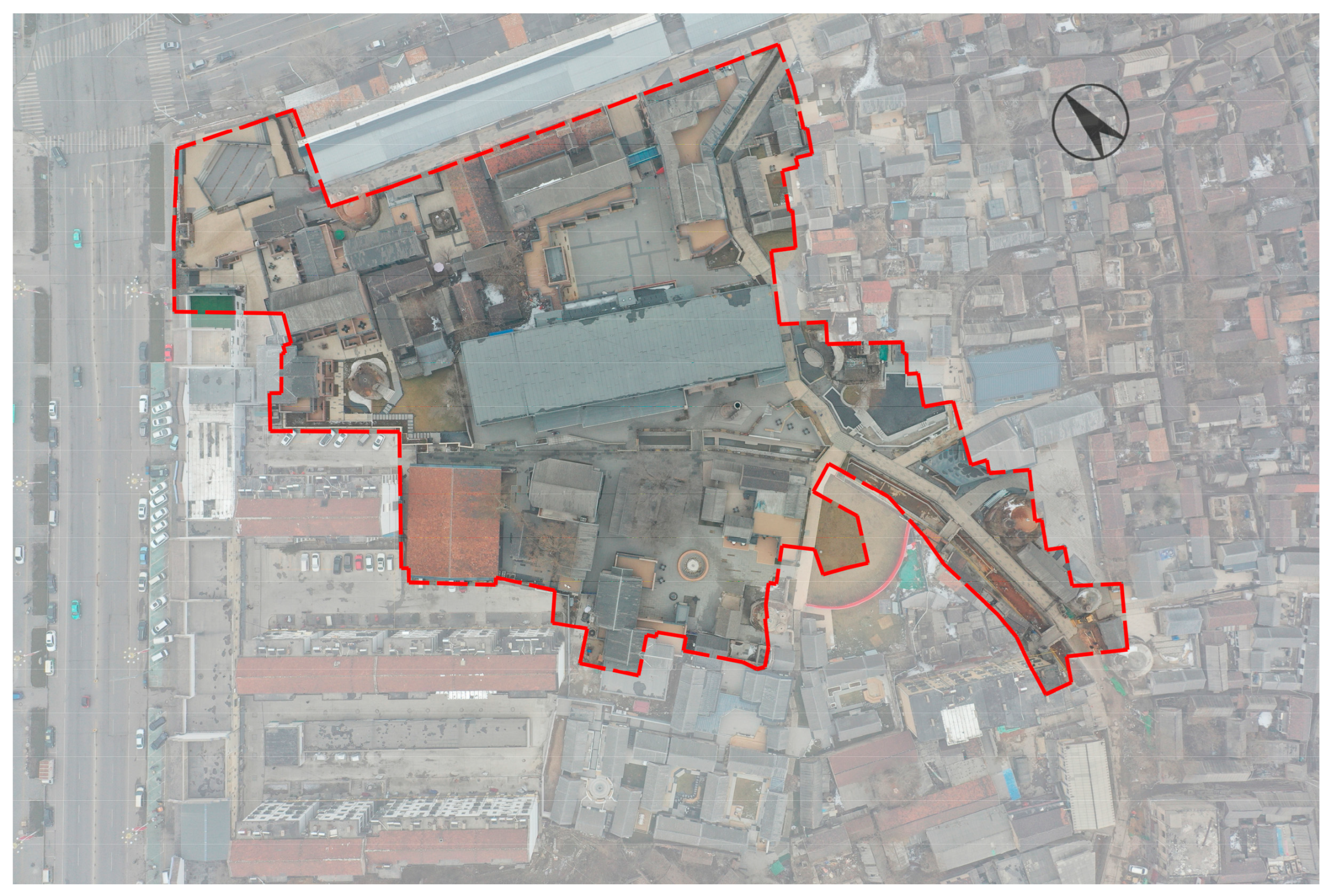
Figure 1. Real situation of the pottery production base in Taoliu Town, Zibo City.
Sustainability 14 11622 g001
Figure 2. Main pollution sources of atmospheric particulate matter in the pottery production base of Taoliu Town.
Sustainability 14 11622 g002
Figure 3. Weather station.
Sustainability 14 11622 g003
Figure 4. Monitoring points (“a” stands for the small weather station, which can measure wind speed, wind pressure, wind direction, temperature, humidity, PM2.5, PM10, and solar radiation; “b” stands for the hand-held detector, which can measure wind speed, wind pressure, and PM2.5).
Sustainability 14 11622 g004
Figure 5. Linear regression analysis results of measured and simulated wind speeds in the study area.
Sustainability 14 11622 g005
Figure 6. Windward and leeward sides of the prevailing wind direction in summer.
Sustainability 14 11622 g006
Figure 7. Windward and leeward sides of the prevailing wind direction in winter.
Sustainability 14 11622 g007
Figure 8. PM2.5 concentration distribution at the cross-section of Y = 3 m and an angle of 45° in summer and winter.
Sustainability 14 11622 g008
Figure 9. PM2.5 concentration distribution at the cross-section of Y = 3 m and an angle of 90° in summer and winter.
Sustainability 14 11622 g009
Figure 10. PM2.5 concentration distribution for enclosed vegetation (F1–F2) at the cross-section of Z = 1.5 m.
Sustainability 14 11622 g010
Figure 11. PM2.5 concentration distribution for incremental vegetation (F3–F4) at the cross-section of Z = 1.5 m.
Sustainability 14 11622 g011
Figure 12. PM2.5 concentration distribution for centralized vegetation (F5–F6) at the cross-section of Z = 1.5 m.
Sustainability 14 11622 g012
Figure 13. PM2.5 concentration distribution for the distance of 1 m between plants and buildings at the cross-section of Z = 1.5 m.
Sustainability 14 11622 g013
Figure 14. PM2.5 concentration distribution for the distance of 2 m between plants and buildings at the cross-section of Z = 1.5 m.
Sustainability 14 11622 g014
Figure 15. PM2.5 concentration distribution for the distance of 3 m between plants and buildings at the cross-section of Z = 1.5 m.
Sustainability 14 11622 g015
Figure 16. Simulated cloud atlas of PM2.5 concentrations at the cross-section of Y = 6 m with different heights of vegetation and buildings on both sides.
Sustainability 14 11622 g016
Figure 17. PM2.5 concentration distribution for a building height of H = 3 m on both sides at the cross-section of Z = 0.5 m, 1.5 m, 2.5 m.
Sustainability 14 11622 g017
Figure 18. PM2.5 concentration distribution for a building height of H = 6 m on both sides at the cross-section of Z = 0.5 m, 1.5 m, 2.5 m.
Sustainability 14 11622 g018
Figure 19. PM2.5 concentration distribution for a building height of H = 9 m on both sides at the cross-section of Z = 0.5 m, 1.5 m, 2.5 m.
Sustainability 14 11622 g019
Figure 20. PM2.5 concentration distribution for a building height of H = 12 m on both sides at the cross-section of Z = 0.5 m, 1.5 m, 2.5 m.
Sustainability 14 11622 g020
Figure 21. PM2.5 concentration distribution for the street tree configuration of H1–H2 at the cross-section of Z = 1.5 m.
Sustainability 14 11622 g021
Figure 22. PM2.5 concentration distribution for the street tree configuration of H4–H5 at the cross-section of Z = 1.5 m.
Sustainability 14 11622 g022
Figure 23. PM2.5 concentration distribution for the street tree configuration of H6–H7 at the cross-section of Z = 1.5 m.
Sustainability 14 11622 g023
Figure 24. PM2.5 concentration distribution for the street tree configuration of H3–H8 at the cross-section of Z = 1.5 m.
Sustainability 14 11622 g024
Table 1. Typical layout of vegetation in Taoliu Town, Zibo City.
Sustainability 14 11622 i001Sustainability 14 11622 i002Sustainability 14 11622 i003Sustainability 14 11622 i004
D1D2D3D4
Table 2. Types of vegetation community (1:100).
EnclosedIncrementalCentralized
Sustainability 14 11622 i005Sustainability 14 11622 i006Sustainability 14 11622 i007Sustainability 14 11622 i008Sustainability 14 11622 i009Sustainability 14 11622 i010
F1F2F3F4F5F6
Table 3. Types of street tree combinations (1:100).
Sustainability 14 11622 i011Sustainability 14 11622 i012Sustainability 14 11622 i013Sustainability 14 11622 i014
H1H2H3H4
Sustainability 14 11622 i015Sustainability 14 11622 i016Sustainability 14 11622 i017Sustainability 14 11622 i018
H5H6H7H8
Note: H1 and H8 are simplified from real scenes, and H2–H7 represent random combinations of various plants.
Table 4. Grid density setting.
Wind DirectionModeling AccuracyGrid TypeAmplification Coefficient of Boundary LayerNumber of Grids
NE2/4Non-structural tetrahedral grid1.21,317,682
SSW2/4Non-structural tetrahedral grid1.214,827,530
Table 5. Evaluation standards for air-pollutant-concentration levels.
NameAir Quality IndexAir Quality GradeAir Quality Level
P1AQI ≤ 50Grade 1Good
P250 < AQI ≤ 100Grade 2Moderate
P3100 < AQI ≤ 15Grade 3Light polluted
P4150 <AQI ≤ 200Grade 4Medium polluted
P5200 < AQI ≤ 300Grade 5Heavy polluted
P6AQI > 300Grade 6Severe polluted
Table 6. Validation of measured wind speed PM2.5 concentration and simulated values.
ItemCategoryMean ValueStandard Deviationtdfsig
Wind speedMeasurement0.890.232.2160.078
Simulation0.850.22
PM2.5Measurement97.114.122.2660.065
Simulation87.928.68
Table 7. Plant configuration table.
Scientific NameSpeciesFamily NameApplication RangeSize, ShapeMaterial ObjectModel
Quercus L.Deciduous broadleaf treesFagaceaeGap6 m high, with a canopy width of about 3 m, conicalSustainability 14 11622 i019Sustainability 14 11622 i020
Populus davidiana DodeDeciduous treesWillow familyTwo sides of buildings, forest margins, open forests5 m high, with a canopy width of about 2–2.6 m, ovalSustainability 14 11622 i021
Betula platyphylla SukaczevDeciduous treesBetulaceaeGaps, two sides of buildings5 m high, with a canopy width of about 2–2.6 m, ovalSustainability 14 11622 i022
Lespedeza bicolor Turcz.Erect shrubsRosaceae LeguminosaeForest margins, gaps, outside of viaducts2–3.5 m high, with a canopy width of about 1.5–2.5 m, long oval
Sustainability 14 11622 i023Sustainability 14 11622 i024
Ilex Chinensis SimsCasuarinaHolly familyNorthside of the building, open forest2–2.5 m high, with a canopy width of about 1.2–1.8 cm, spherical Sustainability 14 11622 i025
Acer palmatum Thunb.Small deciduous treesMaple familyForest margins1.5–2.5 m high, with a canopy width of about1.5–2 m, ovalSustainability 14 11622 i026
Amygdalus triloba (Lindl.) RickeShrubs and small treesRosaceaeBoth sides of the building, forest margins1–2.5 m high, with a canopy width of about 1–1.5 m, ovalSustainability 14 11622 i027
Arundinella anomala Steud.HerbsGramineaeForest margins, both sides of buildings0.6–1.1 m high, with a canopy width of about 0.5 m, ovalSustainability 14 11622 i028Sustainability 14 11622 i029
Themedajaponica (Willd.) TanakaHerbsGramineaeOpen forests, forest margins0.7–1.5 m high, with a canopy width of about 0.7–0.8 m, long circularSustainability 14 11622 i030
Publisher’s Note: MDPI stays neutral with regard to jurisdictional claims in published maps and institutional affiliations.