Abstract
The occurrence of premature rockbolt failure in underground mines has remained one of the most serious challenges facing the industry over the years. Considering the complex mechanism of rockbolts’ failure and the large number of influencing factors, the prediction of rockbolts’ failure from laboratory testing may often be unreliable. It is therefore essential to develop new models capable of predicting rockbolts’ failure with high accuracy. Beyond the predictive accuracy, there is also the need to understand the decisions made by these models in order to convey trust and ensure safety, reliability, and accountability. In this regard, this study proposes an explainable risk assessment of rockbolts’ failure in an underground coal mine using the categorical gradient boosting (Catboost) algorithm and SHapley Additive exPlanations (SHAP). A dataset (including geotechnical and environmental features) from a complex underground mining environment was used. The outcomes of this study indicated that the proposed Catboost algorithm gave an excellent prediction of the risk of rockbolts’ failure. Additionally, the SHAP interpretation revealed that the “length of roadway” was the main contributing factor to rockbolts’ failure. However, conditions influencing rockbolts’ failure varied at different locations in the mine. Overall, this study provides insights into the complex relationship between rockbolts’ failure and the influence of geotechnical and environmental variables. The transparency and explainability of the proposed approach have the potential to facilitate the adoption of explainable machine learning for rockbolt risk assessment in underground mines.
1. Introduction
Rockbolts are the most widely adopted support system for stabilising excavations in underground mines, due to their justified reliability in rock reinforcement [1,2,3]. They are primarily used to restrain rock mass deformation by suspending weaker rock layers onto more competent ones. In underground mining operations, bolts have been used to support surrounding rock masses [4,5,6,7], roadways [8,9,10], mining shafts [11,12], and as reinforcement of pillars [13]. However, rockbolts, like any ground support system, may only delay collapse for some time [14]. Therefore, the ability of rockbolts to sustain the weight of unstable blocks throughout the mine’s life is crucial to ensure effective exploitation in the context of economics and safety.
Over the past years, there has been an increasing number of rockbolt failures around the world, usually as a result of stress corrosion cracking (SCC) and localised pitting corrosion [15,16,17,18]. Craig et al. [3] identified sulphate-reducing bacteria as a causative agent of SCC and localised corrosion. In a study by Wu et al. [19], mineralogical materials were found to indirectly enhance the rate of corrosion by increasing the concentration of total dissolved solids. Other influencing factors of rockbolt failures identified in the literature include an increase in horizontal stress on bolts and the presence of groundwater and clay bands within the bolting horizon [1,15]. The varying conditions are indicative of the complex relationship existing between rockbolts’ failure and the influencing parameters in a typical underground mine. In effect, attempts to predict such failures via laboratory tests are mostly ineffective, because they fail to represent the complex mining environment [20].
In response to these challenging requirements, an indirect risk assessment of rockbolts’ failure using machine learning (ML) models is proposed in the literature [20]. The advantages of ML models lie in their ability to accommodate more input variables (categorical or numeric) and sufficiently model nonlinear and complex relationships between variables. Jiang et al. [20] utilised a support-vector machine (SVM) as an ML method to predict the risk (high or low) of rockbolts’ failure using geotechnical and environmental input variables. The predicted failures were consistent with the ground truth, with an AUC of 0.85 and 0.86 on the training and testing datasets, respectively. In similar studies, such as the work of Sun et al. [21], ML (probabilistic neural network) was successfully used to detect rockbolts’ defects. Zheng et al. [22] reported a bolt-defect-recognition rate of 95.45% using an SVM. In a recent study by Singh et al. [23], an artificial neural network was used to classify roof bolts with a quality identification of around 80%. Other studies have also employed ML for predicting the corrosion behaviour [24,25] and crack growth rate in Type 304 stainless steel [26]. Although remarkable predictive performances have been achieved in previous studies, there is still the need to explore the applicability of new ML models. This is because no single ML model can be universally/consistently efficient for assessing the risk of rockbolts’ failure, according to the “no free lunch” theorem [27]. Moreover, the introduction of new ML models to improve predictive performance is a valid goal for research.
Beyond predictive performance, there is a growing concern about these models’ “black box” nature, which makes it difficult for end-users to comprehend why and how particular decisions are reached [28]. After all, models should not only be good, but also interpretable [29]. More importantly, end-users should be aware of when the models fail. It is worth noting that ML models are mostly unable to accurately generalise beyond patterns seen during training, yet they still give predictions (usually wrong) with high confidence for out-of-distribution samples [30]. In critical safety domains such as the risk assessment of rockbolts’ failure (in underground mines), it is essential to know the reasons why ML models make certain predictions, because incorrect results may have significant consequences. Questions such as (i) why a sample was correctly classified as having a high and not a low risk of failure, and (ii) how (in terms of direction) influencing variables drive models’ prediction, need to be addressed. Previous studies, such as the work of Jiang et al. [20], have employed methods such as relative feature importance to understand the importance of predictor variables on rockbolts’ failure. However, such methods are unable to determine the relationships existing between the input and output variables. Additionally, relative feature importance is often biased toward high-cardinality features and cannot determine the contribution of input features to the generalisable predictive performance (i.e., performance on unseen data). Therefore, there is the need to develop new models that can accurately recognise high or low risk of bolt failure, while simultaneously providing the underlying reasoning behind their decisions.
In this regard, a very new ML model—namely, categorical gradient boosting (Catboost)—was used to predict the risk of rockbolts’ failure in an underground coal mine. The performance of the Catboost model was assessed and compared with a random forest (RF) model. Then, a comprehensively novel model explainability approach using SHapley Additive exPlanations (SHAP) was employed to explain the models’ decisions. SHAP interpretation can help fill the gaps in understanding of rockbolts’ failure in complex mining environments, and can also convey trust in the use of ML in the real-time risk assessment of failure. The remainder of this paper is organised as follows: The next two sections (Section 2 and Section 3) present the case study and methodology, respectively. In Section 4, the results obtained and the corresponding discussion are presented. The conclusions of this study are then presented in the final section.
2. Case Study
This study makes use of an existing database [20] consisting of cases of premature bolt failure in an underground coal mine in New South Wales, Australia. The dataset consists of 160 instances of roof panels with 12 features representing the geotechnical and environmental conditions of the site. A summary of the dataset is presented in Table 1, while the distribution of the continuous features is shown in Figure 1. The data contains four continuous variables (“dripper flow rate”, “age of bolts”, “length of roadway”, and “stress factor”) and eight categorical features (representing three zones and five locations). Roof panels with fallen bolts are labelled as having a high risk of failure, while a low risk of failure is assigned to those with no fallen bolts. A detailed description of the dataset is presented in the study of Jiang et al. [20].

Table 1.
Variables used for the modelling.
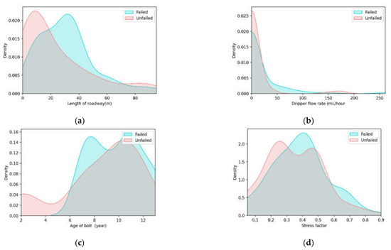
Figure 1.
Kernel density estimate plots of four continuous features: (a) length of roadway; (b) dripper flow rate; (c) age of bolt; (d) stress factor.
3. Methods
3.1. Model-Building Process
In this study, the 12 input features (presented in Table 1) were used as input variables to predict the risk of rockbolts’ failure (high-risk or low-risk). The model-building workflow is presented in Figure 2. According to Figure 2, the database was randomly split into a training set (80%) and a testing set (20%). Here, stratified sampling was employed to ensure that an equal proportion of the high and low risks occurred in the training and testing sets. The training set was used to train the ML models through a 5-fold cross-validation.
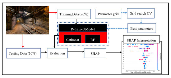
Figure 2.
Workflow of the entire study.
Gridsearch was used to obtain the best parameter pairs to ensure optimal performance. The tuning parameters for Catboost and RF were limited to 3 and 2, respectively, to ensure simpler models. The Gridsearch parameter relationship with cross-validation performance for Catboost and RF is shown in Figure 3a,b, respectively. Python-based ML libraries known as Catboost [31] and Scikit-learn [32] were employed to build the Catboost and RF models, respectively.
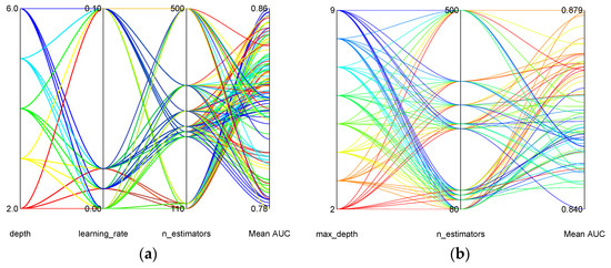
Figure 3.
Relationship of Gridsearch parameters with mean AUC: (a) Catboost; (b) RF.
For Catboost, the best parameter combination was obtained with depth = 6, learning_rate = 0.01 and n_estimators = 110. The learning_rate is used for reducing the gradient step, the depth represents the depth of the tree, and the n_estimators represent the maximum number of trees that can be built. With RF, the optimal model was obtained with the parameters; max_depth = 3 and n_estimators = 500. Similarly, the max_depth represents the maximum depth of the tree, and the n_estimators represent the number of trees in the forest.
The best parameters were finally used to retrain the models. Then, the testing dataset, containing only the predictor variables, was supplied to the models to make predictions. The predictions were then evaluated to assess and compare the models’ generalisation performances. Finally, SHAP was employed to explain the predictions of the Catboost model. The theoretical background of Catboost and SHAP is presented in the following subsections. The RF model is not discussed in this study because it has been detailed extensively in the literature [33,34,35,36].
3.2. Categorical Boosting (Catboost)
Catboost, proposed by Prokhorenkova et al. [31], is a powerful open-source gradient boosting algorithm efficient in handling both regression and classification tasks. Its implementation introduces two new advances to the boosting family: (i) ordered boosting to solve the problem of prediction shifts present in all existing implementations of gradient boosting, and (ii) an innovative technique to handle categorical variables [31].
The algorithm has demonstrated superiority over leading boosting variants for a variety of problems. For instance, in the study of Luo et al. [37], Catboost achieved good performance compared to RF and extreme gradient boosting. In the work of Prokhorenkova et al. [31], Catboost performed better than light gradient boosting and extreme gradient boosting. In a recent comparison by Wu et al. [38], Catboost demonstrated remarkable predictive capabilities compared to existing boosting algorithms. Particularly in the geotechnical discipline, the algorithm has been widely applied—especially in predicting uniaxial compressive strength [39], prediction of the elastic modulus of rocks [40], and rock burst assessment [41].
The underlying strategy of Catboost, like all other boosting techniques, is to learn many weak classifiers (i.e., base learners) and combine them into a stronger one. In the Catboost implementation, a binary decision tree is used as the base classifier. The decision tree divides the feature space () into several disjointed tree nodes using some splitting attribute (a). The attribute consists of a single feature (k) and a threshold (), where k is either a numeric or a binary feature. In the case of this study, the attributes consist of binary variables and numeric variables that are used to identify whether a feature exceeds some threshold. For numeric features (e.g., “age of bolt”), , while for binary features (“zone 2”), [31]. It is worth noting, however, that the decision tree is unable to process categorical variables in the input data. Hence, in the existing boosting methods, one-hot encoding is employed to add a new binary feature, which indicates the presence or absence of each feature [42]. However, in high-cardinality datasets (i.e., when there are too many unique categories for a feature), this approach leads to space consumption.
In handling the aforementioned limitation of the one-hot encoding, one common approach is to replace the unique category of the categorical feature i with some target statistics (TS), . Considering a dataset , where represents the input variables containing both numeric and categorical features, while represents the target class, the TS is defined in Equation (1) as follows:
where a > 0 is a parameter and p is generally the average target value in the dataset [43]. However, this approach also leads to overfitting. Catboost uses a more efficient strategy known as the ordered TS, which helps to reduce overfitting. Here, the dataset is first permutated randomly. Then, an average label value is computed for each example with the same category value placed before the inherited one from the permutation in the dataset. If represents the permutation, then is replaced in Equation (2) as follows:
where p is the prior value and a is the weight of the prior.
3.3. SHapley Additive exPlanations (SHAP)
In this study, the tree-explainer-based SHAP [44] framework with Catboost was employed to explain the complex underlying relationships among the influencing factors of rockbolts’ failure. SHAP, introduced by Lundberg and Lee [44], is a game-theory-based approach used to describe the outcomes of ML models by determining the contribution of each predictor variable to the models’ output. Here, contributions are estimated by computing Shapley values [45] for individual instances.
As a game theory approach, each predictor variable acts as a player in a coalition. Then, the payoff (contribution), which represents the increase in the probability of a particular class (high- or low-risk) occurring when conditioning the feature, is estimated. The outcome of the model is explained using the concept of additive feature attribution. SHAP specifies the explanation in Equation (3) as follows:
where g represents the explanation model, is a coalition vector that indicates whether the ith predictor is present () or absent (), is the base value when all inputs are unavailable, and M is the maximum coalition size. is the Shapley value, which represents feature attribution for a feature i. For a model f, the Shapley value () is calculated in Equation (4) as follows:
where S represents the subset of features used in the model, is the vector of feature values of the observation to be explained, and M represents the number of features; is the prediction for feature values in set S.
Since SHAP computes Shapley values, it is known to be the only method that satisfies all of the properties of efficiency, symmetry, dummy, and additivity [46]. Interestingly, SHAP is justified to provide a unique solution with three vital properties: local accuracy, consistency, and missingness [44,46,47]. The desirable properties of SHAP have led to its increasing adoption in the geotechnical discipline. A review of some successful applications of SHAP is presented in Table 2.
Table 2.
Review of some applications of SHAP in the geotechnical engineering domain.
4. Results and Discussion
4.1. Classification Performance
In section, the performance of Catboost and RF are assessed and compared. The performance of the models was evaluated using overall (AUC) and single-class (precision and sensitivity) performance metrics. The corresponding formulae (Equations (5)–(7)) for these metrics are provided in Table 3.
Table 3.
Evaluation metrics with formulae and descriptions.
The performance of the proposed Catboost model was further evaluated by comparing its performance with the results obtained for other ML methods by Jiang et al. [20]. The results are summarised in Table 4. In comparison with the results presented by Jiang et al. [20], the Catboost model used in this study produced satisfactory results (Table 4).
Table 4.
Classification performance of the various models developed for the study and the models used by Jiang et al. [20].
To aid in easy interpretation, confusion matrices of the classification results for Catboost and RF are additionally presented in Figure 4a,b, respectively. Overall, the results indicate that the newly introduced Catboost model provides better prediction than the RF model in terms of AUC, achieving the highest score of 0.89 and 0.88 on the training and testing datasets, respectively (Figure 5). This means that the Catboost model has the highest discrimination ability to distinguish between the high- and low-risk rockbolt failures.
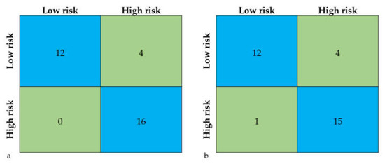
Figure 4.
Confusion matrices for (a) Catboost and (b) RF.
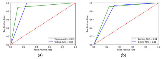
Figure 5.
AUC plots for training and testing datasets: (a) Catboost; (b) RF.
The single-class performance also revealed that the Catboost model was the most efficient in recognising both high- and low-risk zones (Figure 6). In risk assessment, high sensitivity of a model in detecting areas at high risk of failure is of utmost importance, since it serves as a safety buffer. The Catboost model developed in this study achieved a high sensitivity of 1 (Figure 6), indicating that all high-risk failures were correctly classified or identified by the model. As indicated in Figure 4a, Catboost correctly classified all of the high-risk cases, and only committed four of the low-risk cases. Further explanation of such model classification is discussed in subsequent sections.
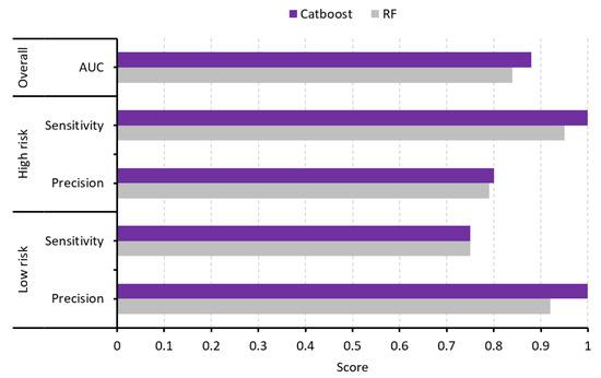
Figure 6.
Overall and single-class performance for Catboost and RF.
4.2. SHAP Global Interpretation
The SHAP feature importance plot (Figure 7a) gives the average contribution of a feature value to the prediction for the six most important variables or features. The features are sorted in decreasing importance. It was observed that “length of roadway” (f1) and “headgate 1” (f8) were the greatest contributing factors; f1 was similarly identified in a previous study [20] as the most important variable. However, the overall importance ranking obtained in this study (f1, f8, f3, f11, f9, f4) differs from that given by the gradient tree boosting (GTB) model (f1, f2, f4, f3, f10, f8, f11, f9, f5, f6, f12, and f7) used by Jiang et al. [20]. In the study of Jiang et al. [20], all numeric values (f1, f2, f3, and f4) were ranked higher than the binary features. This is because the GTB model employs its internals to compute the importance calculated using a weighted sum of decreases in node impurity, making it inherently biased toward numeric features (i.e., higher cardinality) [47].
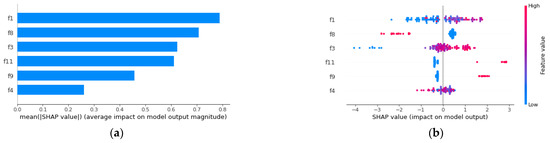
Figure 7.
Global SHAP interpretations of predictions on the training dataset: (a) feature importance plot; (b) summary plot showing the first six important variables (note: f1 is in m).
The directional marginal contribution of the six most important predictor variables to the various classes is presented in Figure 7b. Here, each point on the plot corresponds to a row in the dataset. The gradient colour of each point represents the magnitude of the input variable i.e., red or blue plots represent higher or lower values of inputs, respectively. The y-axis represents the variable names, ranked from top to bottom in order of importance (similarly depicted in Figure 7a); the x-axis depicts the SHAP value. The points are coloured on both sides for all features, indicating how much a feature impacts the model negatively (left) or positively (right).
It can be observed in Figure 7b that the medium-to-high values of f1 increase the risk of rockbolt failures, and vice versa. With regards to f8, category 1 (indicating rockbolts located in “headgate 1”) indicates the lowest risk of failure (Figure 7b). This means that rockbolts located in “headgate 1” have the lowest risk of failing. In terms of “age of bolt” (f3), old bolts have a higher risk of failure, while new bolts generally have a low risk of failure (Figure 7b). There is also a high risk of bolt failure in “cut-through 2” (f11) and “cut-through 1” (f9). A high “stress factor” (f4) increases the risk of failure, and vice versa (Figure 7b). On the other hand, “dripper flow rate” (f2) and rockbolts in “zone 1” (f5), “zone 2” (f6), “zone 3” (f7), and “headgate 2” (f10) generally have less impact on failure outcomes; however, in some instances, a high “dripper flow rate” is observed to increase the risk of failure (Figure 7b). It is important to note that in determining the risk of a rockbolt’s failure, the most important factors should be considered first followed by the preceding factors in importance.
The relationships between SHAP values and the input variables are shown in Figure 8. The colour coding on the right relates to the values for the interaction feature. Vertical dispersion of points represents interaction among predictor variables. The deductions from the dependency plots can be summarised as follows:
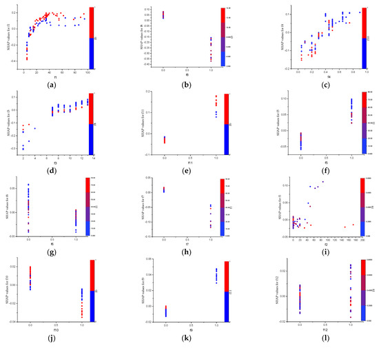
Figure 8.
SHAP dependency and interaction effect plots for various input parameters (note: f1, f2, and f3 have units of m, mL/h, and years, respectively).
- Figure 8a indicates that rockbolts with “length of roadway” greater than 30 m are more likely to fail (i.e., SHAP values > 0). The risk even increases when the roadway is located in “zone 2”.
- In Figure 8b, one can observe that rockbolts existing in “headgate 1” are less likely to fail, and vice versa.
- Again, rockbolts with a “stress factor” value less than 0.3 are less likely to fail (Figure 8c). The probability of failure decreases even further when the rockbolts are located at “headgate 2”. However, the risk of failure increases with increasing “stress factor”.
- Figure 8d shows that rockbolts with age of less than 5 years are very unlikely to fail. After 5 years, the risk of failure increases with time.
- In Figure 8e, it can be seen that rockbolts located in “cut-through 2” are more likely to fail. Additionally, bolts in “cut-through 2” within “zone 2” have a higher risk of failure.
- According to Figure 8f, rockbolts in “zone 1” with a “length of roadway” less than 20 m are more likely to fail.
- Rockbolts in “zone 2” and “zone 3” are less likely to fail, as shown in Figure 8g,h, respectively.
- The “dripper flow rate” generally has less impact on bolt failure; however, a “dripper flow rate” of 40–60 mL/h together with a low “stress factor” could potentially cause failure (Figure 8i).
- The risk of failure in “headgate 2” is very low and is even more unlikely to fail when “headgate 2” is located in “zone 2” (Figure 8j).
- Figure 8k shows that rockbolts located in “cut-through 1” have the potential to fail, although the probability is less.
- Figure 8l shows that “headgate 3” generally does not have a serious impact on failure.
We caution that the above-listed conditions are ranked in order of importance, and so any sample should be interpreted by subjecting it to the various conditions in order of importance. For instance, in condition VII, rockbolts in “zone 2” and “zone 3” are less likely to fail. However, in condition I, rockbolts with a longer “length of roadway” have the highest risk of failure when they are located in “zone 2”. Additionally, bolts in “cut-through 2” and “zone 2” have a higher risk of failure. Moreover, rockbolts in “zone 1” with a “length of roadway” less than 20 m are more likely to fail. The findings reported by Jiang et al. [20] suggested that zones 1, 2, and 3 (indicating three water types) were less important to the prediction outcome. Conversely, the SHAP dependency plot and the interaction features from this study suggest otherwise. It can be established from our findings that water types in conjunction with other variables are important contributing variables for rockbolts’ failure [1]. Our results also establish that the risk of rockbolts’ failure could be localised in clusters [1].
4.3. SHAP Local Interpretation
Figure 9a presents the decision plot of all of the testing datasets. This gives an overall summary of the contribution of each predictor variable to the prediction outcomes. For instance, it can be seen that in areas with a high risk of failure, f1 generally contributes positively (right direction), whereas f7, f9, and f12 appear to have a neutral effect on the outcomes (Figure 9a).
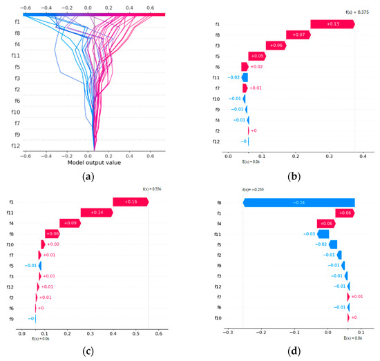
Figure 9.
Local interpretations of predictions on the testing dataset: (a) all testing samples; (b) sample 1; (c) sample 3; (d) sample 2 (note: f1, f2, and f3 have units of m, mL/h, and years, respectively).
The SHAP waterfall plots (Figure 9b–d) are instructive in explaining how individual decisions are taken. Here, the contribution of each predictor variable (positive/negative) to the predictions can be assessed. The f(x) value on top of the plot indicates the probability of a high risk of failure. Positive values represent higher risk, while negative values represent lower risk. The E[f(x)] values represent the expectation of a high risk of failure. The y-axis represents the variable name, and the corresponding observed values are presented in Table 5; the x-axis represents the range of responses.
Table 5.
Details of test samples used for local interpretation.
In Figure 9b, a rockbolt with low risk of failure is wrongly predicted as high risk of failure. To understand the cause of this incorrect prediction (i.e., low risk instead of high risk), global analysis derived from the dependency plots in Figure 8 was used. As shown in Figure 8, it has already been established that old rockbolts (f3 = 13 years) located outside “headgate 1” (f8 = 0) with higher f1 values (f1 = 75) have a high risk of failure. As evident from Figure 9b, these important variables drive the prediction positively toward a high risk of failure.
In Figure 9c, a rockbolt with a high risk of failure (i.e., f(x) = 0.556) is correctly predicted. Again, using the conditions outlined in Figure 8, it is clear that a rockbolt with high f1 values (f1 = 38) and located in “cut-through 2” (f11 = 1), in “zone 2” (f6 = 1), and with more than 0.3 “stress factor” (f4 = 0.4) will have a higher risk of failure.
In explaining the correct prediction of low failure risk in Figure 9d, it can be observed that the rockbolt’s location in “headgate 1” (f8 = 1) is the main contributor to the prediction. Even though the “stress factor” is more than 0.3, the location alone nullifies all possibilities of high failure risk by driving the prediction to the extreme left. This is consistent with the conditions established from the dependency plots in Figure 8.
5. Conclusions
In this study, a categorical boosting (Catboost) algorithm and SHapley Additive exPlanations (SHAP) were leveraged to conduct a risk assessment of rockbolts’ failure in underground coal mines in New South Wales, Australia. First, the Catboost model was developed to predict the risk of rockbolts’ failure (high or low) using 12 input features. The model obtained high AUC scores of 0.88 and 0.84 on the testing and training data, respectively. Specifically, it obtained a sensitivity of 1 and 0.75 in predicting high and low risks of failure, respectively. In comparison with RF, Catboost showed a better performance with regard to all assessment metrics. Finally, SHAP was used to explain the nonlinear complex relationship between rockbolts’ failure and influencing input features. The outcomes of the analysis revealed the following conclusions:
- “Length of roadway” was found to be the greatest contributing factor to the failure outcome, followed (in decreasing order of importance) by “headgate 1”, “stress factor”, “age of bolts”, “cut-through 2”, “zone 1”, “zone 2”, “zone 3”, “dripper flow rate”, “headgate 2”, “cut-through 1”, and “headgate 3”.
- Rockbolts with a “length of roadway” greater than 30 m are more likely to fail. This risk increases even further when groundwater with high sulphur content is present.
- Rockbolts with a service age less than 5 years are very unlikely to fail. After 5 years, the risk of failure increases with time.
Overall, this study provides insights into the complex relationship between rockbolts’ failure and the influence of geotechnical and environmental variables. The transparency and explainability of the proposed approach have the potential to facilitate the adoption of explainable machine learning for rockbolt risk assessment in underground mines. It is recommended that future studies consider adding the rock types and rock strength to the predictor variables, as well as assessing how the reconstruction of the input variables via autoencoders could improve performance.
Author Contributions
Conceptualisation, B.I. and I.A.; methodology, B.I.; software, B.I.; validation, B.I. and I.A.; formal analysis, B.I.; investigation, B.I.; resources, B.I.; data curation, B.I.; writing—original draft preparation, B.I.; writing—review and editing, B.I., I.A., and A.E.; visualisation, B.I.; supervision, I.A. and A.E. All authors have read and agreed to the published version of the manuscript.
Funding
This research received no external funding.
Institutional Review Board Statement
Not applicable.
Informed Consent Statement
Not applicable.
Data Availability Statement
Publicly available datasets were analysed in this study; these data can be found here: [https://doi.org/10.1002/asmb.2273].
Acknowledgments
The authors are grateful to Ismet Canbulat, Chengguo Zhang, and Chunchen Wei (all of the University of New South Wales) for their remarkable suggestions and guidance.
Conflicts of Interest
The authors declare no conflict of interest.
References
- Hebblewhite, B.; Lu, T. Geomechanical behaviour of laminated, weak coal mine roof strata and the implications for a ground reinforcement strategy. Int. J. Rock Mech. Min. Sci. 2004, 41, 147–157. [Google Scholar] [CrossRef]
- Emery, J.; Canbulat, I.; Zhang, C. Fundamentals of modern ground control management in australian underground coal mines. Int. J. Min. Sci. Technol. 2020, 30, 573–582. [Google Scholar] [CrossRef]
- Craig, P.; Ramandi, H.L.; Chen, H.; Vandermaat, D.; Crosky, A.; Hagan, P.; Hebblewhite, B.; Saydam, S. Stress corrosion cracking of rockbolts: An in-situ testing approach. Constr. Build. Mater. 2021, 269, 121275. [Google Scholar] [CrossRef]
- Sakhno, I.; Sakhno, S.; Isaienkov, O.; Kurdiumow, D. Laboratory studies of a high-strength roof bolting by means of self-extending mixtures. Min. Miner. Depos. 2019, 13, 17–26. [Google Scholar] [CrossRef]
- Peter, K.; Moshood, O.; Akinseye, P.O.; Martha, A.; Khadija, S.O.; Abdulsalam, J.; Ismail, L.A.; Emman, A.A. An overview of the use of rockbolts as support tools in mining operations. Geotech. Geol. Eng. 2021, 40, 1637–1661. [Google Scholar] [CrossRef]
- Małkowski, P.; Niedbalski, Z.; Majcherczyk, T.; Bednarek, Ł. Underground monitoring as the best way of roadways support design validation in a long time period. Min. Miner. Depos. 2020, 14, 1–14. [Google Scholar] [CrossRef]
- Krykovskyi, O.; Krykovska, V.; Skipochka, S. Interaction of rock-bolt supports while weak rock reinforcing by means of injection rock bolts. Min. Miner. Depos. 2021, 15, 8–14. [Google Scholar] [CrossRef]
- Jing, H.; Wu, J.; Yin, Q.; Wang, K. Deformation and failure characteristics of anchorage structure of surrounding rock in deep roadway. Int. J. Min. Sci. Technol. 2020, 30, 593–604. [Google Scholar] [CrossRef]
- Tang, B.; Cheng, H. Application of distributed optical fiber sensing technology in surrounding rock deformation control of tbm-excavated coal mine roadway. J. Sens. 2018, 2018, 8010746. [Google Scholar] [CrossRef]
- Singh, R.N.; Heidarieh Zadeh, A.M. Rock Bolt Reinforcement System to Stabilise Shaft Intersections and Pit Bottom Roadways during Underground Reconstruction. In Proceedings of the The 23rd US Symposium on Rock Mechanics (USRMS), OnePetro, Berkeley, CA, USA, 25 August 1982. [Google Scholar]
- Tsusaka, K.; Yamasaki, M.; Hatsuyama, Y. Rock deformation and support load in shaft sinking in horonobe url project. In Proceedings of the ISRM Regional Symposium-EUROCK 2009, OnePetro, Cavtat, Croatia, 29 October 2009. [Google Scholar]
- Beus, M. An approach to field testing and design of deep mine shaft in the western USA. In Shaft Engineering; Institute of Mining and Metallurgy: London, UK, 2005; pp. 58–68. [Google Scholar]
- Waclawik, P.; Snuparek, R.; Kukutsch, R. Rock bolting at the room and pillar method at great depths. Procedia Eng. 2017, 191, 575–582. [Google Scholar] [CrossRef]
- Merwe, V.d.; Nielen, J.; Madden, B.J.; Buddery, P. Rock engineering for underground coal mining: A practical guide for supervisors at all levels, mine planners and students. S. Afr. Inst. Min. Metall. 2010, 7, 30–31. [Google Scholar]
- Craig, P.; Serkan, S.; Hagan, P.; Hebblewhite, B.; Vandermaat, D.; Crosky, A.; Elias, E. Investigations into the corrosive environments contributing to premature failure of australian coal mine rock bolts. Int. J. Min. Sci. Technol. 2016, 26, 59–64. [Google Scholar] [CrossRef]
- Hebblewhite, B.; Fabjanczyk, M.; Gray, P. Premature Rock Bolt Failure, Acarp Project no C8008. In Australian Coal Association Research Program; Australian Coal Association: Australia, 2002. [Google Scholar]
- Crosky, A.; Smith, B.; Hebblewhite, B. Failure of rockbolts in underground mines in australia. Pract. Fail. Anal. 2003, 3, 70–78. [Google Scholar] [CrossRef]
- Crosky, A.; Smith, B.; Elias, E.; Chen, H.; Craig, P.; Hagan, P.; Vandermaat, D.; Saydam, S.; Hebblewhite, B. Stress corrosion cracking failure of rockbolts in underground mines in australia. In Proceedings of the 7th International Symposium on Rockbolting and Rock Mechanics in Mining, Aachen, Germany, 30–31 May 2012. [Google Scholar]
- Wu, S.; Ramandi, H.L.; Chen, H.; Crosky, A.; Hagan, P.; Saydam, S. Mineralogically influenced stress corrosion cracking of rockbolts and cable bolts in underground mines. Int. J. Rock Mech. Min. Sci. 2019, 119, 109–116. [Google Scholar] [CrossRef]
- Jiang, P.; Craig, P.; Crosky, A.; Maghrebi, M.; Canbulat, I.; Saydam, S. Risk assessment of failure of rock bolts in underground coal mines using support vector machines. Appl. Stoch. Models Bus. Ind. 2018, 34, 293–304. [Google Scholar] [CrossRef]
- Sun, X.-y.; Kang, F.-n.; Wang, M.-m.; Bian, J.-p.; Cheng, J.-l.; Zou, D. Improved probabilistic neural network pnn and its application to defect recognition in rock bolts. Int. J. Mach. Learn. Cybern. 2016, 7, 909–919. [Google Scholar] [CrossRef]
- Zheng, H.-Q.; Yang, Y.-R.; Sun, X.-Y.; Wen, C. Nondestructive Detection of Anchorage Quality of Rock Bolt Based on DS-DBN-SVM. In Proceedings of the 2018 International Conference on Machine Learning and Cybernetics (ICMLC), Chengdu, China, 15–18 July 2018; pp. 288–293. [Google Scholar]
- Singh, S.K.; Raval, S.; Banerjee, B. Roof bolt identification in underground coal mines from 3d point cloud data using local point descriptors and artificial neural network. Int. J. Remote Sens. 2021, 42, 367–377. [Google Scholar] [CrossRef]
- Kamrunnahar, M.; Urquidi-Macdonald, M. Prediction of corrosion behaviour of alloy 22 using neural network as a data mining tool. Corros. Sci. 2011, 53, 961–967. [Google Scholar] [CrossRef]
- Jiménez–Come, M.; Turias, I.; Trujillo, F. An automatic pitting corrosion detection approach for 316l stainless steel. Mater. Des. 2014, 56, 642–648. [Google Scholar] [CrossRef]
- Shi, J.; Wang, J.; Macdonald, D.D. Prediction of crack growth rate in type 304 stainless steel using artificial neural networks and the coupled environment fracture model. Corros. Sci. 2014, 89, 69–80. [Google Scholar] [CrossRef]
- Wolpert, D.H.; Macready, W.G. No free lunch theorems for optimization. IEEE Trans. Evol. Comput. 1997, 1, 67–82. [Google Scholar] [CrossRef]
- Deeks, A. The judicial demand for explainable artificial intelligence. Columbia Law Rev. 2019, 119, 1829–1850. [Google Scholar]
- Lipton, Z.C. The mythos of model interpretability: In machine learning, the concept of interpretability is both important and slippery. Queue 2018, 16, 31–57. [Google Scholar] [CrossRef]
- Escalante, H.J.; Escalera, S.; Guyon, I.; Baró, X.; Güçlütürk, Y.; Güçlü, U.; van Gerven, M.; van Lier, R. Explainable and Interpretable Models in Computer Vision and Machine Learning; Springer International Publishing: Cham, Switzerland, 2018. [Google Scholar]
- Prokhorenkova, L.; Gusev, G.; Vorobev, A.; Dorogush, A.V.; Gulin, A. Catboost: Unbiased boosting with categorical features. Adv. Neural Inf. Processing Syst. 2018, 31, 6639–6649. [Google Scholar]
- Pedregosa, F.; Varoquaux, G.; Gramfort, A.; Michel, V.; Thirion, B.; Grisel, O.; Blondel, M.; Prettenhofer, P.; Weiss, R.; Dubourg, V. Scikit-learn: Machine learning in python. J. Mach. Learn. Res. 2011, 12, 2825–2830. [Google Scholar]
- Breiman, L. Random forests. Mach. Learn. 2001, 45, 5–32. [Google Scholar] [CrossRef]
- Ibrahim, B.; Ewusi, A.; Ahenkorah, I.; Ziggah, Y.Y. Modelling of arsenic concentration in multiple water sources: A comparison of different machine learning methods. Groundw. Sustain. Dev. 2022, 17, 100745. [Google Scholar] [CrossRef]
- Ibrahim, B.; Majeed, F.; Ewusi, A.; Ahenkorah, I. Residual geochemical gold grade prediction using extreme gradient boosting. Environ. Chall. 2022, 6, 100421. [Google Scholar] [CrossRef]
- Peters, J.; De Baets, B.; Verhoest, N.E.; Samson, R.; Degroeve, S.; De Becker, P.; Huybrechts, W. Random forests as a tool for ecohydrological distribution modelling. Ecol. Model. 2007, 207, 304–318. [Google Scholar] [CrossRef]
- Luo, M.; Wang, Y.; Xie, Y.; Zhou, L.; Qiao, J.; Qiu, S.; Sun, Y. Combination of feature selection and catboost for prediction: The first application to the estimation of aboveground biomass. Forests 2021, 12, 216. [Google Scholar] [CrossRef]
- Wu, T.; Zhang, W.; Jiao, X.; Guo, W.; Hamoud, Y.A. Comparison of five boosting-based models for estimating daily reference evapotranspiration with limited meteorological variables. PLoS ONE 2020, 15, e0235324. [Google Scholar] [CrossRef]
- Shahani, N.M.; Kamran, M.; Zheng, X.; Liu, C.; Guo, X. Application of gradient boosting machine learning algorithms to predict uniaxial compressive strength of soft sedimentary rocks at thar coalfield. Adv. Civ. Eng. 2021, 2021, 2565488. [Google Scholar] [CrossRef]
- Shahani, N.M.; Zheng, X.; Guo, X.; Wei, X. Machine learning-based intelligent prediction of elastic modulus of rocks at thar coalfield. Sustainability 2022, 14, 3689. [Google Scholar] [CrossRef]
- Li, D.; Liu, Z.; Armaghani, D.J.; Xiao, P.; Zhou, J. Novel ensemble intelligence methodologies for rockburst assessment in complex and variable environments. Sci. Rep. 2022, 12, 1844. [Google Scholar] [CrossRef]
- Chapelle, O.; Manavoglu, E.; Rosales, R. Simple and scalable response prediction for display advertising. ACM Trans. Intell. Syst. Technol. 2014, 5, 1–34. [Google Scholar] [CrossRef]
- Micci-Barreca, D. A preprocessing scheme for high-cardinality categorical attributes in classification and prediction problems. ACM SIGKDD Explor. Newsl. 2001, 3, 27–32. [Google Scholar] [CrossRef]
- Lundberg, S.M.; Lee, S.-I. A unified approach to interpreting model predictions. Adv. Neural Inf. Processing Syst. 2017, 30. [Google Scholar]
- Shapley, L.S. Stochastic games. Proc. Natl. Acad. Sci. 1953, 39, 1095–1100. [Google Scholar] [CrossRef]
- Molnar, C.J.S. 5.10 Shap (Shapley Additive Explanations)|Interpretable Machine Learning. Available online: https://christophm.github.io/interpretable-ml-book/shap.html (accessed on 2 August 2022).
- Masís, S. Interpretable Machine Learning with Python: Learn to Build Interpretable High-Performance Models with Hands-on Real-World Examples; Packt Publishing Ltd.: Birmingham, UK, 2021. [Google Scholar]
- Inan, M.S.K.; Rahman, I. Integration of explainable artificial intelligence to identify significant landslide causal factors for extreme gradient boosting based landslide susceptibility mapping with improved feature selection. arXiv 2022, arXiv:2201.03225. [Google Scholar]
- Amin, M.N.; Khan, K.; Javed, M.F.; Ewais, D.Y.Z.; Qadir, M.G.; Faraz, M.I.; Alam, M.W.; Alabdullah, A.A.; Imran, M. Forecasting compressive strength of rha based concrete using multi-expression programming. Materials 2022, 15, 3808. [Google Scholar] [CrossRef] [PubMed]
- Zhang, L.; Lin, P. Multi-objective optimization for limiting tunnel-induced damages considering uncertainties. Reliab. Eng. Syst. Saf. 2021, 216, 107945. [Google Scholar] [CrossRef]
- Lee, H.-L.; Kim, J.-S.; Hong, C.-H.; Cho, D.-K.J.A.S. Ensemble learning approach for the prediction of quantitative rock damage using various acoustic emission parameters. Appl. Sci. 2021, 11, 4008. [Google Scholar] [CrossRef]
- Nasiri, H.; Homafar, A.; Chelgani, S.C. Prediction of uniaxial compressive strength and modulus of elasticity for travertine samples using an explainable artificial intelligence. Results Geophys. Sci. 2021, 8, 100034. [Google Scholar] [CrossRef]
- Kannangara, K.P.M.; Zhou, W.; Ding, Z.; Hong, Z. Investigation of feature contribution to shield tunneling-induced settlement using shapley additive explanations method. J. Rock Mech. Geotech. Eng. 2022, 14, 1052–1063. [Google Scholar] [CrossRef]
- Mangalathu, S.; Shin, H.; Choi, E.; Jeon, J.-S. Explainable machine learning models for punching shear strength estimation of flat slabs without transverse reinforcement. J. Build. Eng. 2021, 39, 102300. [Google Scholar] [CrossRef]
- Khan, A.U.; Salman, S.; Muhammad, K.; Habib, M. Modelling coal dust explosibility of khyber pakhtunkhwa coal using random forest algorithm. Energies 2022, 15, 3169. [Google Scholar] [CrossRef]
- Mangalathu, S.; Hwang, S.-H.; Jeon, J.-S. Failure mode and effects analysis of rc members based on machine-learning-based shapley additive explanations (shap) approach. Eng. Struct. 2020, 219, 110927. [Google Scholar] [CrossRef]
- Barkhordari, M.; Armaghani, D.; Fakharian, P. Ensemble machine learning models for prediction of flyrock due to quarry blasting. Int. J. Environ. Sci. Technol. 2022, 19, 8661–8676. [Google Scholar] [CrossRef]
- Wang, L.; Wu, J.; Zhang, W.; Wang, L.; Cui, W. Efficient seismic stability analysis of embankment slopes subjected to water level changes using gradient boosting algorithms. Front. Earth Sci. 2021, 9, 1179. [Google Scholar] [CrossRef]
- Guo, D.; Chen, H.; Tang, L.; Chen, Z.; Samui, P. Assessment of rockburst risk using multivariate adaptive regression splines and deep forest model. Acta Geotech. 2022, 17, 1183–1205. [Google Scholar] [CrossRef]
Publisher’s Note: MDPI stays neutral with regard to jurisdictional claims in published maps and institutional affiliations. |
© 2022 by the authors. Licensee MDPI, Basel, Switzerland. This article is an open access article distributed under the terms and conditions of the Creative Commons Attribution (CC BY) license (https://creativecommons.org/licenses/by/4.0/).