A Data-Driven Based Method for Pipeline Additional Stress Prediction Subject to Landslide Geohazards

Abstract

Pipelines that cross complex geological terrains are inevitably threatened by natural hazards, among which landslide attracts extensive attention when pipelines cross mountainous areas. The landslides are typically associated with ground movements that would induce additional stress on the pipeline. Such stress state of pipelines under landslide interference seriously damage structural integrity of the pipeline. Up to the date, limited research has been done on the combined landslide hazard and pipeline stress state analysis. In this paper, a multi-parameter integrated monitoring system was developed for the pipeline stress-strain state and landslide deformation monitoring. Also, data-driven models for the pipeline additional stress prediction was established. The developed predictive models include individual and ensemble-based machine learning approaches. The implementation procedure of the predictive models integrates the field data measured by the monitoring system, with k-fold cross validation used for the generalization performance evaluation. The obtained results indicate that the XGBoost model has the highest performance in the prediction of the additional stress. Besides, the significance of the input variables is determined through sensitivity analyses by using feature importance criteria. Thus, the integrated monitoring system together with the XGBoost prediction method is beneficial to modeling the additional stress in oil and gas pipelines, which will further contribute to pipeline geohazards monitoring management.

1. Introduction

The pipeline is an important means for oil and gas transportation. The safe operation of the pipeline is threatened by various factors including corrosion, third-party damage, natural disaster, etc. For pipelines in areas with complex geological conditions such as mountainous regions, landslides have always been considered a dominant challenge for continuous pipeline service [1,2,3]. In this respect, landslides always impose additional stress on the pipeline, which may further lead to local deformation and displacement [4,5]. Once the additional stress generated exceeds the material strength or there are defects such as cracks and metal loss in the deformation area, it will seriously damage structural integrity of the pipeline [6], resulting in catastrophic accidents such as rupture and leakage. For example, in 2008–2009, two consecutive pipeline landslide accidents appeared in Zhejiang, China [7]. The earlier one was dealt with in time, whereas the latter one caused an explosion. On 5 March 2019, a pipeline rupture and subsequent explosion occurred in Alborz in Iran, leading to the suspension of gas supply to more than 12,000 customers [8]. With the random characteristic of natural disasters, it is difficult to predict and analyze their impact on pipelines. An accurate monitoring method is of great significance for protective measures to be taken at an early stage [9]. Therefore, it is fundamental to develop advanced methods for pipeline state monitoring under complicated geological circumstances.

It is known from the field that changed position of the pipeline under landslides imposes additional stresses on the pipeline, which put the pipeline in an unstable stress state [10,11]. To assess the resulting additional stress, the stress-strain monitoring for the pipelines across complex geological terrains is employed as an effective way for pipe condition monitoring. The widely used stress monitoring methods are categorized as long distance-based and point-based measurement. For long-distance real-time pipeline monitoring, distributed optical fiber sensors installed parallel to the pipe body are commonly utilized, which combines data acquisition capability including strss-strain behavior of soil, temperature, and vibration measurement [12,13]. It should be noted that this technology suffers equipment stability problems over the course of a long lifespan. In addition, point-based measurement adopts strain gauge sensors to stick around the pipe wall for strain monitoring, and the additional stress was calculated based on the measured strain value [14]. It directly reflects the pipeline behavior when compared with long-distance pipeline monitoring. However, the accuracy of the strain measurement sensor is susceptible to the disturbance of the external environment, resulting in the introduction of unreliable data.

Pipeline strain and stress are typically regarded as indicators that reflect the impact of landsliding on the pipeline [15], but an individual strain monitoring system cannot clearly explain the pipeline and its surrounding environmental conditions simultaneously. To improve the reliability of stress evaluation, landslide-related monitoring is complementary to comprehensive pipeline stress analysis. The landslide-induced failure of oil and gas pipelines is a complex process involving many parameters. Separately from strain monitoring, surface deformation monitoring and geohazard inducing monitoring are considered for landslide management [16,17]. For example, disaster reduction stick equipment has been designed to simultaneously monitor the landslide on precipitation, soil water content, pore water pressure, slope displacement, and slope inclination [18]. In most application cases, the monitoring of pipeline landslides is limited to the monitoring of the landslide hazard without the involvement of pipe interaction. There is still a lack of research on the stress state of pipelines under landslide interference. As a result, the relationship between landslide deformation data and pipeline safety conditions has not been effectively established.

Although pipeline landslide research in terms of soil-pipe interaction analysis [19], landslide behavior [20], and pipeline failure probability prediction [21] have been widely investigated. There are still some research gaps in this field. On the one hand, limited research has been done on the combined landslide hazard and pipeline stress state analysis. On the other hand, the interference of invalid measurement data of pipeline stress-strain monitoring has not been fully considered. To fill this gap, this paper focuses on establishing the quantitative relationship between landslide movement and pipeline mechanical state based on multi-parameter monitoring data. Advanced data-driven technologies are adopted for the prediction of additional stress. With joint monitoring tools and predictive models, effective prevention measures can be taken to reduce the probability of pipeline failure caused by landslides, which further mitigates the hazard of landslides posed on the pipeline. It should be noted that the model is applicable to slope soil layers, that is, slope sediment or residual soil or sedimentary soil. The contributions of this paper can be concluded as:

• A multi-parameter integrated monitoring system was developed to monitor the pipeline and landslide conditions in a complex geologic environment.
• The data-driven based predictive model was proposed for additional stress evaluation under landslide movement.
• Field sites were selected for demonstration of the geohazard monitoring system, and the additional stress model was verified based on the on-site data.

The rest of this paper is arranged as follows: Section 2 presents the pipeline geohazards monitoring implementation process; Section 3 describes the proposed methodology for accurate prediction of the additional stress. Section 4 performs a case study to illustrate the feasibility and effectiveness of the methodology. Section 5 presents the conclusions of this paper.

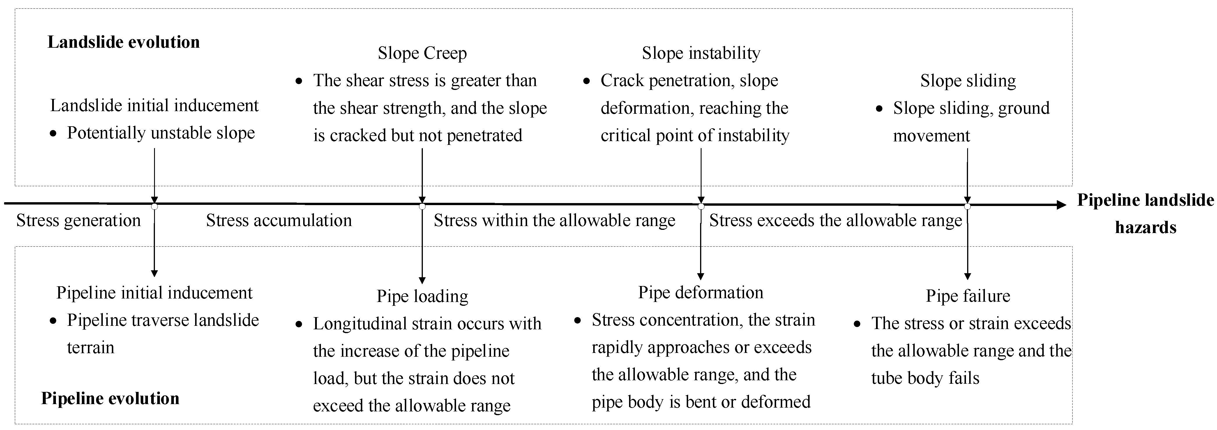
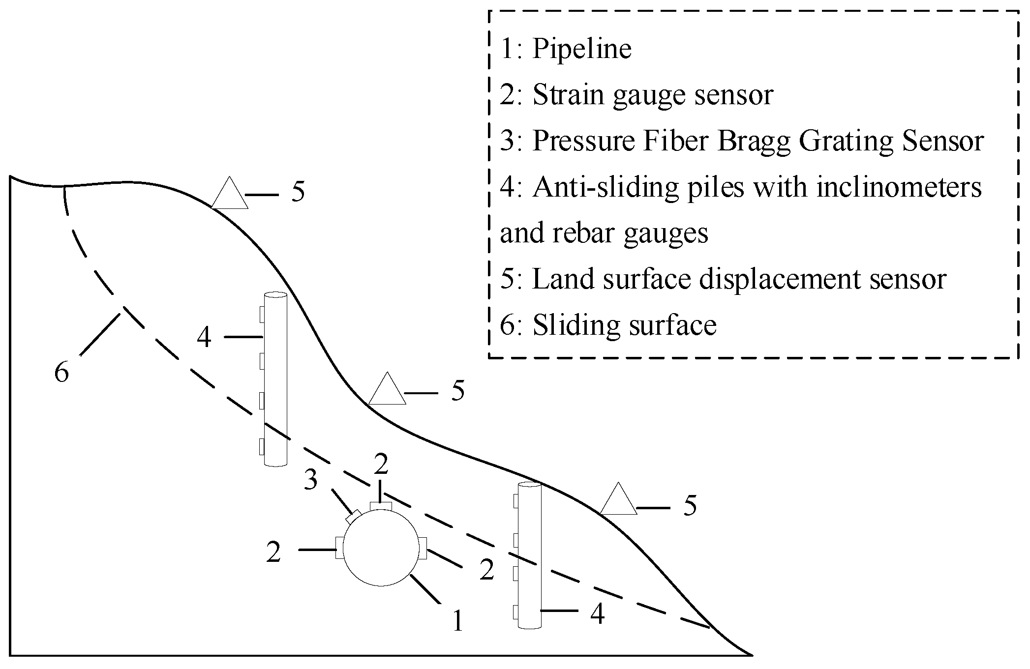
2. Pipeline Geohazards Monitoring Implementation

2.1. Selection of Monitoring Sites

In mountainous regions, it is impossible to avoid every potential landslide crossing. Pipelines passing through potentially active landslides may be subjected to forces such as traction, compression, and shear [22]. Due to the instability of the disaster-causing body, the stress concentration of the pipeline and the deformation of the pipe body lead to the occurrence of pipeline geological disasters. When the strain of the pipe body exceeds the allowable range, the pipe will bend and deform or even fail. The stability and deformation of landslides are affected by internal factors (soil composition, slope structure, geological structure, etc.) and external factors (water factors, weathering, earthquakes, human activities, etc.). Internal factors determine the scale and form of landslide deformation and failure, and external factors promote the occurrence and development of landslide deformation.

The landsliding process is a very complex process in which multiple factors are involved. For the pipeline landslide program, in addition to considering the scale of the landslide, it is also necessary to consider the impact of the landslide body on the pipeline structure. The evolution process of the pipeline landslide geological disaster was shown in Figure 1. The pipeline traversing landslide terrain is the initial inducement. In the early stage of landslide deformation, a certain part of the landslide body is deformed because the shear stress is greater than the shear strength, resulting in small creeping. During this period, the deformation rate of the landslide is characterized by low speed and stability, and the pipeline is slightly deformed. After that, with the gradual rupture of the slip surface, penetrated cracks begin to appear on the slope surface. With the increase of cracks, the slope body is in an unstable state, and the deformation of the pipeline increases. Finally, the slope sliding occurs and causes the failure of the pipeline.

Mitigation measures are usually implemented to eliminate or reduce the severity of landslide effects on the pipeline. It is economically feasible to install modern sensors in specific locations susceptible to ground movement. Pipeline monitoring points and landslide monitoring points are two important components of the integrated system. For the pipeline monitoring site, the selected monitoring points should reflect the force law of the critical pipeline segment, and the load distribution of the pipeline should also be considered. For the landslide deformation monitoring site, the monitoring data should comprehensively reflect the development of the landslide and its impact on the pipeline.

Some preliminary analysis is required for the selection of monitoring points before sensor installation. The steps are as follows. Firstly, the geohazard-sensitive areas of the pipeline are determined according to the engineering geological disaster report, geological survey report, and other relevant assessment documents. During this procedure, necessary investigations of slope maps, structural geology, morphology, surface mechanisms, and environmental conditions help to explain the mechanisms of landslide deformation and failure in specific situations. Secondly, site investigations in the selected geohazard-sensitive area will be conducted. The experts are also invited to further verify the key areas for controlling slope stability, and analyze the feasibility of equipment installation. Then, finite element simulations of the pipeline are carried out to determine the stress concentration point of the pipeline, and it was selected as the pipeline monitoring point.

2.2. Selection of Monitoring Elements

Generally, the content of pipeline landslide monitoring includes pipeline monitoring and landslide deformation monitoring. The monitoring of pipeline stress and strain can directly reflect the pipeline condition subject to geological hazards. In landslide monitoring, the monitoring contents are different with various requirements, among which surface displacement monitoring and inner displacement monitoring are the most important objects. For the inducing factors of geological disasters, the monitoring elements mainly include meteorological conditions such as rainfall, snowmelt, temperature, and evaporation, as well as hydrological conditions such as surface water, river, ditch water level, pore water pressure, soil moisture content, and groundwater level [23]. In this paper, parameters including pipeline additional stress, landslide surface displacement, landslide inner displacement, anti-sliding pile inclination, landslide traction stress and compressive stress, and soil pressure are selected as the monitoring indicators to form a joint monitoring system for pipeline landslide events.

2.2.1. Pipeline Monitoring

Additional stress. For landslides that have undergone large deformation, the pipelines laid in the slope body have been subjected to additional stress [24]. The strain gauge sensor attached to the surface of the pipeline is used to determine the additional stress for pipeline safety state evaluation. The strain gauges can easily capture the response of the pipeline to ground movement. This type of sensor uses elastic sensitive elements to measure the strain generated by the deformation of the object under force, and converts the external stress on the pipeline into the change of strength circuit. Therefore, by calculating the change of the current or voltage in the circuit, the external stress of the pipeline can be determined. Pipeline stress and strain monitoring are the core technologies of pipeline integrity management. It can intuitively and quantitatively obtain the real-time stress and strain data of the pipe body under buried working conditions and issue deformation warnings in time. Compared with land displacement monitoring, it reflects pipe deformation quickly and accurately. In order to obtain the accurate axial strain of the pipeline, at least 3 strain gauges should be arranged in each pipeline section.

2.2.2. Landslide Deformation Monitoring

Surface land displacement. The sliding of the soil mass on the surface of the landslide will have a direct impact on the pipelines buried in it. As the pipelines are mostly buried in trenches, floods and debris flows can easily wash away the upper soil of the pipelines, resulting in exposed pipelines. Moreover, soil accumulated around the pipelines will lead to excessive external stress, resulting in pipeline bending with serious consequences. Therefore, it is necessary to monitor the surface displacement to prevent the damage caused by excessive displacement. The occurrence of a landslide may result in differential movement of the soil in all three directions. The z-axis is perpendicular to the ground, and the x-axis and y-axis are in the ground plane. To grasp the dynamic changes of each part of the landslide surface, it is necessary to monitor its displacement.

Inner land displacement. Deep soil displacement induced by landslides results in different stresses and deformation rates at different land depths. Accordingly, the force on the pipeline will also change as the buried depth increases. Inner land displacement leads to unequal stress on the pipeline, which leads to buckling and bending of the pipeline.

Anti-slide pile inclination. Pipelines crossing the mountainous area are prone to be affected by excessive stress concentration, and the establishment of anti-sliding piles in the landslide area is a commonly used prevention and control method. Anti-slide piles are piles that penetrate the landslide body to offset the sliding force and buffer the stress brought by the landslide, mainly used for landslide treatment in shallow and medium-thick layers. The inclination of the anti-slide pile can approximately reflect the degree of landslide hazard and is one of the main external monitoring factors.

Landslide stress. The soil movement caused by the landslide will impose external loads on the pipeline. Anti-slide piles have been widely used in landslide control. It is a kind of geotechnical mitigation alternative to reduce the severity of the landslide by reducing the driving force of the slide and providing additional resistance to the ground movement. The monitoring sensors are installed on anti-slide piles to reflect the external load distribution of the landslide.

Soil pressure. Soil pressure refers to the force of the surrounding soil acting on the pipeline. The soil pressure above the pipe increases as the stiffness of the fill increases, which will inevitably lead to the expansion of the pipeline defects. In most cases, the soil pressure will cause the pipeline to be unevenly stressed, which is prone to causing the pipeline to be damaged. By fixing the pressure fiber grating sensor on the pipeline, the soil pressure can be monitored.

2.3. The Implementation of Monitoring System

The monitoring system was installed at the selected monitoring sites, which consists of the field monitoring part and the data acquisition part. The on-site monitoring section consists of various monitoring instruments installed on the landslide and the pipe body, while the data acquisition section is able to automatically collect monitoring data and transmits it to the user terminal in real-time to reflect the pipeline and surrounding condition. In detail, the arrangement of the sensors with different functions is shown in Figure 2. Additional stress is measured by sensor 2, which is located in a different direction on pipelines. Soil pressure information can be obtained from sensor 3. Landslide traction and compressive stress, anti-slide pile inclination along with inner land displacement can be obtained from sensor 4, while land surface displacement is collected from sensor 5.

3. Proposed Methodology

3.1. The Framework of Proposed Method

The pipeline landslide hazard is a very complex process in which multiple factors are involved. It is difficult to determine the additional stress by traditional methods when landslide movement factors need to be considered. In recent years, it is known that data-driven models are usually combined with machine learning techniques to explore the relationship and patterns from a data perspective [25]. The machine learning approaches are capable of solving nonlinear regression problems with high performance. In this regard, the commonly used machine learning methods are adopted in this paper to tackle the relationship between additional stress and landslide movement parameters, which further realize the additional stress prediction. As pipeline additional stress is an important factor in failure analysis, the proposed predictive model could be used as an alternative source of additional stress indicator in cases of failures of strain monitoring sensors. Figure 3 presents the flowchart of the proposed approach for pipe additional stress prediction. Data preprocessing, model training, and performance evaluation comprises the main steps. Symbol definitions in Figure 3 can be found in

Table 1. Statistical description of the monitoring database.

Monitoring Type	Variables	Symbol	Xmin	Xmax	Xmean	Xstd
Landslide monitoring	Inner x-axis displacement, mm	$D{I}_X$	0	7	2.31	1.8
	Inner y-axis displacement, mm	$D{I}_Y$	0	8	3.66	2.17
	Surface x-axis displacement, mm	$D{S}_X$	0.05	0.25	0.16	0.03
	Surface y-axis displacement, mm	$D{S}_Y$	0	0.25	0.16	0.03
	Surface z-axis displacement, mm	$D{S}_Z$	−0.08	−0.03	−0.04	0.01
	Anti-slide pile inclination, °	I	0	1.2	0.41	0.21
	Soil pressure, kPa	P	100	150	135.05	16.34
	Traction stress, kN	$S_T$	60	80	72.25	4.03
	Compressive stress, kN	$S_C$	50	70	61.92	3.52
Pipeline monitoring	Pipe additional stress, MPa	S	4	7	5.98	0.28

.

3.2. Data Preprocessing

In the data preprocessing processes, all the monitored elements are involved in the dataset for the additional stress prediction. Different types of monitored data are measured by multi-sensors, and data matching needs to be done to align them with the same time series. Then, a correlation analysis between every two features needs to be calculated to remove any redundant features with repeated information. The correlation coefficient (CC) ranging from −1 to 1 is calculated to check a linear correlation between two variables. The absolute value of CC represents the strength of the correlation between the two features. Generally, due to redundant features having no contribution to a predictive model, the features that have a strong positive correlation need to be removed. The standardization also needs to be done to eliminate the difference between the different dimensions.

3.3. Model Training

The processed data then can be used for the training model. The additional stress is used as the model output, whereas other features such as inner displacement and surface displacement are fed as model inputs. In this paper, individual and ensemble-based machine learning approaches are developed for the predictive model.

3.3.1. Support Vector Regression

Inspired by the Support vector machine (SVM), Support vector regression (SVR) was proposed to solve nonlinear regression estimation problems by including the new loss function [26]. The goal of the method is to find the optimized hyperplane for regression, which is defined as Equation (1).

$$f\left(x\right)=<w,x>+b$$

(1)

where w is the regression coefficient vector, and b is the bias. As the $\epsilon$-insensitive loss function was introduced into the SVR model, where $\epsilon$ is a precision parameter that presents the radius of the internal tube region, the loss of the predicted sample in the $\epsilon$-insensitive zone is zero [27]. Therefore, the estimation of w and b was based on the optimization problem in Equation (2), which is subject to the constraints in Equations (3)–(5).

$$min\frac{1}{2}{\left|\right|w\left|\right|}^2+C{\sum }_{i=1}^n|{\xi }_i^{*}+{\xi }_i|$$

(2)

$$s.t.f\left(x_i\right)-y_i\le \epsilon +{\xi }_i$$

(3)

$$s.t.y_i-f\left(x_i\right)\le \epsilon +{\xi }_i^{*}$$

(4)

$$s.t.\epsilon \ge 0,{\xi }_i^{*}\ge 0,{\xi }_i\ge 0$$

(5)

where C is the constant coefficient, ${\xi }_i^{*}$ and ${\xi }_i$ are the distance between the sample data and the decision boundary. With the involvement of Lagrange multiplier and kernel function K, Equation (1) can be expressed as Equation (6):

$$f\left(x\right)=\sum _{i=1}^n\left({\alpha }_i^{*}-\alpha \right)K\left(x_i,x_i^{\prime }\right)+b$$

(6)

where ${\alpha }_i^{*}$ and ${\alpha }_i$ are Lagrange multiplier. For the pipeline additional stress prediction, it can be regarded as a multi-regression analysis problem, of which the objective function is the minimization of MAE shown in Equation (7)

$$\mathrm{MAE}=\frac{1}{N}\sum _{i=1}^N\left|f\left(x_i\right)-y_i\right|$$

(7)

where N is the number of data.

3.3.2. Random Forest

Random forest (RF) is a representative bagging ensemble learning (EI) algorithm, of which the base estimators are decision trees [28]. The bagging method relies on the average principle to decide the ensembled results for the regression task; it is expected that the accuracy of the random forest increase with higher individual decision tree accuracy. Since the base estimator will randomly select features for branching, each base estimator is independent of the other. In addition, the bootstrap technique is employed for data sampling in the training process to construct different datasets. The randomness of data selection and feature selection enables the random forests robust to noise [29].

3.3.3. Adaptive Boosting

Adaptive boosting (AdaBoost) is a representative boosting ensemble learning algorithm, which adaptively influences the subsequent modeling process according to the results of the previous weak evaluators [30]. For boosting technology, the output H(x) integrates multiple weak learning models following Equation (8).

$$H\left(x\right)={\sum }_{t=1}^T{\varphi }_t{f}_t\left(x_i\right)$$

(8)

where T is the total number of weak estimator, ${\varphi }_t$ is the weight of t-th weak estimator, $f_t\left(x_i\right)$ is the result of $x_i$ on the t-th weak estimator. AdaBoost adopts different sample weights according to the predicted sample results [31]. The weight of the sample with larger prediction error will increase, and the weight of the sample with smaller prediction error will decrease. Each iteration aims to minimize the total training error.

3.3.4. Gradient Boosting Regression Tree

Gradient boosting regression tree (GBRT) is also a sequential EL-model using boosting strategy [32]. Compared with AdaBoost, GBRT utilizes the negative gradient of the loss function as an approximation of the residual in the boosted tree algorithm to build a subsequent weak evaluator. The prediction steps based on GBRT are as follows [33]:

• Weak learner initialization

  $$f_0\left(x\right)=argmin\sum _{i=1}^{N}L(y_i,c)$$

  (9)
  In Equation (9), N is the number of samples, c is the constant value with the smallest loss function; $y_i$ is the actual target value.
• Iteratively build M boosted trees
  The negative gradient for samples $i=1,2,\dots N$ is expressed as Equation (10).

  $$r_{im}={\left[\frac{\partial L(y_i,f\left(x_i\right))}{\partial f\left(x_i\right)}\right]}_{f\left(x\right)=f_{m-1}\left(x\right)}$$

  (10)
  $r_{im}$ is the residual, ($x_i$, $r_{im}$) are used as the training data of the next tree, the corresponding node area of the newly established regression tree is $R_{jm}$, $j=1,2,\dots J$. The expression of a new learner can be obtained as Equation (11).

  $$f_m\left(x\right)=f_{m-1}\left(x\right)+\sum _{j=1}^J{r}_{jm}I(x\in R_{jm})$$

  (11)

  $$r_{jm}=argmin\sum _{x\in R_{jm}}L(y_i,f_{m-1}\left(x_i\right)+c)$$

  (12)
  $r_{jm}$ is the minimum value of the loss function for the m-th tree at the j-th iteration, which is shown in Equation (12). $I(x\in R_{jm})$ is the characteristic function, c is the constant value with the smallest loss function.
• Final output
  The predictive results are based on the ensemble predictions of the weak learner models as Equation (13).

  $$f\left(x\right)=f_M\left(x\right)=f_0\left(x\right)+\sum _{m=1}^M\sum _{j=1}^J{r}_{jm}I(x\in R_{jm})$$

  (13)

  where M is the maximum number of iterations.

3.3.5. Extreme Gradient Boosting

Extreme gradient boosting (XGBoost) is optimized on the basis of the GBRT algorithm, both the training speed and model accuracy are improved [34]. An objective function was designed as Equation (14) for model optimization.

$$Obj=\sum _{i=1}^{n}L(y_i,\widehat{y_i})+\sum _{k=1}^K\Omega f\left(k\right)$$

(14)

where $Obj$ represents the objective function, which consists of the loss function and regularization term. Loss function ${\sum }_{i=1}^{n}L(y_i,\widehat{y_i})$ was designed to evaluate the loss between predicted and true values, whereas the regularization term ${\sum }_{k=1}^K\Omega f\left(k\right)$ was used to control the model complexity and avoid overfitting. Due to the advantages of parallel computing and allowing row and column sampling, XGBoost has attracted a lot of attention because of its high efficiency.

3.4. Performance Evaluation

The obtained results from the implementation of the regression models will be evaluated to determine the best performing model among the five approaches aforementioned. The whole dataset was split for model training (80% of data) and testing (20% of data). However, the division of the training set and the testing set will interfere with the model results. In this regard, the k-fold cross-validation is used to observe the generalization performance of the model. In this process, the data is divided into n subsets, one of which is used sequentially as the test set and the other n − 1 folds as the training set, in which $k=5$ is taken. Finally, the accuracy of the model is evaluated by considering the mean of n cross-validation results. Several performance metrics including Root Mean Square Error (RMSE) in Equation (15), Mean Absolute Error (MAE) in Equation (16), and coefficient of determination $R^2$ in Equation (17) are computed for model performance evaluation.

$$\mathrm{RMSE}=\sqrt{\frac{{\sum }_{i=1}^m{(y_i-\widehat{y_i})}^2}{m}}$$

(15)

$$\mathrm{MAE}=\frac{{\sum }_{i=1}^m\left|y_i-\widehat{y_i}\right|}{m}$$

(16)

$$R^2=1-\frac{{\sum }_{i=1}^m{(y_i-\widehat{y_i})}^2}{{\sum }_{i=1}^m{(y_i-\overline{y_i})}^2}$$

(17)

where m is the total number of test sample, $y_i$ is the true value, $\widehat{y_i}$ is the prediction value, $\overline{y_i}$ is the mean value

4. Case Study

4.1. Monitoring Sites Description

Pipeline segments crossing the mountain areas in southwest China were illustrated in the case study. The pipe material is X52 and the pipe diameter is 323.9 mm, with wall thickness of 8.7 mm and designed pressure of 10 MPa. In-line inspections were conducted in 2008, 2014, and 2018, respectively to acquire the integrity condition of the pipeline. In addition, the geohazard investigation along the pipeline has been completed. According to the above information, four potential landslide disaster sites were chosen for the implementation of the multi-parameter integrated monitoring system. The detailed description of the four monitoring sites is as follows. (1) The first monitoring site is located on the left bank of the river, in the middle and upper part of the area. The landslide elevation ranges from 2170 m to 2263 m, and the height difference is about 93 m. (2) In 2014, the landslide where the second monitoring site is located showed obvious signs of deformation, threatening the safety of the pipeline. Subsequently, the pipeline owner took timely control measures for the landslide by setting up the anti-slide piles. However, there are cracks in the lower part of the landslide with the rainfall in recent years. (3) The slope section where the third monitoring site is located is about 420 m long, with a height difference of about 290 m and a slope gradient of 45–50°. (4) The landslide zone where the fourth monitoring site is located is 280 m long, with a width of which is 320 m and a thickness is 15 m, which is an area with frequent natural disasters such as debris flow.

The integrated monitoring system described in Section 2 was implemented in selected monitoring sites. For the monitoring of surface displacement, the monitoring points are arranged in the sliding-sensitive area of the slope. Benefiting from the Global Satellite Navigation and Positioning System, the horizontal and vertical displacements of the monitoring points are automatically measured. In detail, the original observation data is automatically calculated and processed by professional deformation monitoring software, and the real-time millimeter-level coordinate value of the monitoring point is obtained. For the monitoring of inner displacement, anti-sliding piles with inclinometers and rebar gauges are arranged in the areas where the inner landslide soil shows a likely deformation trend. The inclinometer is used to collect the inner displacement and the inclination, whereas the rebar gauges are utilized for traction and compressive stress measurement. The pressure fiber bragg grating sensor is installed on the pipeline through the bracket for the measurement of soil pressure. In addition, the pipeline stress-strain monitoring is realized by attaching strain gauges at the stress concentration points indicated by the simulation analysis. In this paper, a total of 400 sets of data all come from these on-site sensors. Table 1 shows the statistical characteristics of the monitoring variables.

The correlation matrix between features is shown in Figure 4. Since a redundant feature provides no contribution but long training time to a predictive model, the Anti-slide pile inclination factor, which has a strong positive correlation (CC = 1) with the Inner y-axis displacement, needs to be removed.

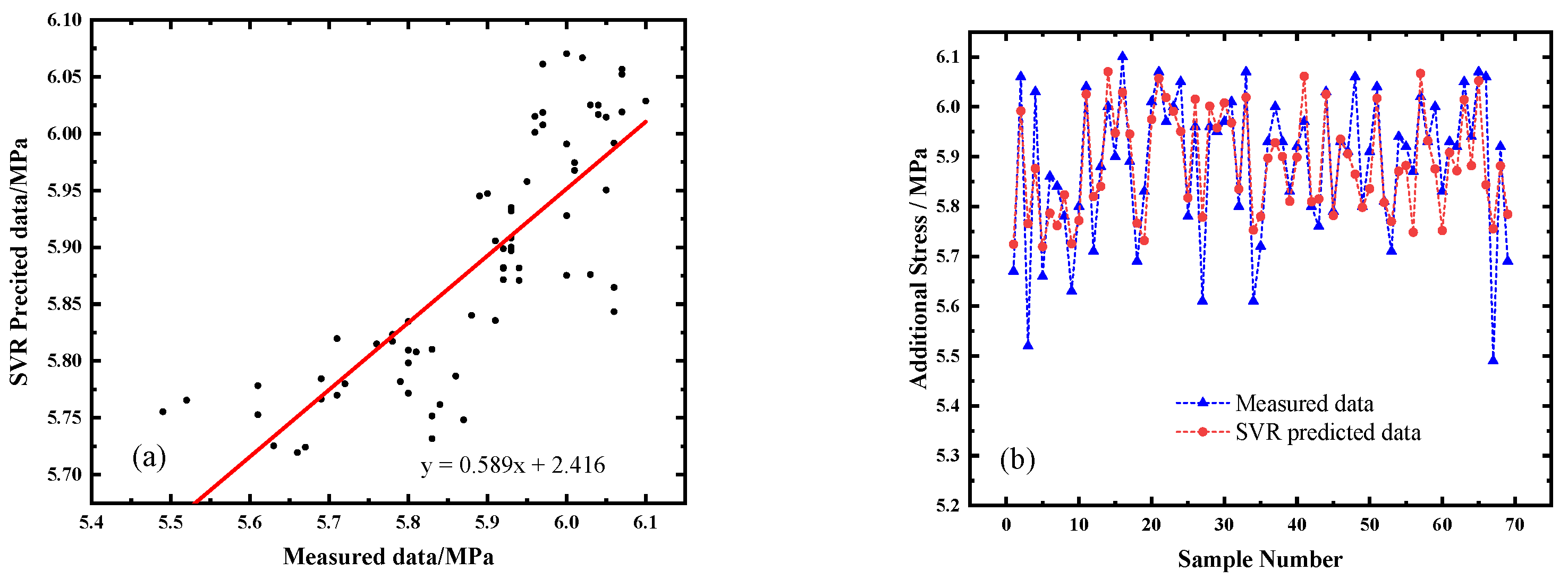
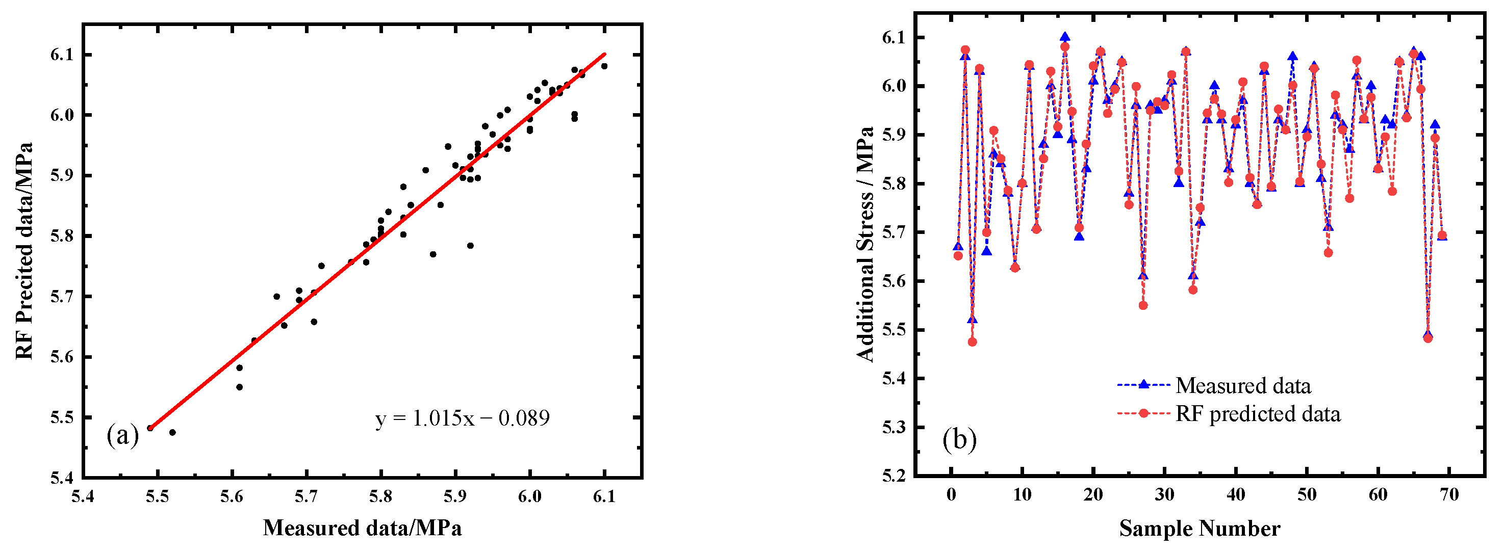
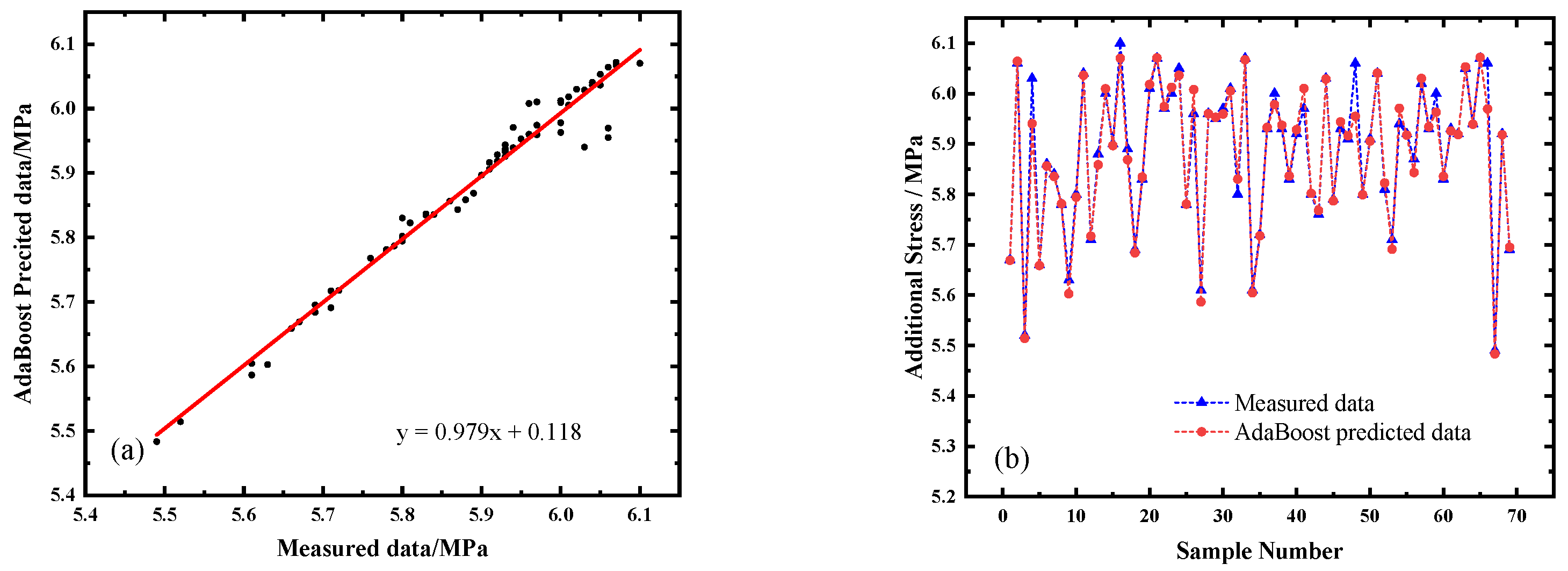
4.2. Comparative Analysis

In the model training process, SVR, along with the other four ensemble-based methods (RF, AdaBoost, GBRT, XGBoost) are validated with the field monitoring data, the results with three performance metrics were presented in

Table 2. Performance comparison of five regression models.

Model Type	Data-Driven Models	RMSE	MAE	${\mathit{R}}^2$
Individual	SVR	0.0910	0.0666	0.6233
Ensemble	RF	0.0288	0.0193	0.9623
	AdaBoost	0.0217	0.0119	0.9758
	GBRT	0.0198	0.0147	0.9821
	XGBoost	0.0154	0.0118	0.9893

. The results are calculated using the test dataset (20% of the whole sample set). Remarkably, all the proposed ensemble models produced satisfactory predictions, showing that XGBoost had the best performance, with RMSE of 0.0154, MAE of 0.0118, and the highest $R^2$ of 0.9893. The predicted results of the RF model were not as accurate as the outputs from other ensemble models, with RMSE of 0.0288 and MAE of 0.0193. In addition, AdaBoost and GBRT models obtained comparable performance, whereas GBRT shows slightly better results in RMSE and $R^2$ metrics. On the contrary, the individual model SVR obtain unacceptable prediction results.

The additional stress prediction details for each model is visualized in Figure 5, Figure 6, Figure 7, Figure 8 and Figure 9. The abscissa of the scatter plot represents the actual monitored value and the ordinate represents the model predicted value. To quantify the fitted relationship between the measured and predicted value, a linear fit is shown in each figure. The most perfect fit is that the measured value is equal to the predicted value, expressed as y = x. That is, the closer the black dots to line y = x, the better the prediction effect. It can be seen from Figure 5a that the results from SVR are quite different from the true data. Figure 6a shows the ensembled model outperforms the individual model, but the RF model for additional stress prediction is not accurate enough. From Figure 7a and Figure 8a, satisfied prediction data are obtained, and most of the data are close to the monitored value. As shown in Figure 9a, XGBoost performs the best agreement between the predicted results and the measured data, with a linear fit equation of y = 0.991x + 0.055. The standard deviation of the predicted points is 0.142.

As the black dots in the scatter plots combined the true value and predicted value, each test sample and its corresponding predicted data are also compared. Figure 5b presents the predicted additional stress of the SVR model differs a lot from the true value, showing that the prediction accuracy is low. As observed in Figure 6b, Figure 7b and Figure 8b, the prediction accuracy of the ensembled model is improved. Although there is a noticeable error between the actual and predicted results at some testing sample points. Regarding the best results, Figure 9b shows that almost all the prediction values of additional stress are closer to the actual value.

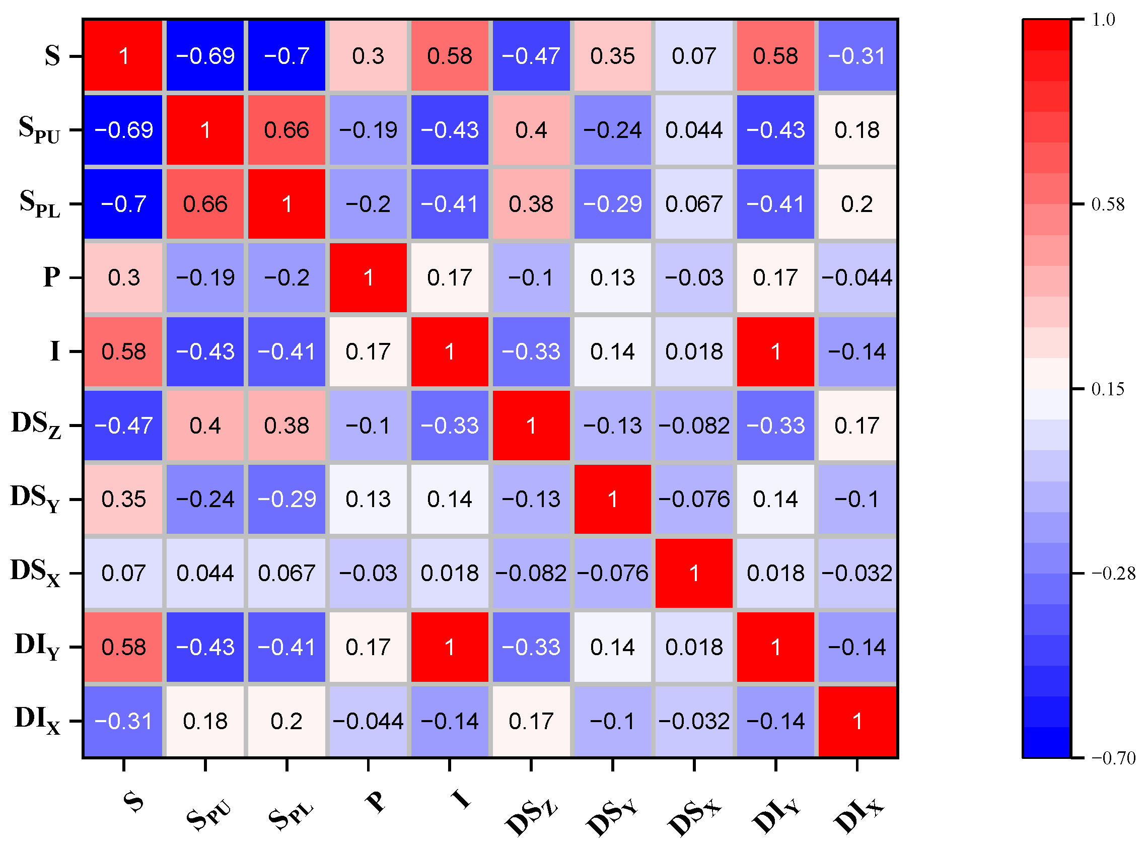
4.3. Sensitivity Analysis

In the prediction models, the relationship between the input variables and the target output has been quantified. To illustrate the importance of the landslide features on the additional stress determination, the importance analysis is conducted for the explanation. The influence of each characteristic on the final predicted additional stress was calculated based on the XGBoost model due to its high performance.

The results were ranked in

Table 3. Feature importance analysis.

Rank (XGBoost)	Monitoring Parameter	Feature Importance (XGBoost)	Rank (RF)	Monitoring Parameter	Feature Importance (RF)
1	Compressive stress	0.5070	1	Compressive stress	0.4109
2	Traction stress	0.2406	2	Traction stress	0.3867
3	Surface y-axis displacement	0.0910	3	Surface y-axis displacement	0.1361
4	Soil pressure	0.0844	4	Inclination	0.0266
5	Surface z-axis displacement	0.0450	5	Soil pressure	0.0249
6	Inclination	0.0162	6	Surface z-axis displacement	0.0081
7	Surface x-axis displacement	0.0119	7	Surface x-axis displacement	0.0055
8	Inner x-axis displacement	0.0039	8	Inner x-axis displacement	0.0010

. The greater the influence on the model prediction, the more significant the feature is. According to the obtained results, compressive stress is listed as the most important feature with feature importance of 0.5070, followed by traction stress with 0.2406. The surface y-axis displacement and soil pressure are the third and fourth most important features, with relative relevance of 0.0910 and 0.0844, respectively. The top four parameters account for more than 90% importance of all of the input variables. It can be seen that the surface z-axis displacement showed 0.045 importance. Moreover, little difference in importance can be found in the inclination and surface x-axis displacement, weighted for 0.0162 and 0.0119, while the inner x-axis displacement indicated the lowest importance. It can be seen from the feature importance of the RF model that the top three factors are the same with XGBoost. Although the importance values vary, rankings other than the inclination factor remain constant for both models.

According to the obtained importance results, the stress plays a more significant role than the displacement, whereas the landslide surface displacement matters a lot more than the inner displacement. The results indicated that the pipe behavior was affected by soil-pipe interaction, and ground movements are consistent with the findings in [35]. Mitigation alternatives can be determined according to the importance of different external influencing factors. However, as the results of machine learning models are closely related to the training data [36], the obtained results are subject to change if a larger database that includes more information and data variability is used since the current database is limited.

5. Conclusions

For the safe service of oil and gas pipelines that cross mountainous areas subject to landslide geohazard, a multi-parameter integrated monitoring system was developed. The joint monitoring for pipeline landslide hazards not only obtains the stress state information of the pipeline, but also the landslide displacement information. To tackle with the interference of invalid measurement data for pipeline stress-strain monitoring, advanced data-driven technologies including SVR, RF, AdaBoost, GBRT, and XGBoost are employed for the prediction of additional stress. Based on the field monitoring data, the relation between landslide movement and pipeline additional stress has been reasonably quantified. From this work, some conclusions are obtained:

• The results indicate that the XGBoost model has the highest performance in the prediction of the additional stress, with RMSE of 0.0154 MPa, MAE of 0.0118 MPa, and $R^2$ value of 0.9893.
• The top five factors contributing to the additional stress for the applied dataset are landslide compressive stress, landslide traction stress, landslide surface y-axis displacement, soil pressure, and landslide surface x-axis displacement.

For further development, the accuracy of the additional stress prediction from the landslide monitoring system can be improved with more monitoring data collected. Overall, the developed technique has allowed the implementation of preventive geotechnical works before a geohazard develops dramatically. In this sense, the model can be seen as a valuable tool that complements existing methodologies and can provide useful information to support the decision-making process.

References

1. Badida, P.; Balasubramaniam, Y.; Jayaprakash, J. Risk evaluation of oil and natural gas pipelines due to natural hazards using fuzzy fault tree analysis. J. Nat. Gas Sci. Eng. 2019, 66, 284–292. [Google Scholar] [CrossRef]
2. Zhang, S.-Z.; Li, S.-Y.; Chen, S.-N.; Wu, Z.-Z.; Wang, R.-J.; Duo, Y.-Q. Stress analysis on large-diameter buried gas pipelines under catastrophic landslides. Pet. Sci. 2017, 14, 579–585. [Google Scholar] [CrossRef]
3. Pu, H.; Xie, J.; Schonfeld, P.; Song, T.; Li, W.; Wang, J.; Hu, J. Railway alignment optimization in mountainous regions considering spatial geological hazards: A sustainable safety perspective. Sustainability 2021, 13, 1661. [Google Scholar] [CrossRef]
4. Teng, M.-C.; Ke, S.-S. Disaster impact assessment of the underground hazardous materials pipeline. J. Loss Prev. Process. Ind. 2021, 71, 104486. [Google Scholar] [CrossRef]
5. Zahid, U.; Godio, A.; Mauro, S. An analytical procedure for modelling pipeline-landslide interaction in gas pipelines. J. Nat. Gas Sci. Eng. 2020, 81, 103474. [Google Scholar] [CrossRef]
6. Yavorskyi, A.; Karpash, M.; Zhovtulia, L.; Poberezhny, L.Y.; Maruschak, P. Safe operation of engineering structures in the oil and gas industry. J. Nat. Gas Sci. Eng. 2017, 46, 289–295. [Google Scholar] [CrossRef]
7. Zheng, J.; Zhang, B.; Liu, P.; Wu, L. Failure analysis and safety evaluation of buried pipeline due to deflection of landslide process. Eng. Fail. Anal. 2012, 25, 156–168. [Google Scholar] [CrossRef]
8. Vasseghi, A.; Haghshenas, E.; Soroushian, A.; Rakhshandeh, M. Failure analysis of a natural gas pipeline subjected to landslide. Eng. Fail. Anal. 2021, 119, 105009. [Google Scholar] [CrossRef]
9. Ali, H.; Choi, J.-H. A review of underground pipeline leakage and sinkhole monitoring methods based on wireless sensor networking. Sustainability 2019, 11, 4007. [Google Scholar] [CrossRef]
10. Guo, W.; Liu, Y.; Li, C. Stress analysis and mitigation measures for floating pipeline. IOP Conf. Ser. Earth Environ. Sci. 2017, 59, 012014. [Google Scholar] [CrossRef] [Green Version]
11. Xu, P.; Zhang, M.; Lin, Z.; Cao, Z.; Chang, X. Additional stress on a buried pipeline under the influence of coal mining subsidence. Adv. Civ. Eng. 2018, 2018, 3245624. [Google Scholar] [CrossRef]
12. Zhang, S.; Liu, B.; He, J. Pipeline deformation monitoring using distributed fiber optical sensor. Measurement 2019, 133, 208–213. [Google Scholar] [CrossRef]
13. Yin, J.; Li, Z.-W.; Liu, Y.; Liu, K.; Chen, J.-S.; Xie, T.; Zhang, S.-S.; Wang, Z.; Jia, L.-X.; Zhang, C.-C.; et al. Toward establishing a multiparameter approach for monitoring pipeline geohazards via accompanying telecommunications dark fiber. Opt. Fiber Technol. 2022, 68, 102765. [Google Scholar] [CrossRef]
14. Li, X.; Wu, Q.; Jin, H.; Kan, W. A new stress monitoring method for mechanical state of buried steel pipelines under geological hazards. Adv. Mater. Sci. Eng. 2022, 2022, 4498458. [Google Scholar] [CrossRef]
15. Sarvanis, G.C.; Karamanos, S.A. Analytical model for the strain analysis of continuous buried pipelines in geohazard areas. Eng. Struct. 2017, 152, 57–69. [Google Scholar] [CrossRef]
16. Xin, L.; Mingzhou, B.; Bohu, H.; Pengxiang, L.; Lebin, Z.; Yun, C.; Hai, S. Safety analysis of landslide in pipeline area through field monitoring. J. Test. Eval. 2021, 51, e200751. [Google Scholar] [CrossRef]
17. Xu, W.; Xu, H.; Chen, J.; Kang, Y.; Pu, Y.; Ye, Y.; Tong, J. Combining numerical simulation and deep learning for landslide displacement prediction: An attempt to expand the deep learning dataset. Sustainability 2022, 14, 6908. [Google Scholar] [CrossRef]
18. Yan, Y.; Yang, D.-S.; Geng, D.-X.; Hu, S.; Wang, Z.-A.; Hu, W.; Yin, S.-Y. Disaster reduction stick equipment: A method for monitoring and early warning of pipeline-landslide hazards. J. Mt. Sci. 2019, 16, 2687–2700. [Google Scholar] [CrossRef]
19. Kunert, H.G.; Otegui, J.; Marquez, A. Nonlinear fem strategies for modeling pipe–soil interaction. Eng. Fail. Anal. 2012, 24, 46–56. [Google Scholar] [CrossRef]
20. Wei, A.; Yu, K.; Dai, F.; Gu, F.; Zhang, W.; Liu, Y. Application of tree-based ensemble models to landslide susceptibility mapping: A comparative study. Sustainability 2022, 14, 6330. [Google Scholar] [CrossRef]
21. Alvarado-Franco, J.P.; Castro, D.; Estrada, N.; Caicedo, B.; Sánchez-Silva, M.; Camacho, L.A.; Muñoz, F. Quantitative-mechanistic model for assessing landslide probability and pipeline failure probability due to landslides. Eng. Geol. 2017, 222, 212–224. [Google Scholar] [CrossRef]
22. Liu, S.; Wang, H.; Li, R.; Ji, B. A novel feature identification method of pipeline in-line inspected bending strain based on optimized deep belief network model. Energies 2022, 15, 1586. [Google Scholar] [CrossRef]
23. Yan, Y.; Xiong, G.; Zhou, J.; Wang, R.; Huang, W.; Yang, M.; Wang, R.; Geng, D. A whole process risk management system for the monitoring and early warning of slope hazards affecting gas and oil pipelines. Front. Earth Sci. 2022, 9, 812527. [Google Scholar] [CrossRef]
24. Ding, Y.; Yang, H.; Xu, P.; Zhang, M.; Hou, Z. Coupling interaction of surrounding soil-buried pipeline and additional stress in subsidence soil. Geofluids 2021, 2021, 7941989. [Google Scholar] [CrossRef]
25. Radwan, A.E.; Wood, D.A.; Radwan, A.A. Machine learning and data-driven prediction of pore pressure from geophysical logs: A case study for the mangahewa gas field, new zealand. J. Rock Mech. Geotech. Eng. 2022. [Google Scholar] [CrossRef]
26. Awad, M.; Khanna, R. Support vector regression. In Efficient Learning Machines; Springer: Berlin/Heidelberg, Germany, 2015; pp. 67–80. [Google Scholar]
27. Jia, Z.; Ho, S.-C.; Li, Y.; Kong, B.; Hou, Q. Multipoint hoop strain measurement based pipeline leakage localization with an optimized support vector regression approach. J. Loss Prev. Process. Ind. 2019, 62, 103926. [Google Scholar] [CrossRef]
28. Rodriguez-Galiano, V.; Sanchez-Castillo, M.; Chica-Olmo, M.; Chica-Rivas, M. Machine learning predictive models for mineral prospectivity: An evaluation of neural networks, random forest, regression trees and support vector machines. Ore Geol. Rev. 2015, 71, 804–818. [Google Scholar] [CrossRef]
29. Roy, M.-H.; Larocque, D. Robustness of random forests for regression. J. Nonparametr. Stat. 2012, 24, 993–1006. [Google Scholar] [CrossRef]
30. Ying, C.; Qi-Guang, M.; Jia-Chen, L.; Lin, G. Advance and prospects of adaboost algorithm. Acta Autom. Sin. 2013, 39, 745–758. [Google Scholar]
31. Riccardi, A.; Fernández-Navarro, F.; Carloni, S. Cost-sensitive adaboost algorithm for ordinal regression based on extreme learning machine. IEEE Trans. Cybern. 2014, 44, 1898–1909. [Google Scholar] [CrossRef]
32. Huang, Y.; Liu, Y.; Li, C.; Wang, C. Gbrtvis: Online analysis of gradient boosting regression tree. J. Vis. 2019, 22, 125–140. [Google Scholar] [CrossRef]
33. Nie, P.; Roccotelli, M.; Fanti, M.P.; Ming, Z.; Li, Z. Prediction of home energy consumption based on gradient boosting regression tree. Energy Rep. 2021, 7, 1246–1255. [Google Scholar] [CrossRef]
34. Chen, T.; Guestrin, C. Xgboost: A scalable tree boosting system. In Proceedings of the 22nd ACM SIGKDD International Conference on Knowledge Discovery and Data Mining, San Francisco, CA, USA, 13–17 August 2016; pp. 785–794. [Google Scholar]
35. Ferreira, N.J.; Blatz, J.A. Measured pipe stresses on gas pipelines in landslide areas. Can. Geotech. J. 2021, 99, 1855–1869. [Google Scholar] [CrossRef]
36. Liu, Y.; Bao, Y. Review on automated condition assessment of pipelines with machine learning. Adv. Eng. Inform. 2022, 53, 101687. [Google Scholar] [CrossRef]
Figure 1. Schematic diagram of the evolution of pipeline geological hazards.
Sustainability 14 11999 g001
Figure 2. Schematic of the landslide monitoring system.
Sustainability 14 11999 g002
Figure 3. Flowchart of the proposed approach.
Sustainability 14 11999 g003
Figure 4. Correlation matrix of every two attributes.
Sustainability 14 11999 g004
Figure 5. Predicted results of SVR. (a) Scatter plots of the predicted versus measured data. (b) Comparison of predicted and measured data.
Sustainability 14 11999 g005
Figure 6. Predicted results of RF. (a) Scatter plots of the predicted versus measured data. (b) Comparison of predicted and measured data.
Sustainability 14 11999 g006
Figure 7. Predicted results of AdaBoost. (a) Scatter plots of the predicted versus measured data. (b) Comparison of predicted and measured data.
Sustainability 14 11999 g007
Figure 8. Predicted results of GBRT. (a) Scatter plots of the predicted versus measured data. (b) Comparison of predicted and measured data.
Sustainability 14 11999 g008
Figure 9. Predicted results of XGBoost. (a) Scatter plots of the predicted versus measured data. (b) Comparison of predicted and measured data.
Sustainability 14 11999 g009