Article

Prediction of Spatial Likelihood of Shallow Landslide Using GIS-Based Machine Learning in Awgu, Southeast/Nigeria

by
Uzodigwe Emmanuel Nnanwuba
1,
Shengwu Qin
1,*,
Oluwafemi Adewole Adeyeye
2,
Ndichie Chinemelu Cosmas
3,
Jingyu Yao
1,
Shuangshuang Qiao
1,
Sun Jingbo
1 and
Ekene Mathew Egwuonwu
1
1
College of Construction Engineering, Jilin University, Changchun 130026, China
2
College of New Energy and Environment, Jilin University, Changchun 130021, China
3
Department of Geography, University of Nigeria, Nsukka 410001, Nigeria
*
Author to whom correspondence should be addressed.
Sustainability 2022, 14(19), 12000; https://doi.org/10.3390/su141912000
Submission received: 4 May 2022 / Revised: 9 July 2022 / Accepted: 7 September 2022 / Published: 22 September 2022

Abstract

:
A landslide is a typical geomorphological phenomenon associated with the regular cycles of erosion in tropical climates occurring in hilly and mountainous terrain. Awgu, Southeast Nigeria, has suffered a severe landslide disaster, and no one has studied the landslide susceptibility in the study area using an advanced model. This study evaluated and compared the application of three machine learning algorithms, namely, extreme gradient boosting (Xgboost), Random Forest (RF), and Naïve Bayes (NB), for a landslide susceptibility assessment in Awgu, Southeast Nigeria. A hazard assessment was conducted through a field investigation, remote sensing, and a consultation of past literature reviews, and 56 previous landslide locations were prepared from various data sources. A total of 10 conditioning factors were extracted from various databases and converted into a raster. Before modeling the landslide susceptibility, the information gain ratio (IGR) was used to select and quantitatively describe the predictive ability of the conditioning factors. The Pearson correlation coefficient was used to judge the correlation between 10 conditioning factors. In this study, rainfall is the most significant factor with respect to landslide distribution and occurrence. The confusion matrix, the area under the receiver operating characteristic curve (AUROC), was used to validate and compare the models. According to the AUROC results, the prediction accuracy for the RF, NB, and XGBOOST models are 0.918, 0.916, and 0.902, respectively. This current study can support the landslide susceptibility assessment of Awgu, Southeast Nigeria, and can provide a reference for other areas with the same conditions.

1. Introduction

Landslides are among the critical natural hazards that have seriously impacted the landscape and that increasingly threaten the lives and resources of society in Enugu State, Nigeria [1]. Furthermore, landslides cause a loss of fertile soil and land degradation [2]. In southeastern Nigeria, especially in Enugu state, the leading causes of landslides are the nature of the slope, the soil properties, and the torrential rains, which are complex processes that lead to the rapid development of landslides of different sizes [1]. In Awgu, landslide activities are being reported in the failed escarpment within the northwest-trending ridge [3]. Over the last few decades, there has been an increased recognition that more attention needs to be paid to hilly terrains and mountainous regions because of their diverse, fragile geomorphic systems and continuous changes occurring at spatial and temporal scales [4,5]. Hence, there is a need for regular and continuous landslide-monitoring information to reduce the damage of landslides to humans and their possessions [6]. A landslide susceptibility map (LSM) is widely accepted as a standard tool to delineate region prone to landslide and the first step in reducing the risk of landslide disasters [7,8]. The map also enables the creation of a model that can be used for optimal land use planning to avoid landslides [9].
The approaches of landslide susceptibility studies can be categorized as qualitative and quantitative. The qualitative approach relies on determining the landslide susceptibility related to data recognition and subjective in nature that requires a geological expert knowledge [10,11]. On the other hand, the quantitative approach employs the estimation of numerical values using a probabilistic statistical method based on the objective of the mathematical structure of the spatial distribution of landslide occurrences and the influencing factors [12]. The rapid increase in geospatial technology and geo-computing methods has given rise to the popularity of the qualitative approach because it provides more accurate results [13]. The most commonly used qualitative methods for landslide susceptibility maps are the frequency ratio [14], the analytic hierarchy process [15], the weight of evidence [11], and logistic regression [16]. The qualitative and quantitative approaches’ limitations vary in terms of accuracy, repeatability, and time scale [17]. To bridge this knowledgeable gap, recent landslide studies using remote-sensing data and GIS-based machine learning algorithms for landslide susceptibility modeling have yielded high accuracy results and LSM [18,19]. In landslide studies, the advantage of machine learning models is based not only on the ease of addressing misclassification issues but also on their usefulness in inaccessible areas and for making a prediction based on the relationship between events and their drivers [20,21]. Some examples of machine learning methods that have been used in the landslide literature are the support vector machine (SVM) [22], artificial neural network (ANN) [23,24], decision table (DT) [25], credal decision tree (CDT) [26], extreme gradient boosting (XGBOOST) [27,28], adaptive neuro-fuzzy inference system (ANFIS) [29,30], random forest (RF) [21,31,32], Naive Bayes (NB) [33,34], and reduced error pruning tree (REPTree) [35].
Landslides are profound reoccurring hazards in the southeastern region of Nigeria, where landslide occurrences date back to 1970. There is a need to identify and map landslide-prone areas to serve as a support system for land planners and decision makers and educate locals on the ways to achieve landslide mitigation in the region using more robust and reliable technological measures. It is on this initial premise that we employ XGBOOST, RF, and NB machine learning algorithms in Awgu, southeast Nigeria, to produce a landslide susceptibility map with the potential of explaining the intricate relationship between environmental predictors and responses. XGBoost has been applied in different parts of the world and has been confirmed as outstanding with respect to susceptibility models [28,36,37]. RF is a vital machine learning model that can handle high data dimensionality and multicollinearity and efficiently classify datasets in remote sensing and landslide susceptibility mapping [2,38,39]. NB is a fast, supervised classification method suitable for large-scale predictions and the classification of complex and incomplete datasets [40]. Although XGBOOST, RF, and NB models have been used for landslide susceptibility mapping in different parts of the world and have been found to be effective, there is a paucity of applications and comparisons of these models for landslide assessments in Nigeria. The output of this study will assist land planners and decision makers and add to the reliable landslide literature in Nigeria.

2. Study Area

The Awgu local government area, a part of Enugu State, Nigeria, occupies an area of about 449.53 km2, and it is located between the latitude of 06.00° N and 06.19° N and the longitude of 07.23° E and 07.35° E. The area is bounded by five local government areas: Nkanu West, Nkanu East, Aninri, Udi, the Oji River, and Abia State to the south (Figure 1).
The topography is dominated by the slightly NE–SW trending escarpment that transverses the area with its highest elevation at 505 m above sea level and its approximate lowest elevation at 69 m above sea level (Figure 1). Awgu generally has two tropical periods: a period of rainfall (wet season) and a dry season. The rainy season begins in April and ends in October [3], while the dry season runs from October to March. The annual temperature of the area ranges from 27 °C to 28 °C, and the stability of the slopes is adversely affected by both the rainy and dry seasons because of the characteristic components of the rock types. Throughout the region, the geology includes the Asu River group (32.71%), Asata shale group (4.57%), Awgu Ndeaboh shale group (7.24%), Eze Aku shale group (8.15%), lower coal measures (24.45%), and upper coal measures (22.88%). The land use/land cover varieties present in the area are built-up (8.89%), bare land (20.24%), vegetation (37.77%), rocky outcrop (21.92%), and farmland (11.18%). The vegetation of the region belongs to the Guinea savannah consisting of grass interspersed with shrubs and medium-sized trees. The region’s initiation and the mobility of several landslides are attributed to the dominant formations caused by heavy rainfall and human activities, which are destroying farmland.

3. Materials and Methods

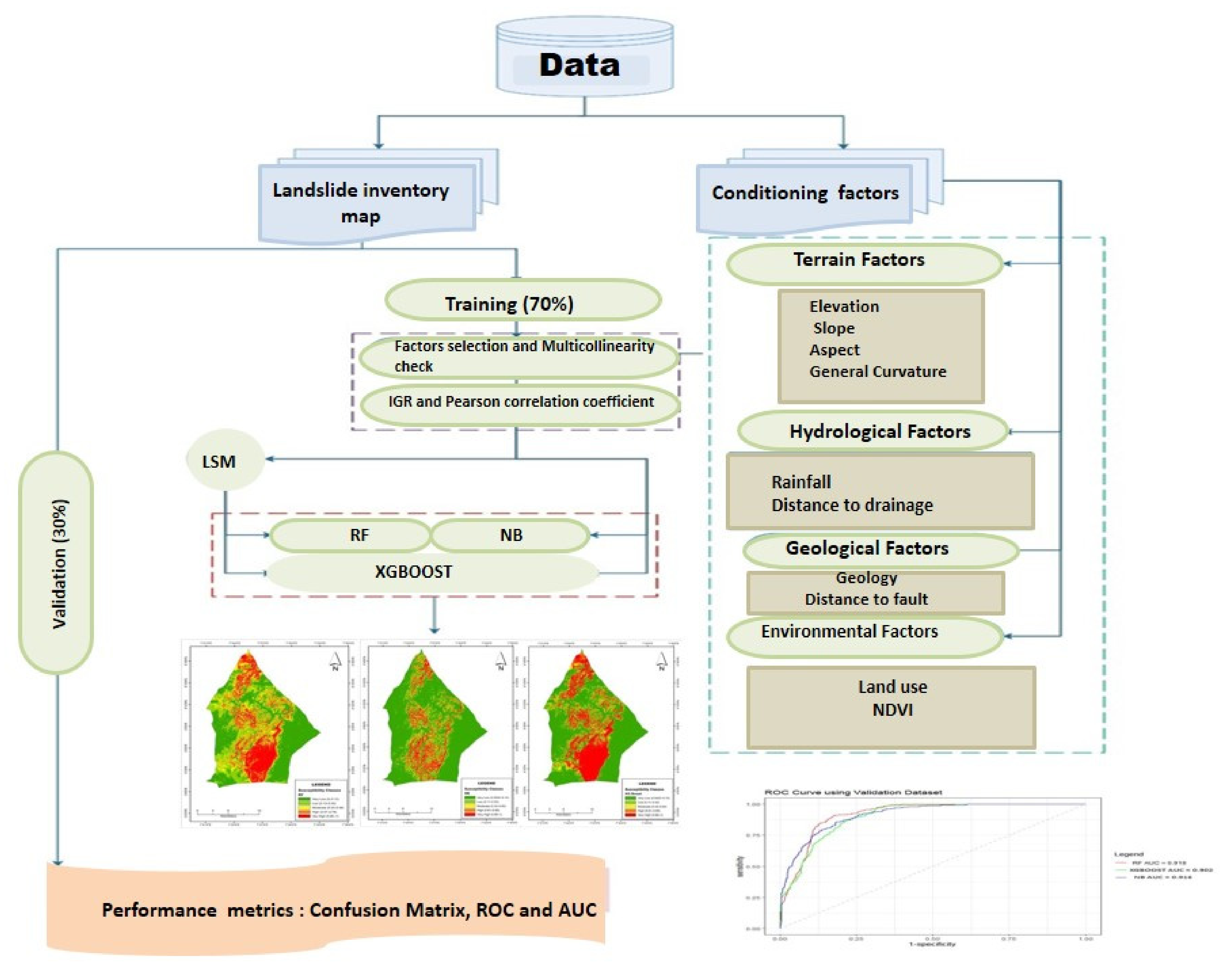
The methodology of this study is built from two stages: secondary and primary research. Secondary research was undertaken such that before developing the research methodology, a detailed literature review was performed on local and global research into landslide susceptibility and its impact on the environment, as mentioned earlier in Section 1. Secondary research data involved consulting geological maps, meteorological maps, DEM, historical reports on previously measured data on landslide inventories and distribution, topographic maps, and Landsat 8 OLI images. A geological map of 1:250,000 was obtained from the Department of Geography, University of Nigeria, Nsukka.Landsat 8 OLI images were downloaded from the United States Geological Survey center (http://earthexplorer.usgs.gov/, accessed on 7 June 2020). The annual rainfall records of the study area from 2011 to 2020 were downloaded from (http://www.cru.uea.ac.uk, accessed on 21 March 2021). Higher resolution elevation is required to study the details of shallow landslides [41]. Therefore, a SRTM-DEM with a high resolution of 30 m × 30 m was extracted from the google earth engine. Four other conditioning factors were extracted from the digital elevation model for the essential preparations of the landslide susceptibility map (LSM). Primary research in the study area involved fieldwork to delineate the past historical landslide areas using GPS and checking the landslide areas using remote sensing (Google Earth) and GIS. The roadmap to the successful completion of this methodology includes:
  • Preparation of landslide inventory map and conditioning factors.
  • The selection of conditioning factors, which was performed using the information gain ratio. The Pearson correlation coefficient was employed to judge the correlation between conditioning factors prior to landslide susceptibility modeling.
  • Preparation of landslide susceptibility modeling using Random Forest, Naive Bayes, and XGBOOST algorithms.
  • The use of a confusion matrix, receiver operating characteristic curve, and the area under the curve to evaluate the models (Figure 2).

3.1. The Preparation of Landslide Inventory Map

The landslide inventory map is essential for predicting future landslides [42]. It contains vital and indispensable information for the spatial forecasting of landslides. In the current study, a comprehensive field survey and previously measured data of past landslide records from 2008 to 2011 accounted for 56 of the landslide locations that were observed and verified on a scale map of 1:50,000. Selecting an appropriate mapping unit is critical to assessing landslide susceptibility. Thus, the grid unit mapping approach was employed because it is widely used for mapping landslide susceptibility and has the advantage of a regular shape suitable for fast subdivision and high model efficiency [43]. The 56 landslide locations were represented as a polygonal dataset and imported into QGIS, where the automatic extraction of the grid units of the study area was performed using a user-friendly automatic extraction tool pack called LaGriSU [44]. Details on the landslide sample and non-landslide sample extractions using LaGriSU are discussed in Section 5.1.
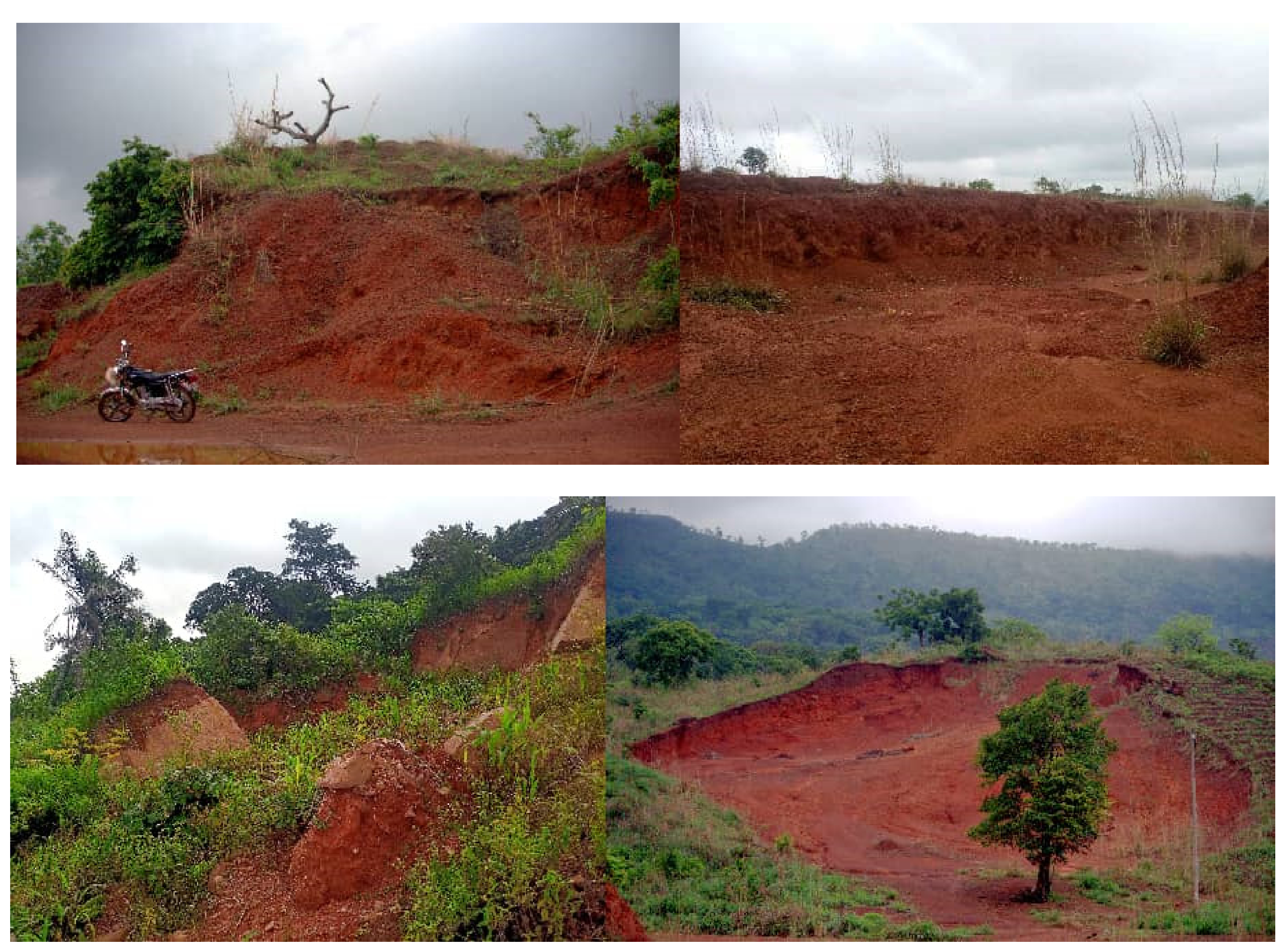
Furthermore, the predominant type of landslide in this region is rock wall or rock falls (30.36%), debris slides (17.86%), and soil slides (51.78%) [3]. The total area covered by landslides in the study area is 522,051.482 m2. The smallest landslide was 831.31 m2, and the largest was 60,925.02 m2. The mean size of the landslide was 9322.35 m2. Pictures of landslides taken in the study area is shown in (Figure 3).

3.2. Conditioning Factor Selection and Multicollinearity Check

In the context of landslide assessment, the conditioning factor’s role is to represent a region’s environmental information [45]. Therefore, it is necessary to check and exclude factors that may introduce noise during the modeling of landslide susceptibility, resulting in the degradation of the model’s predictive performance [46]. Information gain ratio was used to select and quantitatively describe the predictive ability of each of the conditioning factors, and the Pearson correlation coefficient was used to judge the correlation between each conditioning factor [45].
Information gain ratio means the ratio of information gained to intrinsic information [47]. It also helps determine the importance of each factor for modeling; thus, it suggests the appropriate weights to assign to each factor when generated [19]. The higher the information gain ratio value, the greater the importance of the conditioning factors [48]. The formula used for calculating the information gain ratio is given below [45,49]:
H D = i = 1 n D i D log 2 D i D
IG D , A = H D H D | A
IGR D , A = IG D , A H A D
For the sample set, the probability of each category is D i D , where D i represents the number of samples for the category, and D represents the total number of samples. Otherwise, the current characteristic A is treated as a random variable for calculating empirical entropy   H A D . Pearson correlation coefficient is a combination of the strength and direction of the relationship of variables. It ranges from −1 to 1 in value, where −1 indicates the strongest inverse correlation, and +1 indicates a strong correlation of variables. It is highly correlated if the value is >0.7 [50]. The formula for the Pearson correlation coefficient used in this study is the same as the formula used by [49] and is given as follows:
r = i = 1 n X i X ¯ Y i Y ¯ i = 1 n X i X ¯ 2 i = 1 n Y i Y ¯ 2
where n is the number of testing samples, and X i and Y i represent the observed values of point i corresponding to variables X and Y , respectively. In contrast, X ¯ and Y ¯ are defined as the average value of the sample.

3.3. Conditioning Factors (CF)

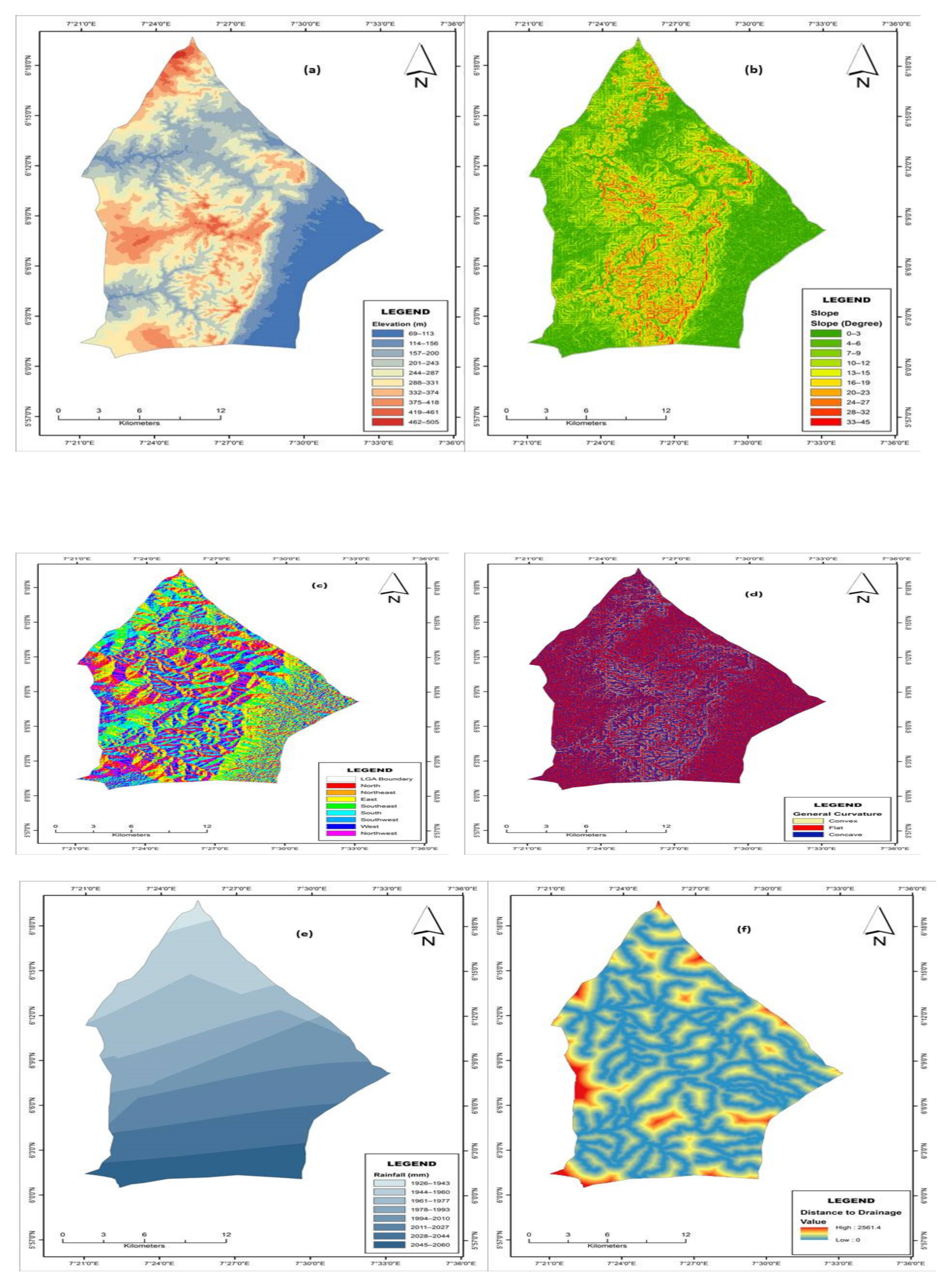
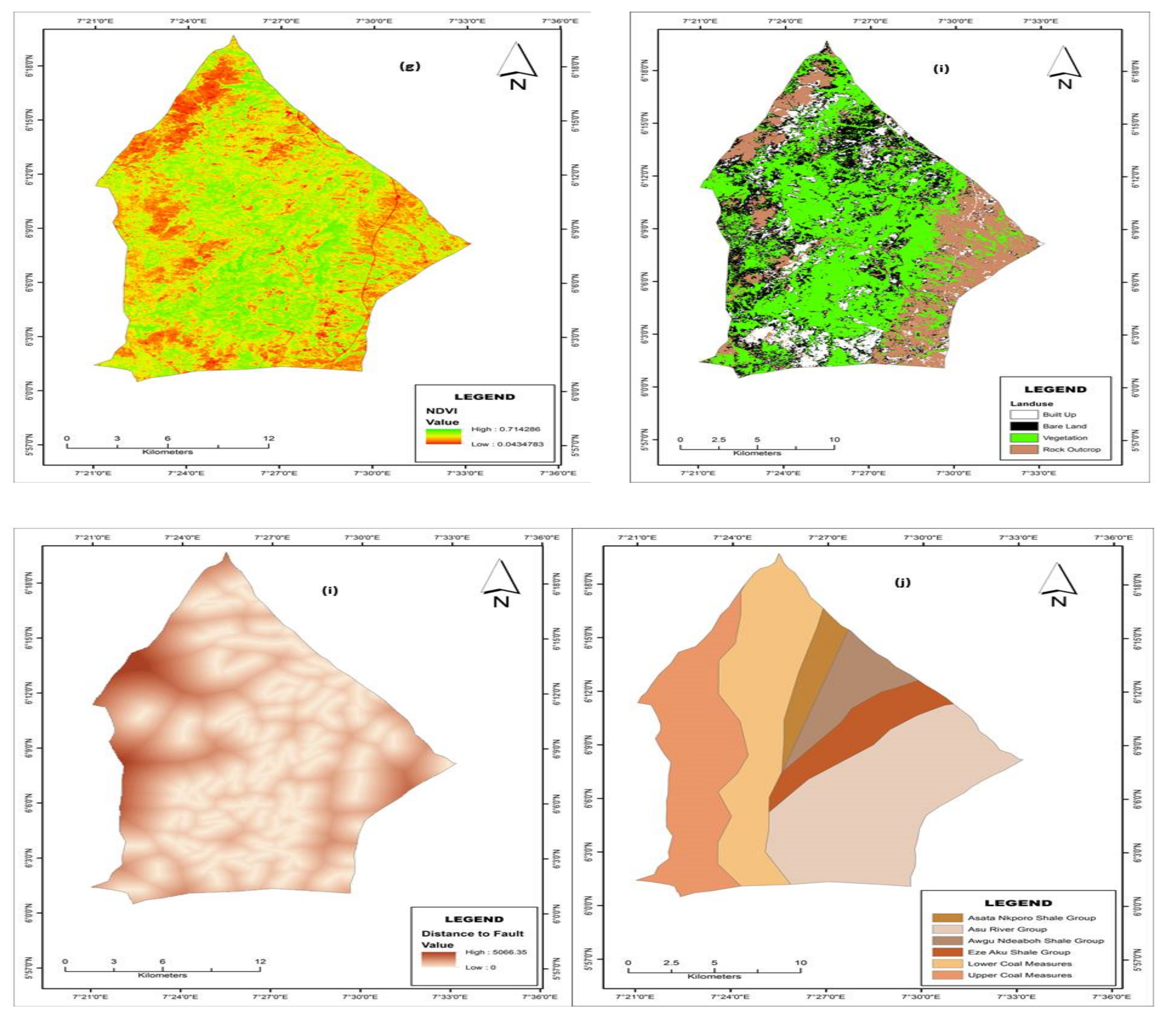
Incorporating appropriate landslide conditioning factors is necessary to use soft computing techniques as a direct method of assessing landslide susceptibility since influential variables help improve the model’s predictive performance [35]. However, after consultation with past literature, selecting the conditioning factors, and due to the nature of the shallow landslide distribution in this study, ten conditioning factors were used for landslide analysis, namely, elevation, slope, aspect, general curvature, rainfall, distance to drainage, NDVI, land use, distance to fault, and geology. Experts confirm the Digital Elevation Model as the primary method used to analyze catchment topography [51]. Due to its topographical effects, it dramatically affects precipitation and vegetation [41]. The slope is a significant factor in susceptibility studies because it has been confirmed that landslide incidence varies with different structures [52]. Slope affects the magnitude of both standard and shear stresses on the potential surface of failures [53]. Where the slope is high in a region, creep landslide can occur depending on the surface erosion and drainage. The slope map (Figure 4b) was produced from the elevation using the GDAL tools in QGIS. Aspect is a significant factor that shows the direction of the maximum slope. It is associated with rainfall, wind direction, weathering, and sunshine duration [54]. Aspect directly affects the occurrences of landslides and indirectly affects the climatic conditions. In this study, the aspect has eight faces (Figure 4c). General Curvature is a significant factor in landslide susceptibility studies since the stability of slopes varies, which makes them very important with respect to landslide occurrence. The curvature of the study was classified into three categories: convex, flat, and concave (Figure 4d). Rainfall has been considered one of the critical triggers inducing landslide factors in the study area [1]. Constant and heavy rainfall can directly lead to a landslide. Zonal interpolation using the inverse distance weight (IDW) technique was performed to obtain the annual rainfall data of Awgu over nine years (2011–2020) (Figure 4e). The stability of slopes is the degree of saturation [55] affected by drainage. Water often modifies the rock mass of the slope, which significantly reduces the shear strength of the rock mass [56]. The elevation map was used to extract the drainage data in this study using SAGA tools in QGIS, and Euclidean distance was calculated in ArcGIS to obtain the distance to the drainage map (Figure 4f). NDVI has been identified as another critical conditioning factor in the spatial distribution of landslides and varies from −1 to 1 [57]. The NDVI map (Figure 4g), concerning five years from 2008–2012, was extracted from the Google Earth Engine. Land use is one of the essential factors of slope stability [58]. The LU/LC was extracted from Landsat 8 OLI images. The land use types of the study area consist of (A) built-up, (B) bare-land, (C) vegetation, and (D) rocky outcrop. (Figure 4j). Faults are responsible for triggering many landslides due to the tectonic breaks that decrease the rock strength [59]. The lineament density map used in this study was obtained from Landsat 8 OLI images using PCI Geomatica 2016 and ArcGIS applications. The lineament density was preprocessed to a mosaic and converted to a composite band using ArcGIS software. The result of the lineament density was converted to a shape file, which was used for density calculation, where the line density tool was used to determine the lineament distribution over the study. The Area and Euclidean distance were obtained using the spatial analyst toolset of ArcGIS. The distance to fault ranges from 0 to 5066.35 m (Figure 4i). Geology is one of the most crucial factors for landslide susceptibility mapping [60]. The geological map of the current study was digitized, and six geological formations were found: Asu river group, Asata Nkporo shale group, Awgu Ndeaboh shale group, Eze Awku shale group, lower coal measures, and upper coal measures (Figure 4).

3.4. Methodology

It is essential to select an appropriate machine learning model for mapping landslide susceptibility [61]. Different models to predict landslide damage can be reduced [20,62]. With respect to predicting landslides, GIS-based machine learning techniques provide knowledge of the landslide-prone area [18]. Based on the scale of the data, the quality of the data, and the spatial distribution of landslides in the study area, three machine learning models were chosen: XGBOOST, RF, and NB. These models were implemented using the classification and regression-training (CARET) package in the R programming language.

3.4.1. Extreme Gradient Boosting (XGBOOST)

XGBoost is an ensemble learner based on a decision tree’s building structure. The authors of [63,64] first introduced extreme gradient boosting, a commonly used machine algorithm to solve all objective functions regarding gradient in imbalanced datasets [65]. The Xgboost model uses many classification and regression trees and combines them using the gradient-boosting method [66]. The primary function of using Xgboost is to predict a new classification membership after each iteration [39]. The main advantage of Xgboost is its integration of various dimensions of datasets to some extent, and those features’ combination contributes primarily to the process of efficiency prediction.

3.4.2. Random Forest (RF)

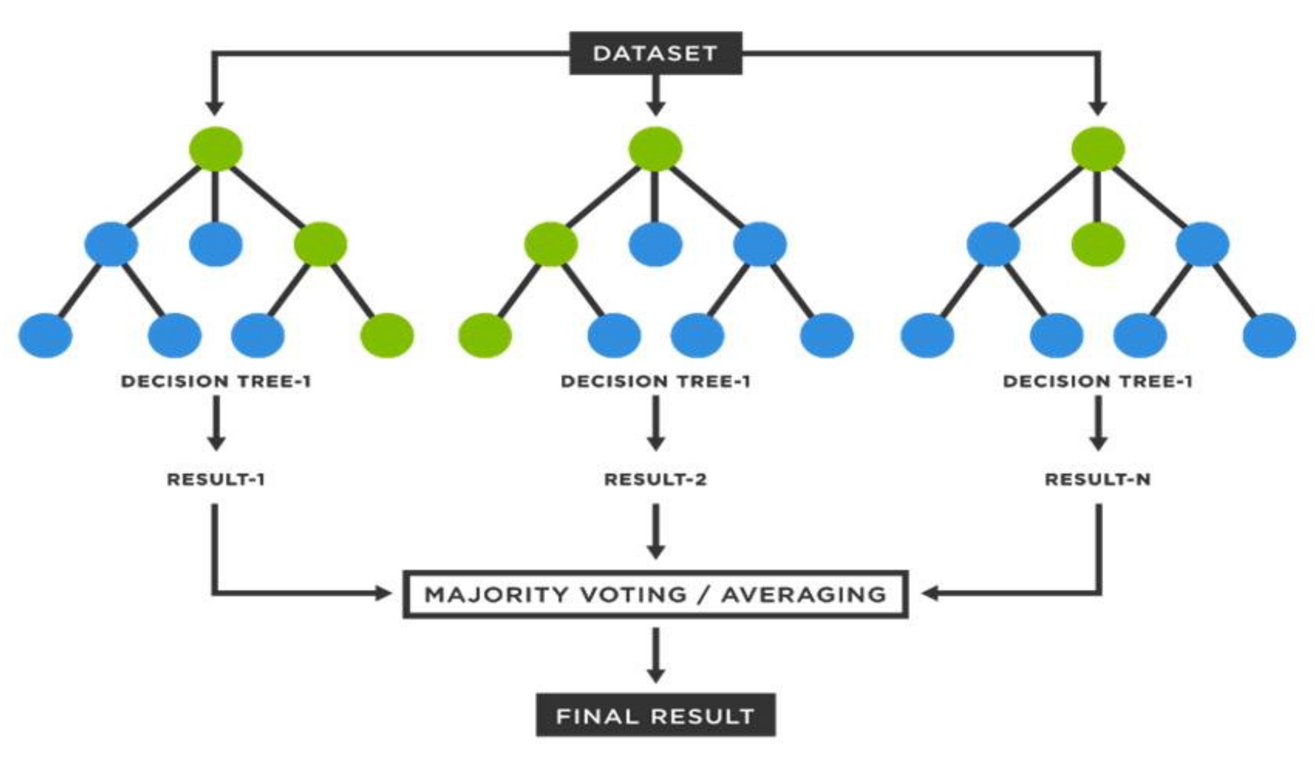
RF modelling is the ensemble of decision trees invented by [67]. RF modelling is based on bagging, which is used to reduce variations in the prediction by combining the result of multiple decision trees on different samples of the dataset. RF modelling needs two parameters to create and generate a classification: (1) the number of trees in the forest (ntree) and (2) the number of variables tested at each node to grow the tree (mtry) [68]. It produces many classification trees, each voting for an input dataset, and the overall voting of the trees produces the output class of the input [69]. During the process, approximately one-third of the instances are dropped from the training set and remain as an out-of-bag sample that can be used to assess the classification accuracy of the trees [70]. The out-of-the-bag (OOB) parameter calculates the model’s error, which is equal to the standard deviation error between predicted values [59]. RF algorithm can be used in the construction of LSM to calculate the importance of geospatial variables [8] and has a precise predictive impact on the spatial likelihood of landslide occurrences. Flowchart of a random forest is shown in (Figure 5).

3.4.3. Naive Bayes

Naïve Bayes (NB) method is a statistical classification approach with no dependency between attributes and that attempts to maximize posterior probability in determining classes [71,72]. NB method is based on the independent hypothesis among predictor variables that affect its predictive accuracy [73]. The Naïve Bayes classifier treats the input features separately in the construction and prediction stages. The application of NB to landslide susceptibility is a relatively robust, reliable for use with low datasets, and non-time-consuming model [34,48]. The NB classifier assumes that the impact of one predictor’s values (X) on a given class (C) is independent of the values of other predictors.
P c | X = P ( x 1 | c ) X   P ( x 2 | c )   X     X   P ( x n | c )   X   P ( c )
where P c | X is the posterior probability class (target) given the predictor (attribute); P ( x 1 | c ,   x 2 | C   x n | c ) is the likelihood, which is the probability of the predictor given the class; and P ( c )   is   the   prior   probability   of   class .

3.5. Hyperparameter Optimization

When mapping landslide susceptibility, The choice of model parameters is a key factor in the model’s accuracy [74]; in machine learning, hyperparameter adjustment (optimization) is required whenever the default settings do not give satisfactory results or take too much time [65]. It is time-consuming to adjust the parameters manually; therefore, in this study, two hyperparameter searches (grid search and random search) were employed to allow the machine to find the best combination for the optimization. RF modelling is simple and requires minimal tweaking [75,76]. The hyperparameter employed for RF modeling tends to have both recommended and default values [66]. The hyperparameter optimization used in the RF modeling is the random search. Xgboost’s performance is controlled by hyperparameter optimization [63]. The hyperparameter of the XGBOOST used was the grid search and the optimization settings were max_depth = 6, min_child = 1, gamma = 0.1, sample = 1, colsample_bytree = 0.75, and eta = 0.05. Furthermore, the grid search of NB model was employed in the current study and optimized with Laplace correction = 0, distribution type = T, and bandwidth adjustment = 1.0. The resampling techniques used a 10-fold cross-validation and repeated this cross-validation 3 times for a random search with the RF model and grid search for both the Xgboost and NB models. For both the Xgboost and NB models, cross-validation was performed 10-fold and was repeated 3 times with each set. Seed (849) was used.

3.6. Performance Metrics

After establishing the machine learning models, the next step is assessing the model capability. The confusion matrix consists of a (2 by 2) contingency table that contains four types of possible outcomes (TP, TN, FP, and FN) [77]. The true positive (TP) and true negative (TN) outcomes relate to pixels correctly classified as landslide and non-landslide data. In contrast, the false positive (FP) and false negative (FN) outcomes correspond to the pixels that are misclassified as landslide and non-landslide data. Based on the confusion matrix, attributes such as accuracy (ACC), sensitivity, specificity, positive prediction value (PPV), negative predictive value (NPV), and kappa index can be obtained. Sensitivity is the ratio of correctly classified landslides to all predicted landslides [78]. Specificity is the ratio of misclassified landslide pixels to correctly classified non-landslide pixels. A positive prediction value (PPV) represents the ratio of the true positive value to the sum of true positive and false positive values [43]. A negative predictive value (NPV) is the combined value of true negative and false negative values. Kappa index is typically used to assess inter-rater agreement. A kappa value of 1 implies agreement, and 0 disagreement [79]. Based on previous studies, the receiver operating curve (ROC) can be used in combination with machine learning to assess the performance of a classifier. ROC is a typed curve based on a confusion matrix that considers sensitivity and specificity horizontally and vertically [80]. The area under the curve (AUC) quantitatively indicates the overall performance of a model [77]. AUC values close to 50% indicate no discrimination, while an AUC close to 100% indicates perfect discrimination between binary predictive classes [81]. A kappa value of 1 implies agreement, and 0 disagreement [81]. Moreover, they are calculated below:
A c c u r a c y = T P + T N T P + T N + F P + F N
S e n s i t i v i t y = T P T P + F N
S p e c i f i c i t y = T N F P + T N
P P V = T P F P + T P
N P V = T N F N + T N
k = P c P E 1 P E
where Pc represents the observed agreement and PE is the expected agreement.

4. Results

4.1. Correlation Analysis and Ranking of Landslide-Conditioning Factors

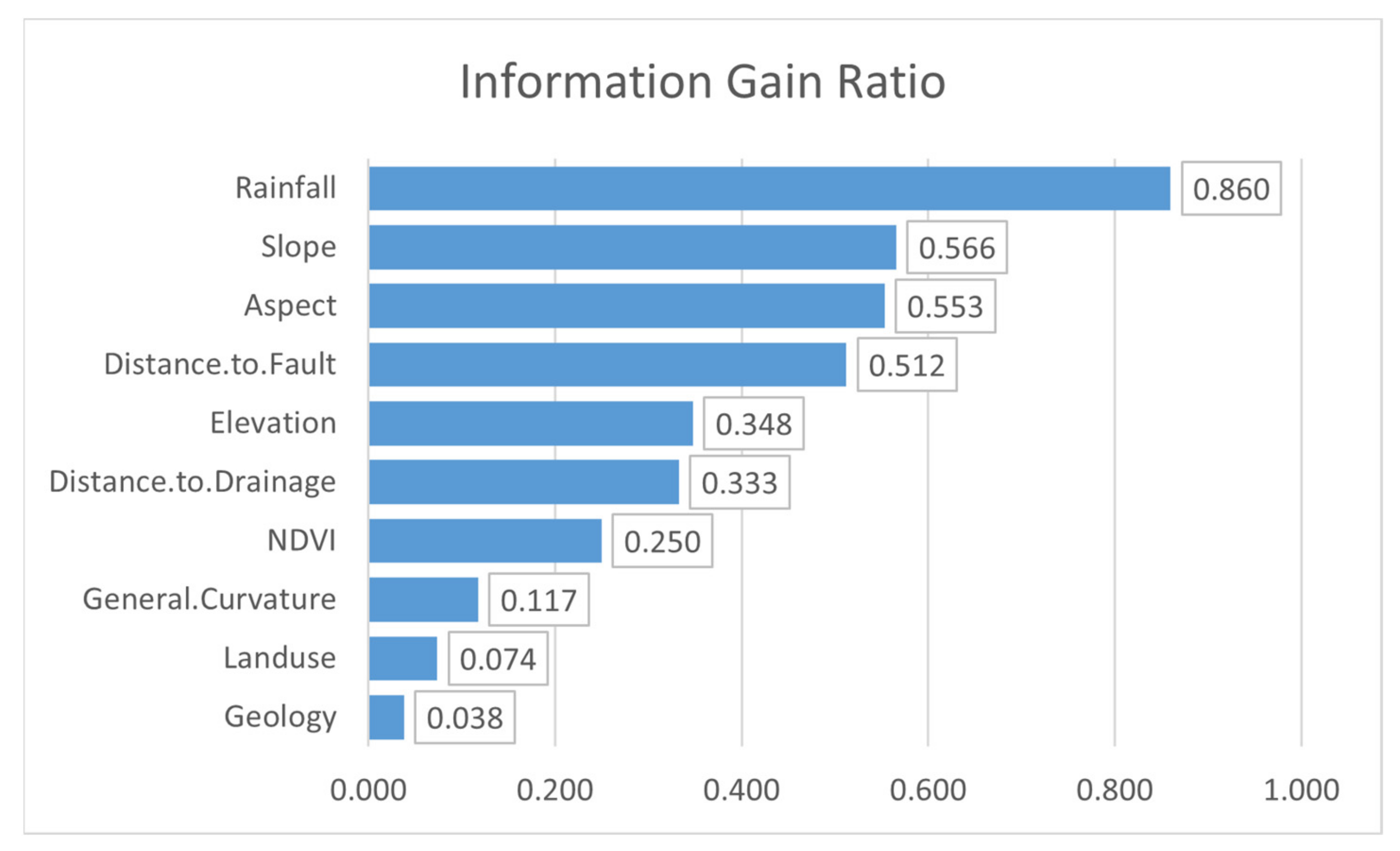
In landslide susceptibility studies, it is advised that researchers study the importance and mechanisms of each influencing factor because this can guide the prediction and prevention of landslide disasters [82]. The information gain ratio results (Figure 6) show that all the ten conditioning factors can be used for modeling landslide susceptibility in Awgu. In addition, the conditioning factors were sorted and ranked in the order of their contribution by listing the scores of the IGR from the highest value to the lowest value, such as rainfall (0.860), slope (0.566), aspect (0.553), distance to fault (0.512), elevation (0.348), distance to drainage (0.333), NDVI (0.250), general curvature (0.117), land use (0.074), and geology (0.038). Afterwards, all ten conditioning factors were further used for the landslide susceptibility analysis.
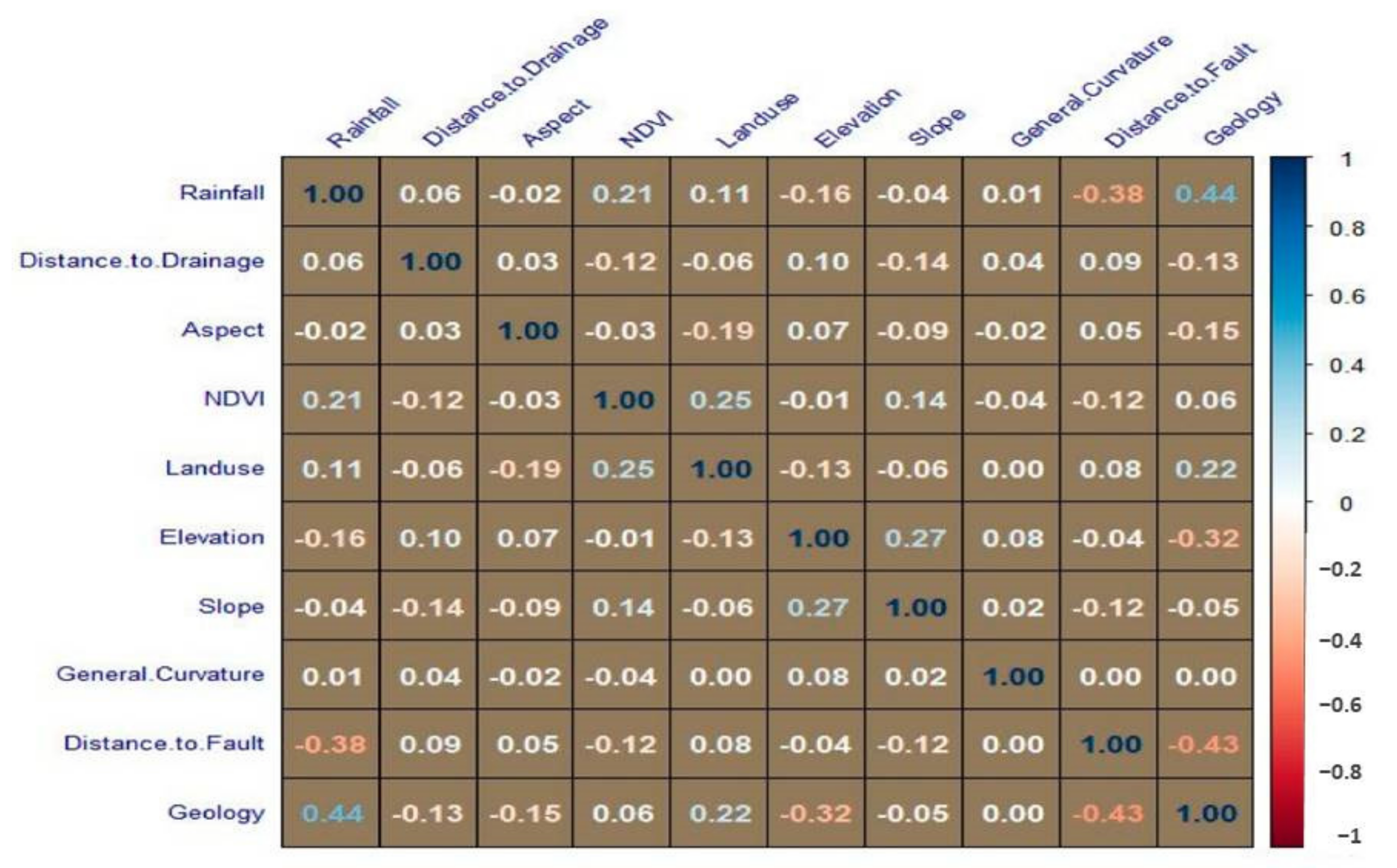
In addition, multicollinearity among the ten conditioning factors was also identified using the Pearson correlation coefficient (Figure 7). A correlation coefficient greater than 0 signifies a positive correlation and moves in the same direction. The results show that NDVI, land use, slope, and elevation have a good relationship. Additionally, the highest number of correlation coefficients was observed between rainfall (0.44) and geology (0.44) (Figure 7).

4.2. Generation of Landslide Susceptibility Maps of the Study Area

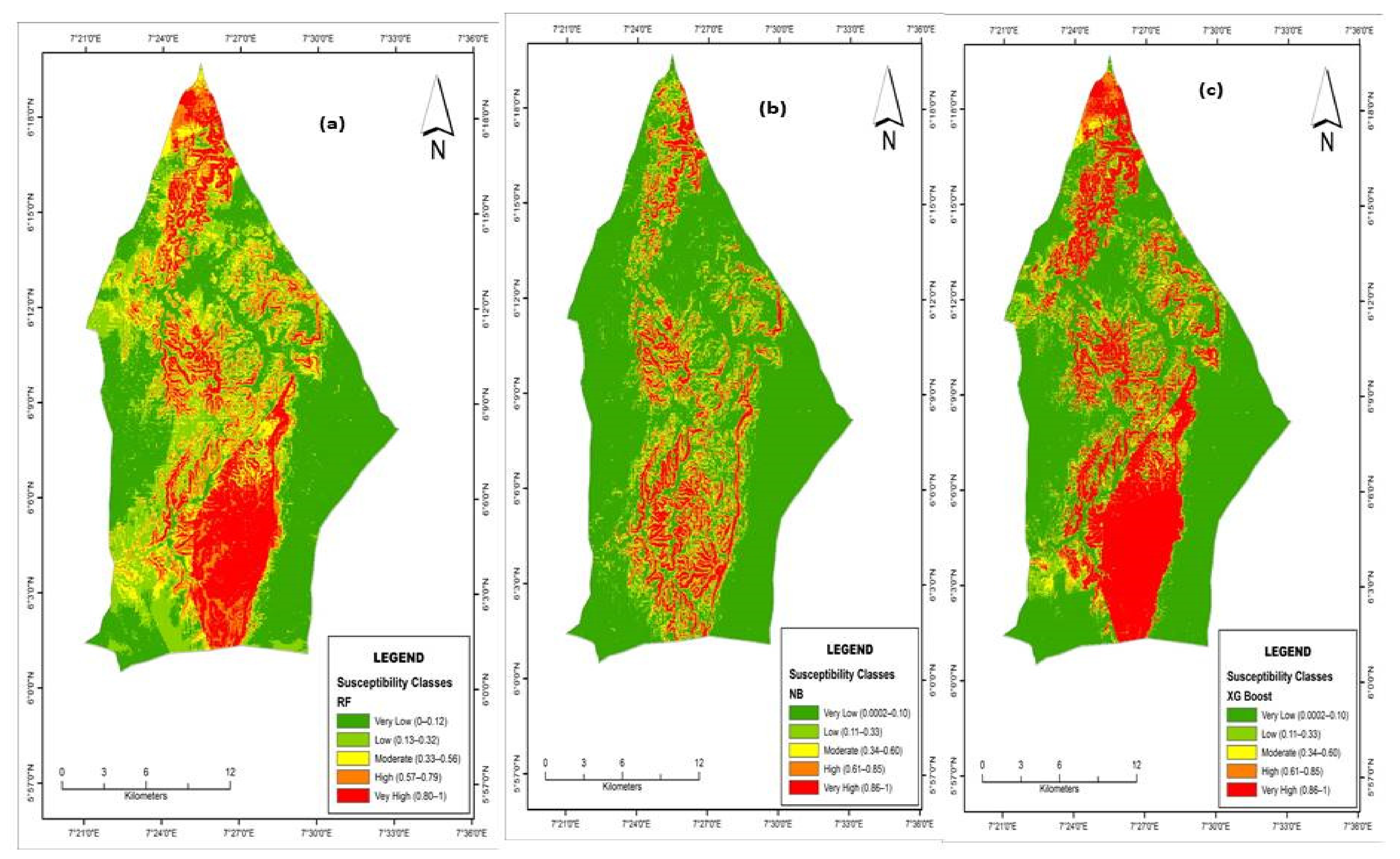
As determined by previous researcher [83], landslide susceptibility maps are generated using an assessment of the spatial distribution of the landslide probability in a given area based on local geo-environmental factors. The landslide susceptibility models used the training datasets and the validation sets. The landslide susceptibility index was calculated from 0 to 1 using RF, Xgboost, and NB models. From previous expert experiences, classification methods should be used to divide the histogram of the landslide susceptibility map into different parts for a better extraction of the susceptible zones [84]. Therefore, to achieve a classification in the study area, the landslide susceptibility index was classified using the natural break technique, which discriminated five susceptibility classes (very high, high, moderate, low, and not susceptible classes).
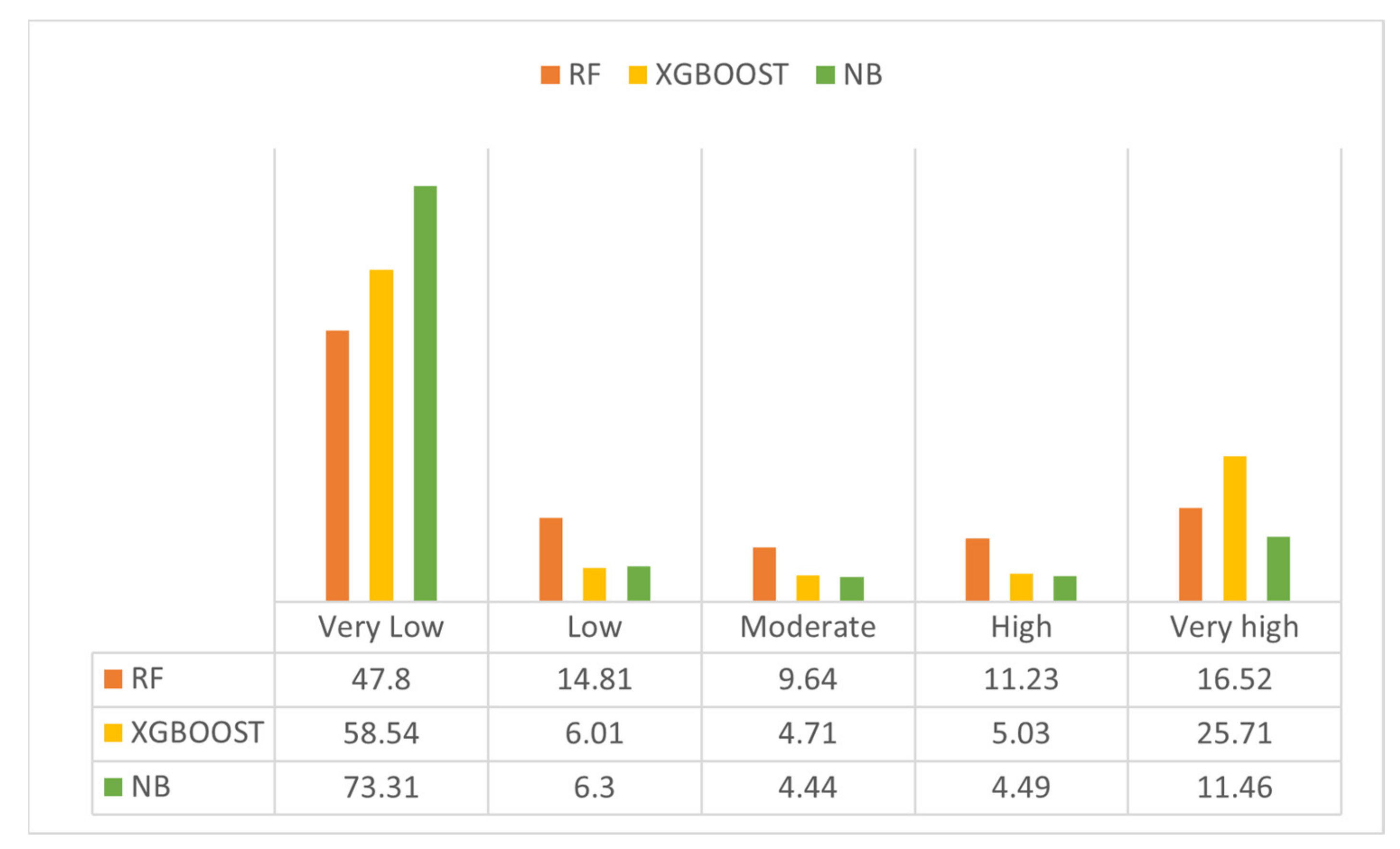
The area coverage of the landslide susceptibility is highly concentrated in the northern, middle, and southern parts of Awgu (Figure 8a–c). The percentage distribution (Figure 9) of each susceptibility class in the RF model revealed that 47.80% of the study area falls into the not susceptible class, 14.81 % accounts for the low susceptibility class, and 9.64% falls into the moderately susceptible class. Whereas 11.23% of the study area falls into the highly susceptible class, and the very highly susceptible class accounts for 16.52%. The NB model shows that 73.31% of the study area falls into the not susceptible class, 6.30% into the low susceptibility class, 4.44% into the moderately susceptible class, 4.49% into the highly susceptible class, and 11.46% into the very highly susceptible class. The XGBOOST model shows that 58.54% of the study area falls into the not susceptible class, the low class accounts for 6.01%, 4.71% falls into the moderately susceptible class, 5.03% falls into the highly susceptible class, and 25.71% accounts for the very highly susceptible class.

4.3. Accuracy and Comparisons of the Models

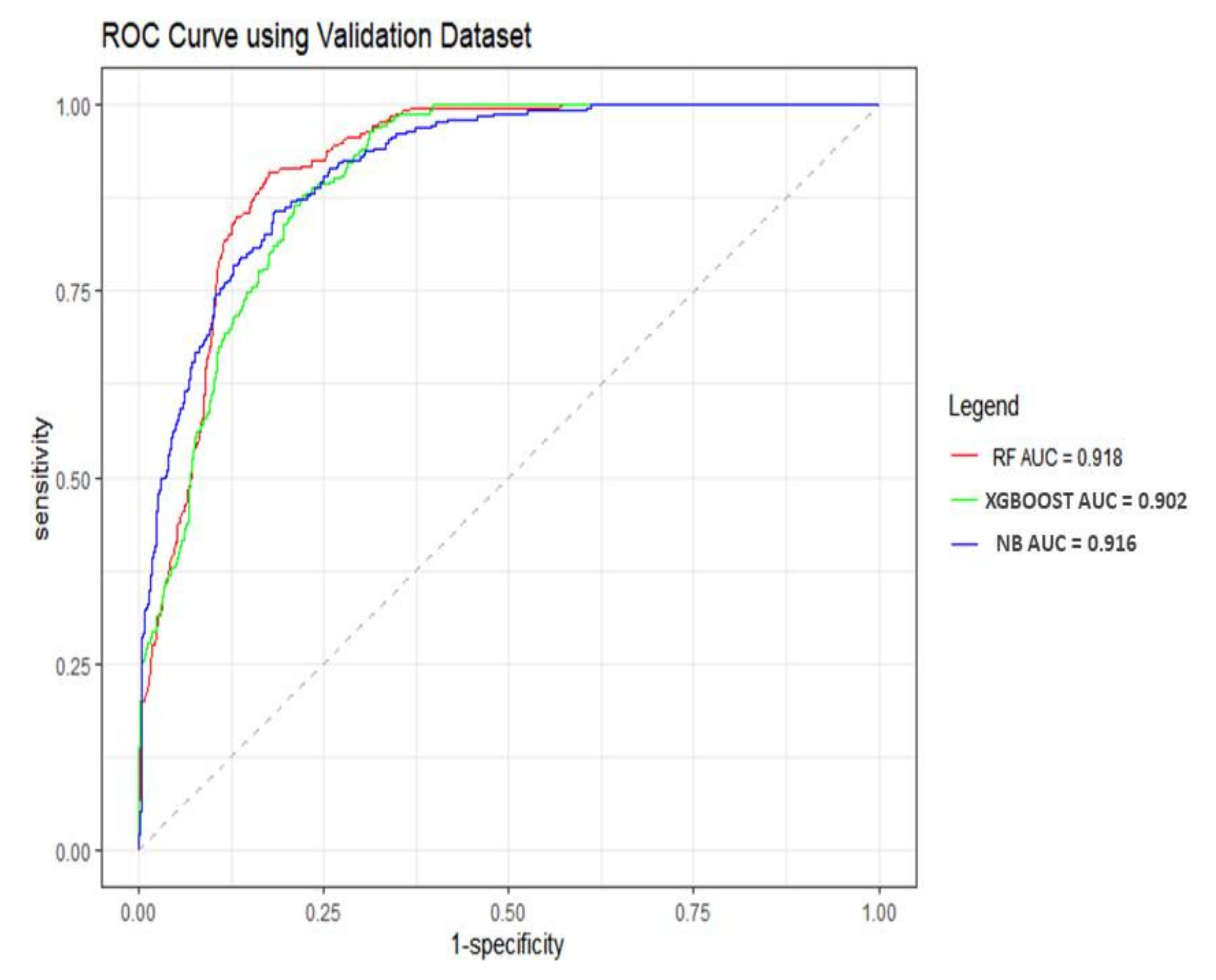
In this study, the performance produced by the three models of RF, XGBOOST, and NB algorithms based on the testing dataset is summarized in Table 1. Although all the models show excellent performance with respect to the landslide susceptibility assessment in the study area, the landslide susceptibility map produced with the RF algorithm had the best predictive performance with an AUC of 0.918, followed by the NB model (AUC 0.916), and the lowest predictive performance was the XGBOOST algorithm (AUC 0.902). the RF algorithm shows the best recognition ability with respect to landslide pixels in the Kappa index, specificity, and PPV. Then, the NB algorithm seems to outperform the rest of the models in terms of ACC, specificity, and NPV.

5. Discussion

5.1. Brief Outlines of Mapped Slides (Inventory)

According to experts, the higher the warning zone for landslide hazards, the greater the probability of a landslide [85]. Therefore, landslide inventory generation is a crucial stage [86]. Through a scientific analysis of landslides, we can assess and locate risky landslide-prone areas [87]. In the current study, the easy extraction of binary attributes set to 1 and 0 (presence and absence of landslide) was performed with 56 polygonal representations of past landslides, a laGriSu tool pack [44], and a digital elevation model. The following steps were taken to extract landslide and non–landslide samples. Step 1: The grid unit extraction of slope values for the original inventory. Here, we extracted the distribution of landslides on the slope and identified the threshold of the slope that did not witness any landslide (as a safe area). Step 2: We extracted the landslide-free inventory based on two assumptions—firstly, we assigned a buffer distance of 250 m from each landslide location considered to be a safe area, and secondly, we integrated the threshold of the slope of the study area of 8 degrees and also the buffer given to us by the slope-limited and buffer distance-limited landslides, and 56 polygons of a landslide-free inventory were also extracted. Step 3: we extracted the training and testing landslide samples using 70% for the training percentage (training 1 and 0) and 30% of the grid unit width in meters (DEM) for testing (1 and 0) by integrating the parameters of the 56 polygons of the landslide-free inventory, the landslide within the slope value, and the slope raster, and determined the training and testing zones. Step 4: we attached 10 conditioning factors to the training and testing datasets and extracted all the values for modeling landslide susceptibility

5.2. The Role of the Conditioning Factors

Over the years, the details on landslide susceptibility have proven to be a combination of direct and effective methods in delineating the relationship between landslides and conditioning factors. Landslide inventories analyzed with the conditioning factors can provide useful information for spatial models [86]. These parameters significantly affect landslide disaster prediction and prevention [56]. However, there is no definite table for landslides’ conditioning factors. Experts caution that selecting unbiased and appropriate factors for mapping landslide susceptibility should be a primary consideration [26]. According to Chen et al. [59], determining the importance of conditioning factors in landslide susceptibility mapping is also important in landslide studies. In line with this, the information gain ratio results suggest that rainfall acts as the most important conditioning factor, and most landslide occurrences happen during the rainy season [3]. Rainfall can continuously undermine the slope, enhance the slope erosion, increase runoff, increase the pore water pressure of rock and soil masses, and will eventually lead to landslides. Other important morphometric factors contributing to landslide occurrence in the study region include the slope, aspect, and distance to the fault. The relationship between the slope and a landslide may be attributed to the saturation, and a high pore water pressure can initiate the slip plane. The aspect also greatly impacts landslides in the area because of the correlation between rainfall and aspects. The aspects, as categorical data, were converted into eight numeric classes of 45 degrees (a–h) and used for the landslide analysis.
Furthermore, the distance to fault also shows a great effect on landslides because where the faults exist, rock fissures will develop, rainwater infiltration will become easier, and landslides in the region will occur with numerous identifiable lineaments that can be observed along the faults. Although a lower IGR value was observed with respect to land use and geology to ascertain the distribution of landslide susceptibility in the area, in this paper, land use and geology were also used as categorical data, and all the conditioning factors were used to produce landslide susceptibility modeling because they were above 0.01 and showed no redundancy. In addition, assessing the correlation of the selected conditioning factors with past and present events can provide appropriate factors to improve the performance of landslide susceptibility models [88]; the results of the Pearson correlation coefficient showed that there seem to be both positive and negative correlations between the conditioning factors. Variables such as rainfall and geology (Figure 7) have the highest correlation coefficients. However, they are less than the critical value of 0.7, implying that there is no high correlation between the conditioning factors [50].

5.3. Performance of the Models in Susceptibility

This paper employed three machine learning models (RF, XGBOOST, and NB) in Awgu/Nigeria. The entire study area was used to produce LSM (Figure 8) and percentage of each susceptibility class of the models was determined (Figure 9). The models’ performance metrics show a high prediction accuracy that was better than the previous study [89], indicating their suitability for landslide susceptibility mapping in the area. The RF model is marginally the most stable model as it performed the best since the number of trees chosen to create the models is fundamental to the stability of the models and ensures high accuracy and generalization for measuring the relationship between external factors and landslide movements [90,91]. In some landslide studies, RF models have proven to be a promising technique and outperform other models [92,93]. The NB model shows limitations in learning the interactions between the conditioning factors and performs best without multicollinearity [33]. However, it can be considered a reliable tool for landslide susceptibility mapping when initializing low-complexity models and small datasets [33]. The XGBOOST model, as shown in the AUC (Figure 10), has the lowest predictive performance in the study area.
Identifying and mapping landslide-prone areas is necessary to curb future landslide events and to achieve accurate and sustainable control operations to prevent future landslide events. The machine learning algorithms employed for the landslide susceptibility assessment in this study show excellent results and have advantages in landslide monitoring, modeling, and prediction, and show stability with multiple datasets, which can be helpful to decision makers regarding landslide mitigation and control management.

6. Conclusions

Machine learning can be reliable with respect to reducing the uncertainty and accuracy for appropriately mapping of regional landslide susceptibility. In this paper, an adequate geospatial database of Awgu, southeastern Nigeria, was generated in combination with past landslides, and 10 conditioning factors with different machine learning models were used for the landslide susceptibility map, which is key for controlling and preventing landslide disasters. Rainfall showed a greater significance regarding the occurrence of landslides in the study area, and land use was the least significant with respect to landslide occurrences. The outcome of the experiment revealed that Awgu is prone to landslides. The landslides are concentrated in the region’s north, middle, and southern parts, which fall into high and very-high landslide susceptibility areas.
Furthermore, the performance of the different models shows excellent accuracy, with the RF model being the best predictive model in the study, followed by the NB models, and the least predictive model is that of XGBOOST. Conclusively, this work can be used for various decision support systems for landslide mitigation and management control in Nigeria and as a reference in areas with similar conditions.

Author Contributions

Conceptualization, S.Q. (Shengwu Qin) and U.E.N.; methodology, U.E.N., software, U.E.N., validation, U.E.N., J.Y. and S.J.; formal analysis, U.E.N., data curation, S.Q. (Shengwu Qin), U.E.N., J.Y. and (N.C.C.); writing—original draft preparation, U.E.N., O.A.A. and E.M.E.; writing-review and editing, U.E.N., O.A.A., S.Q. (Shuangshuang Qiao) and S.J.; Visualization, U.E.N., N.C.C., S.Q. (Shuangshuang Qiao), S.J. and E.M.E.; supervision, S.Q. (Shengwu Qin); project administration, S.Q. (Shengwu Qin); funding acquisition, S.Q. (Shengwu Qin). All authors have read and agreed to the published version of the manuscript.

Funding

This work was supported by the National Natural Science Foundation of China (Grant No. 47041977221 and 41972267) and by the Jilin Provincial Science and Technology Department 471 (No. 20190303103SF).

Institutional Review Board Statement

Not applicable.

Informed Consent Statement

Not applicable.

Data Availability Statement

Not applicable.

Conflicts of Interest

The authors declare no conflict of interest.

References

  1. Igwe, O. The study of the factors controlling rainfall-induced landslides at a failure-prone catchment area in Enugu, Southeastern Nigeria using remote sensing data. Landslides 2015, 12, 1023–1033. [Google Scholar] [CrossRef]
  2. Arabameri, A.; Reza, H.; Mojtaba, P. Applying different scenarios for landslide spatial modeling using computational intelligence methods. Environ. Earth Sci. 2017, 76, 832. [Google Scholar] [CrossRef]
  3. Igwe, O. Predisposing factors and the mechanisms of rainfall-induced slope movements in Ugwueme, South-East Nigeria. Bull. Eng. Geol. Environ. 2016, 75, 623–636. [Google Scholar] [CrossRef]
  4. Tian, G.; Jiang, J.; Yang, Z.; Zhang, Y. The urban growth, size distribution and spatio-temporal dynamic pattern of the Yangtze River Delta megalopolitan region, China. Ecol. Modell. 2011, 222, 865–878. [Google Scholar] [CrossRef]
  5. Yang, X.; Damen, M.C.J.; Van Zuidam, R.A. Satellite remote sensing and GIS for the analysis of channel migration changes in the active Yellow River Delta, China. Int. J. Appl. Earth Obs. Geoinf. 1999, 1, 146–157. [Google Scholar] [CrossRef]
  6. He, Q.; Shahabi, H.; Shirzadi, A.; Li, S.; Chen, W.; Wang, N.; Chai, H.; Bian, H.; Ma, J.; Chen, Y.; et al. Landslide spatial modelling using novel bivariate statistical based Naïve Bayes, RBF Classifier, and RBF Network machine learning algorithms. Sci. Total Environ. 2019, 663, 1–15. [Google Scholar] [CrossRef]
  7. Alireza, A.; Biswajeet, P.; Khalil, R.; Saro, L.; Masoud, S. An ensemble model for landslide susceptibility mapping in a forested area. Geocarto Int. 2020, 35, 1680–1705. [Google Scholar] [CrossRef]
  8. Arabameri, A.; Saha, S.; Roy, J.; Chen, W.; Blaschke, T.; Bui, D.T. Landslide Susceptibility Evaluation and Management Using Different Machine Learning Methods in the Gallicash River Watershed, Iran. Remote Sens. 2020, 12, 475. [Google Scholar] [CrossRef]
  9. Pradhan, B. GIS-based landslide susceptibility mapping using numerical risk factor bivariate model and its ensemble with linear multivariate algorithms and boosted regression tree. J. Mt. Sci. 2019, 16, 595–618. [Google Scholar]
  10. Pellicani, R.; Van Westen, C.J.; Spilotro, G. Assessing landslide exposure in areas with limited landslide information. Landslides 2014, 11, 463–480. [Google Scholar] [CrossRef]
  11. Van Westen, C.J.; Rengers, N.; Soeters, R. Use of geomorphological information in indirect landslide susceptibility assessment. Nat. Hazards 2003, 30, 399–419. [Google Scholar] [CrossRef]
  12. Aleotti, P.; Chowdhury, R. Landslide hazard assessment: Summary review and new perspectives. Bull. Eng. Geol. Environ. 1999, 58, 21–44. [Google Scholar] [CrossRef]
  13. Chakraborty, T.; Alam, M.S.; Islam, M.D. Landslide Susceptibility Mapping Using Xgboost Model in Chittagong District, Bangladesh. In Proceedings of the International Conference on Disaster Risk Management, Dhaka, Bangladesh, 12–14 January 2019. [Google Scholar]
  14. Biodiversit, S.F.; Prof, S.; Teimouri, M.; Graee, P.; Geological, J.; Of, S.; Lee, S.; Bureau, G.; Resources, N.; Avenue, N. Landslide Classification, Characterization and Susceptibility Modeling in Kwazulu-Nata. Ph.D. Thesis, University of the Witwatersrand, Johannesburg, South Africa.
  15. Ma, Z.; Qin, S.; Cao, C.; Lv, J.; Li, G.; Qiao, S.; Hu, X. The influence of different knowledge-driven methods on landslide susceptibility mapping: A case study in the Changbai Mountain Area, Northeast China. Entropy 2019, 21, 372. [Google Scholar] [CrossRef]
  16. Chen, T.; Niu, R.; Du, B.; Wang, Y. Landslide spatial susceptibility mapping by using GIS and remote sensing techniques: A case study in Zigui County, the Three Georges reservoir, China. Environ. Earth Sci. 2015, 73, 5571–5583. [Google Scholar] [CrossRef]
  17. Huang, F.; Cao, Z.; Guo, J.; Jiang, S.H.; Li, S.; Guo, Z. Comparisons of heuristic, general statistical and machine learning models for landslide susceptibility prediction and mapping. Catena 2020, 191, 104580. [Google Scholar] [CrossRef]
  18. Nsengiyumva, J.B.; Valentino, R. Predicting landslide susceptibility and risks using GIS-based machine learning simulations, case of upper Nyabarongo catchment. Geomat. Nat. Hazards Risk 2020, 11, 1250–1277. [Google Scholar] [CrossRef]
  19. Shirzadi, A.; Soliamani, K.; Habibnejhad, M.; Kavian, A.; Chapi, K.; Shahabi, H.; Chen, W.; Khosravi, K.; Thai Pham, B.; Pradhan, B.; et al. Novel GIS based machine learning algorithms for shallow landslide susceptibility mapping. Sensors 2018, 18, 3777. [Google Scholar] [CrossRef]
  20. Youssef, A.M.; Pourghasemi, H.R. Landslide susceptibility mapping using machine learning algorithms and comparison of their performance at Abha Basin, Asir Region, Saudi Arabia. Geosci. Front. 2021, 12, 639–655. [Google Scholar] [CrossRef]
  21. Kim, J.C.; Lee, S.; Jung, H.S.; Lee, S. Landslide susceptibility mapping using random forest and boosted tree models in Pyeong-Chang, Korea. Geocarto. Int. 2018, 33, 1000–1015. [Google Scholar] [CrossRef]
  22. Bui, D.T.; Shahabi, H.; Shirzadi, A.; Chapi, K.; Alizadeh, M.; Chen, W.; Mohammadi, A.; Ahmad, B.B.; Panahi, M.; Hong, H.; et al. Landslide detection and susceptibility mapping by AIRSAR data using support vector machine and index of entropy models in Cameron Highlands, Malaysia. Remote Sens. 2018, 10, 1527. [Google Scholar]
  23. Gorsevski, P.V.; Brown, M.K.; Panter, K.; Onasch, C.M.; Simic, A.; Snyder, J. Landslide detection and susceptibility mapping using LiDAR and an artificial neural network approach: A case study in the Cuyahoga Valley National Park, Ohio. Landslides 2016, 13, 467–484. [Google Scholar] [CrossRef]
  24. Zare, M.; Pourghasemi, H.R.; Vafakhah, M.; Pradhan, B. Landslide susceptibility mapping at Vaz Watershed (Iran) using an artificial neural network model: A comparison between multilayer perceptron (MLP) and radial basic function (RBF) algorithms. Arab J. Geosci. 2013, 6, 2873–2888. [Google Scholar] [CrossRef]
  25. Pham, B.T.; Vu, V.D.; Costache, R.; Van Phong, T.; Ngo, T.Q.; Tran, T.-H.; Nguyen, H.D.; Amiri, M.; Tan, M.T.; Trinh, P.T.; et al. Landslide susceptibility mapping using state-of-the-art machine learning ensembles. Geocarto. Int. 2021, 37, 5175–5200. [Google Scholar] [CrossRef]
  26. Arabameri, A.; Pal, S.C.; Rezaie, F.; Saha, A.; Blaschke, T.; Di Napoli, M.; Ghorbanzadeh, O.; Ngo, P.T.T. Decision tree based ensemble machine learning approaches for landslide susceptibility mapping. Geocarto. Int. 2021, 37, 1–35. [Google Scholar] [CrossRef]
  27. Zhang, F.; Zhu, Y.; Zhao, X.; Zhang, Y.; Shi, L.; Liu, X. Spatial Distribution and Identification of Hidden Danger Points of Landslides Based on Geographical Factors. Wuhan Daxue Xuebao Geomat. Inf. Sci. Wuhan Univ. 2020, 45, 1233–1244. [Google Scholar] [CrossRef]
  28. Cao, J.; Zhang, Z.; Du, J.; Zhang, L.; Song, Y.; Sun, G. Multi-geohazards susceptibility mapping based on machine learning—A case study in Jiuzhaigou, China. Nat. Hazards 2020, 102, 851–871. [Google Scholar] [CrossRef]
  29. Chen, W.; Panahi, M.; Pourghasemi, H.R. Performance evaluation of GIS-based new ensemble data mining techniques of adaptive neuro-fuzzy inference system (ANFIS) with genetic algorithm (GA), differential evolution (DE), and particle swarm optimization (PSO) for landslide spatial modelling. Catena 2017, 157, 310–324. [Google Scholar] [CrossRef]
  30. Pradhan, B. A comparative study on the predictive ability of the decision tree, support vector machine and neuro-fuzzy models in landslide susceptibility mapping using GIS. Comput. Geosci. 2013, 51, 350–365. [Google Scholar] [CrossRef]
  31. Hong, H.; Miao, Y.; Liu, J.; Zhu, A.X. Exploring the effects of the design and quantity of absence data on the performance of random forest-based landslide susceptibility mapping. Catena 2019, 176, 45–64. [Google Scholar] [CrossRef]
  32. Zhang, K.; Wu, X.; Niu, R.; Yang, K.; Zhao, L. The assessment of landslide susceptibility mapping using random forest and decision tree methods in the Three Gorges Reservoir area, China. Environ. Earth Sci. 2017, 76, 405. [Google Scholar] [CrossRef]
  33. Tsangaratos, P.; Ilia, I. Comparison of a logistic regression and Naïve Bayes classifier in landslide susceptibility assessments: The influence of models complexity and training dataset size. Catena 2016, 145, 164–179. [Google Scholar] [CrossRef]
  34. Pham, B.T.; Bui, D.T.; Dholakia, M.B.; Prakash, I.; Pham, H.V.; Mehmood, K.; Le, H.Q. A novel ensemble classifier of rotation forest and Naïve Bayer for landslide susceptibility assessment at the Luc Yen district, Yen Bai Province (Viet Nam) using GIS. Geomat. Nat. Hazards Risk 2017, 8, 649–671. [Google Scholar] [CrossRef] [Green Version]
  35. Arabameri, A.; Santosh, M.; Saha, S.; Ghorbanzadeh, O.; Roy, J.; Tiefenbacher, J.P.; Moayedi, H.; Costache, R. Spatial prediction of shallow landslide: Application of novel rotational forest-based reduced error pruning tree. Geomat. Nat. Hazards Risk 2021, 12, 1343–1370. [Google Scholar] [CrossRef]
  36. Sahin, E.K. Assessing the predictive capability of ensemble tree methods for landslide susceptibility mapping using XGBoost, gradient boosting machine, and random forest. SN Appl. Sci. 2020, 2, 1308. Available online: http://link.springer.com/10.1007/s42452-020-3060-1 (accessed on 7 October 2021). [CrossRef]
  37. Pradhan, A.M.S.; Kim, Y.T. Rainfall-induced shallow landslide susceptibility mapping at two adjacent catchments using advanced machine learning algorithms. ISPRS Int. J. Geo.-Inf. 2020, 9, 569. [Google Scholar] [CrossRef]
  38. Belgiu, M.; Drăgu, L. Random forest in remote sensing: A review of applications and future directions. ISPRS J. Photogramm. Remote Sens. 2016, 114, 24–31. [Google Scholar] [CrossRef]
  39. Georganos, S.; Grippa, T.; Vanhuysse, S.; Lennert, M.; Shimoni, M.; Wolff, E. Very High Resolution Object-Based Land Use-Land Cover Urban Classification Using Extreme Gradient Boosting. IEEE Geosci. Remote Sens. Lett. 2018, 15, 607–611. [Google Scholar] [CrossRef]
  40. Soria, D.; Garibaldi, J.M.; Ambrogi, F.; Biganzoli, E.M.; Ellis, I.O. Knowledge-Based Systems A ‘non-parametric’ version of the naive Bayes classifier. Knowl.-Based Syst. 2011, 24, 775–784. [Google Scholar] [CrossRef]
  41. Dou, J.; Paudel, U.; Oguchi, T.; Uchiyama, S.; Hayakawa, Y.S. Shallow and deep-seated landslide differentiation using support vector machines: A case study of the chuetsu area, Japan. Terr. Atmos. Ocean. Sci. 2015, 29, 227–239. [Google Scholar] [CrossRef]
  42. Tien Bui, D.; Pradhan, B.; Lofman, O.; Revhaug, I. Landslide susceptibility assessment in vietnam using support vector machines, decision tree, and nave bayes models. Math. Probl. Eng. 2012, 2012, 974638. [Google Scholar] [CrossRef]
  43. Huang, F.; Zhang, J.; Zhou, C.; Wang, Y.; Huang, J.; Zhu, L. A deep learning algorithm using a fully connected sparse autoencoder neural network for landslide susceptibility prediction. Landslides 2020, 17, 217–229. [Google Scholar] [CrossRef]
  44. Althuwaynee, O.F.; Aydda, A.; Hwang, I.; Kim, S.W. LAGRISU Toolpack for the Automatic Extraction of Grid Units and Slope Units Applications to Inje Province South Korea. Available online: https://www.researchgate.net/publication/348249510 (accessed on 28 February 2022).
  45. Yao, J.; Qin, S.; Qiao, S.; Liu, X.; Zhang, L.; Chen, J. Application of a two-step sampling strategy based on deep neural network for landslide susceptibility mapping. Bull. Eng. Geol. Environ. 2022, 81, 4. [Google Scholar] [CrossRef]
  46. Huang, F.; Yao, C.; Liu, W.; Li, Y.; Liu, X. Landslide susceptibility assessment in the Nantian area of China: A comparison of frequency ratio model and support vector machine. Geomat. Nat. Hazards Risk 2018, 9, 919–938. [Google Scholar] [CrossRef]
  47. Luo, X.; Lin, F.; Zhu, S.; Yu, M.; Zhang, Z.; Meng, L.; Peng, J. Mine landslide susceptibility assessment using IVM, ANN and SVM models considering the contribution of affecting factors. PLoS ONE 2019, 14, e0215134. [Google Scholar] [CrossRef]
  48. Bui, D.T.; Tuan, T.A. Spatial prediction models for shallow landslide hazards: A comparative assessment of the efficacy of support vector machines, artificial neural networks, kernel logistic regression, and logistic model tree. Landslides 2015, 13, 361–378. [Google Scholar]
  49. Yao, J.; Qin, S.; Qiao, S.; Che, W.; Chen, Y.; Su, G.; Miao, Q. Assessment of landslide susceptibility combining deep learning with semi-supervised learning in Jiaohe County, Jilin Province, China. Appl. Sci. 2020, 10, 5640. [Google Scholar] [CrossRef]
  50. Hong, H.; Liu, J.; Zhu, A.X. Modeling landslide susceptibility using LogitBoost alternating decision trees and forest by penalizing attributes with the bagging ensemble. Sci. Total Environ. 2020, 718, 137231. [Google Scholar] [CrossRef]
  51. Moore, I.D.; Grayson, R.B.; Ladson, A.R. Digital terrain modelling: A review of hydrological, geomorphological, and biological applications. Hydrol. Process. 1991, 5, 3–30. [Google Scholar] [CrossRef]
  52. Qi, S.; Xu, Q.; Lan, H.; Zhang, B.; Liu, J. Spatial distribution analysis of landslides triggered by 2008.5.12 Wenchuan Earthquake, China. Eng. Geol. 2010, 116, 95–108. [Google Scholar] [CrossRef]
  53. Baeza, C.; Corominas, J. Assessment of shallow landslide susceptibility by means of multivariate statistical techniques. Earth Surf. Process. Landf. 2001, 26, 1251–1263. [Google Scholar] [CrossRef]
  54. Aksoy, B.; Ercanoglu, M. Landslide identification and classification by object-based image analysis and fuzzy logic: An example from the Azdavay region (Kastamonu, Turkey). Comput. Geosci. 2012, 38, 87–98. [Google Scholar] [CrossRef]
  55. Gökceoglu, C.; Aksoy, H. Landslide susceptibility mapping of the slopes in the residual soils of the Mengen region (Turkey) by deterministic stability analyses and image processing techniques. Eng. Geol. 1996, 44, 147–161. [Google Scholar] [CrossRef]
  56. Wang, Y.; Wen, H.; Sun, D.; Li, Y. Quantitative assessment of landslide risk based on susceptibility mapping using random forest and geodetector. Remote Sens. 2021, 13, 2625. [Google Scholar] [CrossRef]
  57. Hashim, H.; Abd Latif, Z.; Adnan, N.A. Urban Vegetation Classification with Ndvi Threshold Value Method with Very High Resolution (Vhr) Pleiades Imagery. Int. Arch. Photogramm. Remote Sens. Spat. Inf. Sci.-ISPRS Arch. 2019, 42, 237–240. [Google Scholar] [CrossRef]
  58. Kayastha, P.; Dhital, M.R.; De Smedt, F. Application of the analytical hierarchy process (AHP) for landslide susceptibility mapping: A case study from the Tinau watershed, west Nepal. Comput. Geosci. 2013, 52, 398–408. [Google Scholar] [CrossRef]
  59. Chen, W.; Pourghasemi, H.R.; Naghibi, S.A. Prioritization of landslide conditioning factors and its spatial modeling in Shangnan County, China using GIS-based data mining algorithms. Bull. Eng. Geol. Environ. 2018, 77, 611–629. [Google Scholar] [CrossRef]
  60. Segoni, S.; Pappafico, G.; Luti, T.; Catani, F. Landslide susceptibility assessment in complex geolog-ical settings: Sensitivity to geological information and insights on its parameterization. Landslides 2020, 2019, 2443–2453. [Google Scholar] [CrossRef]
  61. Huang, F.; Yin, K.; Huang, J.; Gui, L.; Wang, P. Landslide susceptibility mapping based on self-organizing-map network and extreme learning machine. Eng. Geol. 2017, 223, 11–22. [Google Scholar] [CrossRef]
  62. Pradhan, B.; Lee, S.; Buchroithner, M.F. A GIS-based back-propagation neural network model and its cross-application and validation for landslide susceptibility analyses. Comput. Environ. Urban Syst. 2010, 34, 216–235. [Google Scholar] [CrossRef]
  63. Rabby, Y.W.; Hossain, M.B.; Abedin, J. Landslide susceptibility mapping in three Upazilas of Rangamati hill district Bangladesh: Application and comparison of GIS-based machine learning methods. Geocarto. Int. 2020, 37, 3371–3396. [Google Scholar] [CrossRef]
  64. Chen, T.; Guestrin, C. XG Boost:A scalable tree boosting system. In Proceedings of the 22nd ACM SIGKDD International Conference on Knowledge Discovery and Data Mining-KDD, San Francisco, CA, USA, 13–17 August 2016; ACM Press: New York, NY, USA, 2016; pp. 785–794. [Google Scholar]
  65. AlThuwaynee, O.F.; Kim, S.W.; Najemaden, M.A.; Aydda, A.; Balogun, A.L.; Fayyadh, M.M.; Park, H.-J. Demystifying uncertainty in PM10 susceptibility mapping using variable drop-off in extreme-gradient boosting (XGB) and random forest (RF) algorithms. Environ. Sci. Pollut. Res. 2021, 28, 43544–43566. [Google Scholar] [CrossRef] [PubMed]
  66. Can, R.; Kocaman, S.; Gokceoglu, C. A comprehensive assessment of XGBoost algorithm for landslide susceptibility mapping in the upper basin of Ataturk dam, Turkey. Appl. Sci. 2021, 11, 4993. [Google Scholar] [CrossRef]
  67. Breiman, L.E.O. Random Forests. Mach. Learn. 2001, 45, 5–32. [Google Scholar] [CrossRef] [Green Version]
  68. Taalab, K.; Cheng, T.; Zhang, Y. Mapping landslide susceptibility and types using Random Forest. Big Earth Data 2018, 2, 159–178. [Google Scholar] [CrossRef]
  69. Miner, A.S.; Vamplew, P.; Windle, D.J.; Flentje, P.; Warner, P. A comparative study of Various Data Mining techniques as applied to the modeling of Landslide susceptibility on the Bellarine Peninsula, Victoria, Australia. In Proceedings of the Geologically Active Proceedings of the 11th IAEG Congress of the International Association of Engineering Geology and the Environment, Auckland, New Zealand, 5–10 September 2010. [Google Scholar]
  70. Dou, J.; Yunus, A.P.; Tien, D.; Merghadi, A.; Sahana, M.; Zhu, Z.; Chen, C.-W.; Khosravi, K.; Yang, Y.; Pham, B.T. Science of the Total Environment Assessment of advanced random forest and decision tree algorithms for modeling rainfall-induced landslide susceptibility in the Izu-Oshima Volcanic Island, Japan. Sci. Total Environ. 2019, 662, 332–346. [Google Scholar] [CrossRef]
  71. Soni, J. Predictive Data Mining for Medical Diagnosis: An Overview of Heart Disease Prediction. Int. J. Comput. Appl. 2011, 17, 43–48. [Google Scholar] [CrossRef]
  72. Lee, S.; Lee, M.; Jung, H.; Lee, S. Landslide susceptibility mapping using Naïve Bayes and Bayesian network models in Umyeonsan, Korea. Geocarto. Int. 2019, 35, 1665–1679. [Google Scholar] [CrossRef]
  73. Thai, B.; Pradhan, B.; Tien, D.; Prakash, I.; Dholakia, M.B. Environmental Modelling & Software A comparative study of different machine learning methods for landslide susceptibility assessment: A case study of Uttarakhand area (India). Environ. Model. Softw. 2016, 84, 240–250. [Google Scholar] [CrossRef]
  74. Sun, D.; Wen, H.; Wang, D.; Xu, J. A random forest model of landslide susceptibility mapping based on hyperparameter optimization using Bayes algorithm. Geomorphology 2020, 362, 107201. [Google Scholar] [CrossRef]
  75. Yu, H.; Chen, G.; Gu, H. A machine learning methodology for multivariate pore-pressure prediction. Comput. Geosci. 2020, 143, 104548. [Google Scholar] [CrossRef]
  76. Stumpf, A.; Kerle, N. Object-oriented mapping of landslides using Random Forests. Remote Sens. Environ. 2011, 115, 2564–2577. [Google Scholar] [CrossRef]
  77. Chen, W.; Shirzadi, A.; Shahabi, H.; Ahmad, B.B.; Zhang, S.; Hong, H.; Zhang, N. A novel hybrid artificial intelligence approach based on the rotation forest ensemble and naïve Bayes tree classifiers for a landslide susceptibility assessment in Langao County, China. Geomat. Nat. Hazards Risk 2017, 8, 1955–1977. [Google Scholar] [CrossRef]
  78. Nhu, V.H.; Mohammadi, A.; Shahabi, H.; Ahmad, B.B.; Al-Ansari, N.; Shirzadi, A.; Clague, J.J.; Jaafari, A.; Chen, W.; Nguyen, H. Landslide susceptibility mapping using machine learning algorithms and remote sensing data in a tropical environment. Int. J. Environ. Res. Public Health 2020, 17, 4933. [Google Scholar] [CrossRef]
  79. Sterlacchini, S.; Ballabio, C.; Blahut, J.; Masetti, M.; Sorichetta, A. Spatial agreement of predicted patterns in landslide susceptibility maps. Geomorphology 2011, 125, 51–61. [Google Scholar] [CrossRef]
  80. Sun, D.; Xu, J.; Wen, H.; Wang, Y. An Optimized Random Forest Model and Its Generalization Ability in Landslide Susceptibility Mapping: Application in Two Areas of Three Gorges Reservoir, China. J. Earth Sci. 2020, 31, 1068–1086. [Google Scholar] [CrossRef]
  81. Goetz, J.N.; Brenning, A.; Petschko, H.; Leopold, P. Evaluating machine learning and statistical prediction techniques for landslide susceptibility modeling. Comput. Geosci. 2015, 81, 1–11. [Google Scholar] [CrossRef]
  82. Wang, S.; Zhuang, J.; Zheng, J.; Fan, H.; Kong, J.; Zhan, J. Application of Bayesian Hyperparameter Optimized Random Forest and XGBoost Model for Landslide Susceptibility Mapping. Front. Earth Sci. 2021, 9, 1–18. [Google Scholar] [CrossRef]
  83. Fell, R.; Corominas, J.; Bonnard, C.; Cascini, L.; Leroi, E.; Savage, W.Z. Guidelines for landslide susceptibility, hazard and risk zoning for land use planning. Eng. Geol. 2008, 102, 85–98. [Google Scholar] [CrossRef]
  84. Althuwaynee, O.F.; Pradhan, B.; Park, H.J.; Lee, J.H. A novel ensemble decision tree-based CHi-squared Automatic Interaction Detection (CHAID) and multivariate logistic regression models in landslide susceptibility mapping. Landslides 2014, 11, 1063–1078. [Google Scholar] [CrossRef]
  85. Huang, F.; Chen, J.; Liu, W.; Huang, J.; Hong, H.; Chen, W. Regional rainfall-induced landslide hazard warning based on landslide susceptibility mapping and a critical rainfall threshold. Geomorphology 2022, 408, 108236. [Google Scholar] [CrossRef]
  86. Ramos-bernal, R.N.; Cant, C.A. Evaluation of Conditioning Factors of Slope Instability and Continuous Change Maps in the Generation of Landslide Inventory Maps Using Machine Learning (ML) Algorithms. Remote Sens. 2021, 13, 4515. [Google Scholar] [CrossRef]
  87. He, S.; Pan, P.; Dai, L.; Wang, H.; Liu, J. Application of kernel-based Fisher discriminant analysis to map landslide susceptibility in the Qinggan River delta, Three Gorges, China. Geomorphology 2012, 171–172, 30–41. [Google Scholar] [CrossRef]
  88. Thai, B.; Nguyen-thoi, T.; Qi, C.; Phong, T.; Van Dou, J. Catena Coupling RBF neural network with ensemble learning techniques for landslide susceptibility mapping. Catena 2020, 195, 104805. [Google Scholar] [CrossRef]
  89. Merghadi, A.; Abderrahmane, B.; Tien Bui, D. Landslide susceptibility assessment at Mila basin (Algeria): A comparative assessment of prediction capability of advanced machine learning methods. ISPRS Int. J. Geo-Inf. 2018, 7, 268. [Google Scholar] [CrossRef]
  90. Segoni, S.; Lagomarsino, D.; Fanti, R.; Moretti, S.; Casagli, N. Integration of rainfall thresholds and susceptibility maps in the Emilia Romagna (Italy) regional-scale landslide warning system. Landslides 2015, 12, 773–785. [Google Scholar] [CrossRef]
  91. Xiao, T.; Yin, K.; Yao, T.; Liu, S. Spatial prediction of landslide susceptibility using GIS-based statistical and machine learning models in Wanzhou County, Three Gorges Reservoir, China. Acta Geochim. 2019, 38, 654–669. [Google Scholar] [CrossRef]
  92. Chen, W.; Peng, J.; Hong, H.; Shahabi, H.; Pradhan, B.; Liu, J.; Zhu, A.-X.; Pei, X.; Duan, Z. Landslide susceptibility modelling using GIS-based machine learning techniques for Chongren County, Jiangxi Province, China. Sci. Total Environ. 2018, 626, 1121–1135. [Google Scholar] [CrossRef]
  93. Chen, W.; Xie, X.; Wang, J.; Pradhan, B.; Hong, H.; Bui, D.T.; Duan, Z.; Ma, J. A comparative study of logistic model tree, random forest, and classification and regression tree models for spatial prediction of landslide susceptibility. Catena 2017, 151, 147–160. [Google Scholar] [CrossRef] [Green Version]
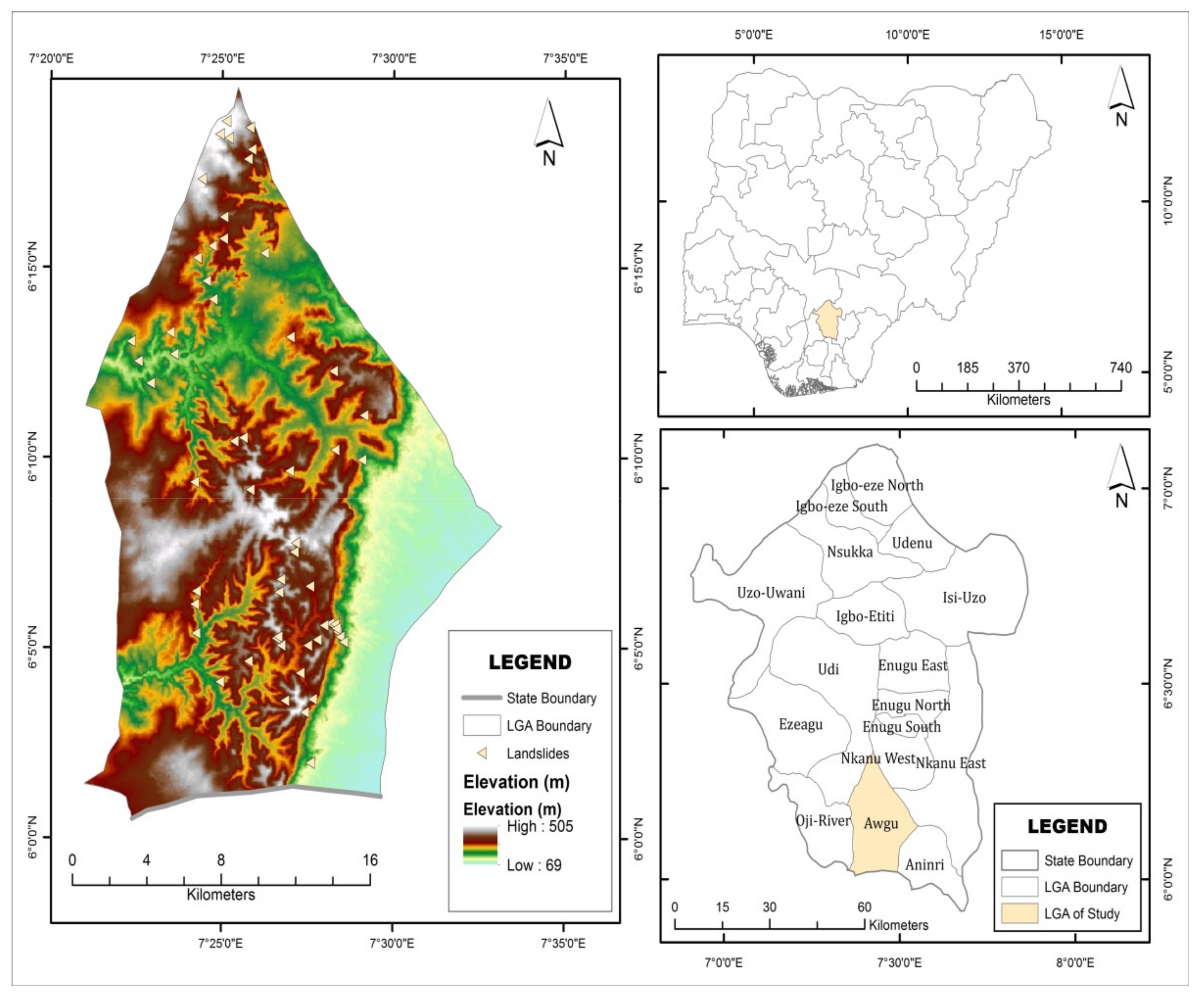
Figure 1. Location of the study area.
Sustainability 14 12000 g001
Figure 2. Flowchart of the study.
Sustainability 14 12000 g002
Figure 3. Pictures of landslides were taken in Awgu (the study area).
Sustainability 14 12000 g003
Figure 4. Landslide conditioning factors used in the study: (a) elevation; (b) slope; (c) aspect; (d) curvature; (e) rainfall; (f) distance to drainage; (g) NDVI; (h) land use; (i) distance to fault; (j) geology.
Sustainability 14 12000 g004aSustainability 14 12000 g004b
Figure 5. Flow chart of RF model.
Sustainability 14 12000 g005
Figure 6. Information gain ratio of the ten conditioning Factors.
Sustainability 14 12000 g006
Figure 7. Pearson correlation coefficient of the ten conditioning factors.
Sustainability 14 12000 g007
Figure 8. Landslide susceptibility map of the study area.
Sustainability 14 12000 g008
Figure 9. Percentage of each susceptibility class of the models.
Sustainability 14 12000 g009
Figure 10. The ROC plot of the various models using the validation set.
Sustainability 14 12000 g010
Table 1. Confusion matrix and statistics of the testing datasets.
ModelConfusion Matrix
TPTNFPFNACCKappaSensitivitySpecificityPPV NPV
RF220784351330.857 0.6300.8550.8630.957 0.623
XGBOOST209741461760.811 0.530 0.808 0.820 0.942 0.543
NB16585390640.869 0.599 0.930 0.6470.905 0.721
Publisher’s Note: MDPI stays neutral with regard to jurisdictional claims in published maps and institutional affiliations.