Article

A Simulation-Based Study of the Influence of Low-Speed Vehicles on Expressway Traffic Safety

1
College of Automobile and Traffic Engineering, Nanjing Forestry University, Nanjing 210037, China
2
College of Civil Engineering, Nanjing Forestry University, Nanjing 210037, China
*
Author to whom correspondence should be addressed.
Sustainability 2022, 14(19), 12165; https://doi.org/10.3390/su141912165
Submission received: 4 September 2022 / Revised: 22 September 2022 / Accepted: 23 September 2022 / Published: 26 September 2022
(This article belongs to the Special Issue Sustainable Transportation Planning and Roadway Safety)

Abstract

:
To reveal the impact mechanism of low-speed vehicles (LSVs) on expressway traffic safety, this paper uses the polynomial fitting method to establish evolution models of traffic density and average speed at different LSV speeds in order to explore the queuing and dissipation characteristics of vehicles affected by LSVs and investigate the impact range of LSVs on expressways. Based on the findings above, this paper builds a Surrogate Safety Assessment Model (SSAM)-based model to quantify driving safety and further explore the differences in vehicle conflicts when an LSV moves in different lanes at the same speed. The simulation experiment is conducted based on the field data from the Inner Ring North Road located along the Nanjing Inner Ring High Speed Road. The results show that the evolutionary features of lane traffic density and average speed under different LSV speeds satisfy the octuple polynomial law, reflecting the spatial heterogeneity of vehicle distribution at different LSV driving speeds. Meanwhile, LSVs with different speeds produced the most significant negative impact on the roadway within 400 m of the expressway entrance. The lower the speed of the LSV, the more significant the adverse effect. In addition, this paper finds that when an LSV travels in different lanes at the same speed, the inner, middle, and outer lanes have the highest number of total conflicts, rear-end conflicts, and lane-change conflicts, respectively. Meanwhile, vehicles in the outer lane are the most significantly affected by LSVs, while vehicles in the middle lane are the least affected with the highest traffic efficiency. Additionally, the Maximum Speed (MaxS) and Difference in Vehicle Speed (DeltaS) for the middle lane are 47.9% and 60.5% higher than the outer lane, respectively. Nevertheless, based on the Probability of Unsuccessful Evasive Actions, i.e., P(UEA), vehicles in the middle lane have the highest probability of potential traffic conflicts. The methods used in this paper will have positive implications for establishing autonomous vehicle risk avoidance systems which can improve the safety levels of expressways.

1. Introduction

With the improvement in urbanization level, urban residents’ travel demands continue to expand. Currently, most cities have built expressways, which have relieved the pressure of traffic congestion and improved the travel conditions of residents to a certain extent. Due to the large traffic volume and the high traffic load, expressways are able to meet the travel needs of urban residents while increasing the chance of occasional traffic events, such as traffic accidents. Since the design speed of expressways is higher than that of general urban roads, once a traffic accident occurs on the expressway, the degree of casualties and property damage caused is more serious and can even lead to traffic congestion or breakdown of the entire expressway network. At present, in the analysis of the causes of traffic accidents on expressways, it has been gradually recognized that the presence of a large number of “low-speed vehicles (LSVs)” mixed with moving work zones, breakdown vehicles, and other LSVs formed along the expressways is considered to be one of the causes of traffic accidents [1,2].
The composition of expressway traffic is complex and diverse. Due to varying dynamic performance, different vehicle types seriously interfere, which limits vehicle driving performance, leads to conflicts between vehicles, and causes traffic accidents [3,4,5,6,7,8,9]. Various factors may cause traffic accidents and affect their severity, such as different vehicles, drivers, road traffic conditions, and environmental factors. Among them, the vehicle factor is one of the main factors affecting the occurrence and severity of traffic accidents. Due to the speed difference between vehicles, LSVs interfere with other vehicles, preventing them from traveling at their desired speed [10,11]. In particular, traffic disorders occur when vehicle speed variance is too significant, causing rear-end collisions, head-on collisions, and side scrapes more easily and increasing the likelihood of severe injuries or fatalities [12,13,14]. As a result, traffic safety problems caused by LSVs have become an important social issue that has attracted significant attention from the government and the public.
To reveal the impact mechanism of LSVs on expressway traffic flow and improve expressway safety levels, this paper uses polynomial fitting to construct spatial evolution models of lane traffic density and average speed, based on the real world traffic environment, to study the vehicle queuing and dissipation characteristics under different LSV driving speeds and explore the influence range of LSVs on expressways. Additionally, this paper selects Time-to-Collision (TTC), Post-Encroachment Time (PET), Maximum Deceleration (MaxD), Maximum Speed (MaxS), Difference in Vehicle Speeds (DeltaS), and Probability of Unsuccessful Evasive Actions, i.e., P(UEA), as surrogate risk indicators and constructs an SSAM-based model to quantify driving safety and further explore the differences in vehicle conflicts when an LSV moves in different lanes at the same speed.
The remainder of this paper is organized as follows: Section 2 reviews the previous literature; Section 3 presents the methodology and the model; Section 4 presents the modeling results; Section 5 discusses the results; and Section 6 closes with our conclusion.

2. Literature Review

2.1. Traffic Impact of LSVs

Considering the impact on traffic flow, LSVs can be regarded as “moving bottlenecks”. In 1992, Gazis et al. [1] first introduced the concept of moving bottlenecks and provided the following definition: when a vehicle travels on the road at a lower speed and the traffic volume of the upstream road is greater than a certain critical value, a queue of vehicles will be generated behind this vehicle, causing a decrease in road capacity and level of service, and this vehicle is called the “moving bottleneck”. Based on the level of driving speed, Zaworski [11] defined an LSV as a vehicle with a maximum speed of 25 mph or 35 mph. Currently, a large amount of research focuses on constructing cellular automata (CA) models and traffic wave models or uses traffic simulation to study the impact of LSVs on traffic flow and driving behavior. The CA model can be used under the three-phase traffic flow theory framework.
At the end of the 20th century, Kerner discovered the limitations of the traditional fundamental diagram theory through measured highway data and proposed the three-phase traffic flow theory. He believed that a sufficiently high ramp merging flow in real traffic spontaneously forms a wide moving jam on the upstream ramp and that the steady-state traffic flow tends to scatter with traffic volume in a two-dimensional plane, which is not a one-to-one correspondence. Currently, scholars mostly use the three-phase traffic flow theory in combination with measured data and other traffic flow models (e.g., CA model) to study the impact of LSVs on traffic flow. Using the CA model, Jia et al. [15] established a lane change rule and discovered that the hooting effect could effectively solve traffic congestion formed by two LSVs in parallel in a non-uniform traffic flow. Based on the stochastic microscopic traffic flow model in the framework of Kerner’s three-phase traffic theory, Klenov et al. [16] proposed a simulation method to predict unexpected bottlenecks, i.e., moving bottlenecks caused by LSVs or stationary bottlenecks caused by stationary vehicles. Based on the well-known KKSW-CA model, Hu et al. [17] developed a freeway model that followed the framework of three-phase traffic theory to investigate the positive effect of tidal lanes on relieving upstream congestion triggered by LSVs, as well as the negative impact of LSVs on tidal lanes. Wegerle et al. [18] developed a stochastic microscopic traffic flow model following Kerner’s three-phase traffic flow theory which predicted possible traffic phenomena, i.e., vehicle movement states in traffic breakdowns caused by LSVs. Based on the numerical analysis of road traffic, Kerner et al. [19] revealed the physical principles of traffic congestion caused by LSVs on multi-lane roads using a discrete stochastic traffic flow model in the framework of three-phase traffic theory.
In 1955, Lighthill and Whitham [20] first introduced the concept of motion waves, which Richards later supplemented. Consequently, this continuous-wave model is known as the Lighthill–Whitham–Richards model, or the LWR model for short. Later, in 1998, Newell [2] improved the LWR model for vehicles queuing behind LSVs and established a traffic wave model, or the KWT model for short. Later, scholars presented various models to study the influence of LSVs and achieved good results. Wei et al. [21] proposed a modeling framework using the KWT model, gap acceptance theory, and probability theory to assess traffic delays caused by LSVs on the highway. Simoni et al. [22] simulated different LWR models to evaluate the traffic impact posed by LSVs. Daganzo et al. [23,24] further investigated the effects of LSVs on traffic waves using a discrete difference approach and presented a numerical analysis method for a multi-lane LWR model using a metacell transmission model.
In addition to traffic flow impact modeling, studies have been conducted on the microscopic traffic impact from LSVs using traffic simulation. Fang et al. [25] analyzed the impact range of LSVs and driving risks in the outer lane of a three-lane expressway via VISSIM simulation. Gan et al. [26] used TTC and speed difference as collision and lethality risk indicators to analyze the impact of LSVs on urban road network delays and driving risks.

2.2. Study of Traffic Safety on Expressways

Traffic safety is an essential part of the roadway in sustainable development [27]. Because of the specificity of the driving environment, scholars began to study the condition of traffic safety on freeways and expressways [28,29,30]. Expressways are the highest class among urban roads, usually with four or more lanes in each direction and a central divider. Most expressways use three-dimensional cross-traffic access control, allowing vehicles to travel at higher speeds. Researchers have conducted several theoretical and experimental studies on expressway traffic safety based on various aspects, such as traffic safety evaluations, crash risk analyses, and safety indicators.
Shi et al. [7] developed multiple travel time reliability indicators on the basis of an automatic vehicle identification system to evaluate the impact of travel time reliability on urban expressway traffic safety. Yao et al. [31] used different car-following models to capture the characteristics of different types of vehicles and evaluated the safety of mixed traffic flow on expressways. Based on the bottleneck theory in graphics systems, Qu et al. [6] used blockchain machine learning to analyze traffic safety on expressways under disaster events. Yu et al. [32] identified roadway usage patterns using Latent Class Cluster Analysis (LCCA) and developed crash frequency analysis models to link vehicles’ roadway usage patterns with traffic safety on expressways. Using a driving simulator, Oskarbski et al. [33] estimated the speed management impact on road traffic safety for sections of motorways and expressways. Wang et al. [34] analyzed the relationships between the radius of plane curves and the crash rate, determined the driving safety affected areas, and deduced the driving risk distribution function of sharp horizontal curves (SHCs) in the expressway. Yu et al. [35] proposed a hybrid Latent Class Analysis (LCA) modeling approach to account for the effects of geometric characteristics on urban expressway crash risk analysis. Wang et al. [36] added the logarithm of the expected collision frequency to the real-time model and estimated both the collision frequency model and the real-time model. Yang et al. [37] proposed an online dynamic crash risk evaluation model which can dynamically account for spatial–temporal traffic variability. Wang et al. [38] proposed a two-stage model based on a back-propagation neural network to predict crash risk on expressways. Wang et al. [39] proposed a real-time evaluation method of the vehicle conflict risk of an urban expressway based on smartphone GPS data in order to evaluate traffic safety on urban expressways in real time.
Currently, several indicators are used to measure the severity of traffic conflicts, including risk avoidance behaviors, spatial or temporal measurements, vehicle dynamics, and conflict energy indicators. Among them, the time measurement indicators represented by Time to Collision (TTC) and Post Encroachment Time (PET) are the most widely used. However, as the refinement of traffic conflict research has increased, TTC and PET have gradually revealed their limitations. Therefore, some scholars have proposed a series of derived indexes to study traffic conflicts in different environments. Charly et al. [40] proposed a method to assess road safety using driving performance measurements and geometric parameters derived from field driving data and developed a crash frequency model using these parameters and historical expressway crash data. Rahman et al. [41] applied the net-connected vehicle concept to a congested expressway in Florida and evaluated the driving safety of different net-connected vehicle connections using speed standard deviation, cumulative collision time (TET), integral collision time (TIT), the time exposed rear-end crash risk index (TERCRI), and sideswipe crash risk (SSCR). To detect dangerous driving behavior on expressways, Qi et al. [42] used a neural network model to study five vehicle motion parameters, i.e., reaction time, acceleration, initial velocity, final velocity, and velocity difference. Zhang et al. [43] used average speed, coefficient of variation, equivalent minimum safe distance, and deceleration as driving risk evaluation indexes to assess the traffic risk impact law of the right-turn sections in an expressway reconstruction and expansion project. Using vehicle speed standard deviation, rear-end risk (RER), TET, and TIT, Jiang et al. [44] indicated that smartphone apps provide driving risk diagnostics and real-time warning information to help drivers to control their vehicles on fast roads and reduce driving risks.

2.3. Summary

In summary, several studies have been conducted on the traffic impact of LSVs, expressway traffic safety evaluations, crash risk analyses, and safety indicators, most of which have obtained great results. However, research on the traffic impact of LSVs is mainly based on traffic flow modeling, which is both macro and theoretical and does not consider traffic safety risks arising from LSVs in road traffic flow. LSVs are a special class of vehicles on the expressway and cannot be ignored. In addition, traffic flow models, such as cellular automata, can better reflect the overall traffic flow operation of a road section, while traffic simulation technology can more clearly show the interaction behavior of vehicles at a position or a certain section of a road segment so as to study the traffic flow operation of a road section from the vehicle behavior level. Therefore, based on the real-world traffic environment, this paper uses polynomial fitting to construct spatial evolution models of lane traffic density and average speed to study the vehicle queuing and dissipation characteristics under different LSV driving speeds and explore the influence range of LSVs on expressways. Additionally, this paper also selects TTC, PET, MaxD, MaxS, DeltaS, and P(UEA) as surrogate risk indicators, constructs an SSAM-based model to quantify driving safety, and further explores the differences in vehicle conflicts when an LSV drives in different lanes at the same speed.

3. Materials and Methods

3.1. VISSIM Simulation Model

VISSIM is a microscopic, time-interval, and driving behavior-based simulation modeling tool for urban and public transport operations [26]. VISSIM has been extensively utilized in traffic operation and transportation management for design and evaluation of performance before implementing the improved conditions in the realistic field condition.

3.1.1. Parameter Calibration

Many parameters, such as the minimum headway, the minimum reaction time, maximum deceleration, aggressiveness, and minimum gap values, could affect driving behaviors in VISSIM. Considering that vehicles in expressways have frequent lane-changing behavior, the minimum headway, the minimum reaction time, maximum deceleration, and minimum gap values are considered to be the four major sensitivity parameters in the simulation model. Therefore, for simplicity, these four parameters are selected to be calibrated for low-speed vehicles based on the observations from the Inner Ring North Road along the Nanjing Inner Ring High Speed Road used in this study. Note that these observation data consist of vehicle driving speed, road traffic flow, and road capacity.
The time period of interest is divided into intervals t = 1 , 2 , 3 , , T , x t denotes the vector of the road traffic flows departing their respective origins during time interval t , and α i is the vector of simulation model parameters that must be calibrated together with the traffic flows. The calibration problem may then be formulated mathematically in the following optimization framework [45]:
Minimize
z ( x 1 , x 2 , , x T , α 1 , α 2 , , α T ) = t = 1 T [ z 1 ( O t , F t ) + z 2 ( x t , x t a ) + z 3 ( α t , α t a ) ]
Subject to the following constraints:
F t = f ( x 1 , x 2 , , x t , α 1 , α 2 , α t ) l t x x t u t x l t α α t u t α t 1 , 2 , , T
where
O T , F T = observed and fitted sensor measurements for interval t ;
x t a , α t a = a priori values corresponding to x t and α t , and
z 1 , z 2 , z 3 = goodness of fit functions.
The simulation model, with f ( ) as a function of road traffic flows, uses the model parameters α 1 , α 2 , α t up to interval t . The terms l t x , l t α , u t x , and u t α represent lower and upper bounds on the road traffic flows and model parameters. A priori parameter values can be used to ensure reasonable calibration estimates. These values can be based on the modeler’s experience and judgment from past studies or can be appropriately transferred from similar studies elsewhere.
Using the optimization framework, the optimal values of these four parameters could be determined by minimizing the errors between the simulated traffic flow characteristics (e.g., vehicle driving speed, road traffic flow) and field data. With the observations from the field survey, the calibrated values for the four parameters are 0.5 s, 1.0 s, −3 m/s2, and 1.0 m, respectively. The F-test result shows that the simulated road traffic flow distribution closely matches the field observations. In addition, the mean percentage error between the simulated road capacity and the observed capacity is 0.05. This implies that the calibrated VISSIM simulation model could replicate the real-world expressway traffic on the Nanjing Inner Ring High Speed Road well.

3.1.2. Parameters Selection

The Nanjing Inner Ring High Speed Road is an expressway system consisting of four expressways in the core area of the main city of Nanjing. The full ring length is 33.06 km, of which the elevated section is 18.19 km long and the tunnel section is 14.87 km long. In this paper, the traffic organization of the Inner Ring North Road, which is relatively simple, is chosen as the object of study to calibrate the simulation parameters. To simplify the model, this paper only studied traffic safety influenced by LSVs on the main line of the Inner Ring North Road, and the impact of ramp merging vehicles was not considered. The Inner Ring North Road features three lanes in each direction, with a length of 1 km and lane width of 3.5 m. The lane dividers on the road section were set as dashed lines, in which lane-changing was allowed. Figure 1 shows the location of three lanes for a given travel direction. Among them, the direction of vehicle travel is from left to right, and the number “1” refers to the low-speed vehicles.
As for traffic flow parameters, the designed speed of the Inner Ring North Road was set as 80 km/h. According to the traffic composition of expressways, the relative traffic flow of cars and trucks was set as 0.98 and 0.02, respectively. Furthermore, according to the observation data, the road traffic flow during off-peak hours is between 4000 pcu/h and 6000 pcu/h, while the road traffic flow during peak hours ranges from 6000 pcu/h to 12,000 pcu/h. Therefore, based on the description of single-lane expressway capacity in “Expressway Design Regulations (CJJ 129-2009)”, this paper set 6000 pcu/h as the total input traffic volume for the road section and assumed that there was only one LSV driving in the outer lane.
Based on the calibration results, the driver’s reaction time is around 600 ms and, with the transfer delay of the vehicle braking system, the total reaction time for the driver takes a value of 1 s in general. Based on the driving characteristics of expressway vehicles, Wiedemann 99 was selected as the car-following model, and vehicles were allowed to change lanes freely.

3.1.3. Model Construction

According to Ref. [27], and compared to the speed limit of the Inner Ring North Road as referred to in Section 3.1.2, the LSV was set as traveling at 10 km/h, 15 km/h, and 20 km/h to better reflect the low speed characteristics of an LSV. Two evaluation indicators, traffic density and average speed, were selected to analyze the queuing and dissipation characteristics in the presence of the LSV. Additionally, to describe the maximum impact range of LSVs on road sections, data collection points were placed at 50 m intervals in each lane and the road was divided into 100 × 10-m-long sections, with the number “1” being the first section closest to the roadway entrance. The schematic diagram of road section division is shown in Figure 2.

3.2. SSAM-Based Model

The traditional traffic conflict analysis methods mainly adopt manual or video observation to collect the conflict data. Although these methods can identify traffic conflicts through on-site or video data, the workload is large, subjective, and arbitrary. The Surrogate Safety Assessment Model (SSAM) is a traffic conflict analysis model which analyzes the vehicle trajectories generated by the microsimulation model and uses surrogate indices such as TTC and PET to discern whether the interacting vehicles are in conflict. The working process of the SSAM model is shown in Figure 3.
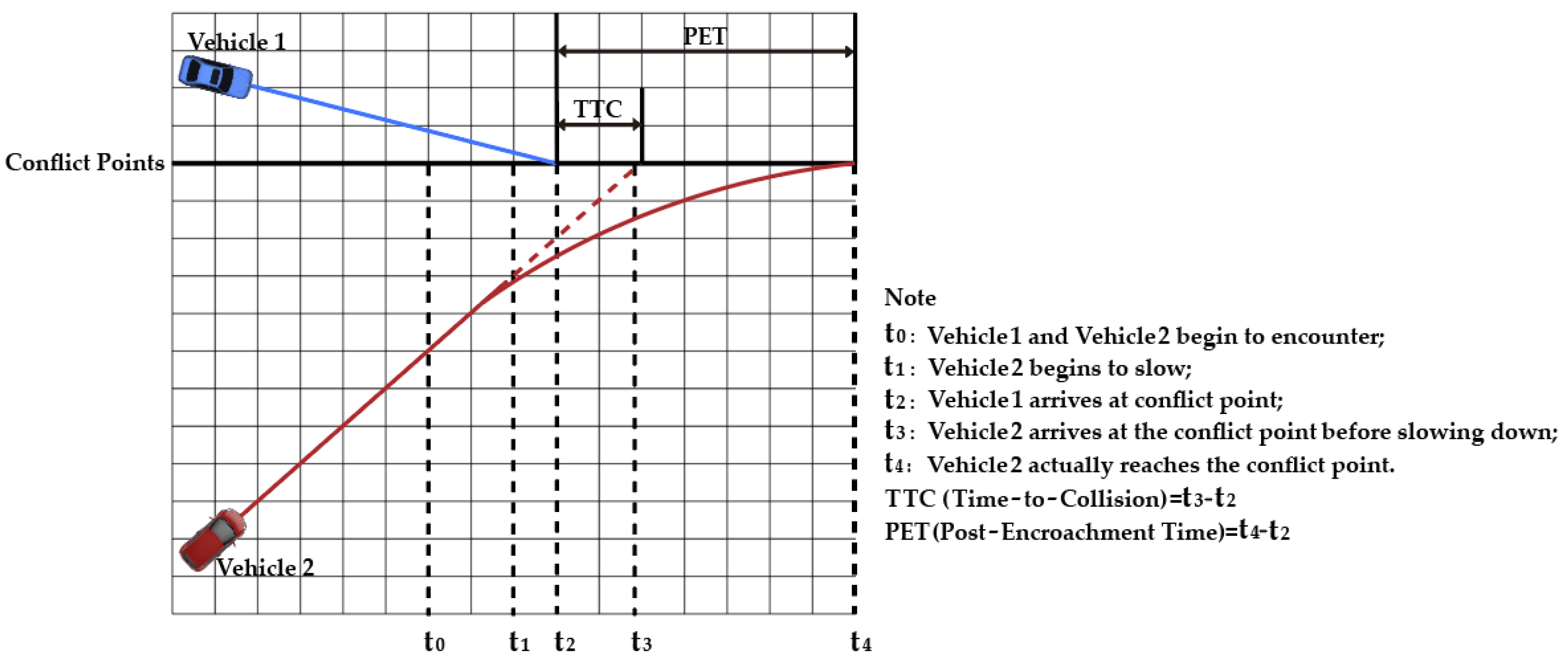
In order to accurately identify traffic conflict and select the most representative conflict parameters, the process of conflict occurrence needs to be analyzed. The occurrence process of traffic conflict is shown in Figure 4.
At moment t 0 , Vehicle 1 enters the conflict area, continues driving normally, and reaches the conflict point at moment t 2 . At moment t 1 , Vehicle 2 observes that, if it maintains its original driving speed and trajectory, it will reach the conflict point at moment t 3 , and the time gap between t 3 and t 2 is too small to ensure that Vehicle 1 will pass the conflict point; thus, it would collide with Vehicle 1. Therefore, Vehicle 2 starts to take risk-avoidance measures. At moment t 4 , Vehicle 2, which has taken risk-avoidance measures, reaches the conflict point, and Vehicle 1 has obtained enough of a time gap ( t 4 t 2 ) to pass the conflict point; thus, no collision occurs.
As seen from Figure 3, if Vehicle 2 is traveling at its original speed, the time difference between its arrival at the conflict point and that of Vehicle 1’s arrival will be too small to ensure the passage of the following vehicle, thus causing Vehicle 2 to take risk-avoidance measures. This time difference is defined as the Time-to-Collision (TTC). The time difference between Vehicle 1 and Vehicle 2 passing the conflict point after Vehicle 2 takes the risk-avoidance measures is defined as the Post-Encroachment Time (PET). The TTC and PET are calculated as follows.
TTC = t 3 t 2
PET = t 4 t 2
Suppose the coordinates of the intersection points on the trajectories of Vehicle 1 and Vehicle 2 at moments t 1 , t 2 , t 3 , t 4 are ( x A i , y A i ) , ( x B i , y B i ) , and the speed and acceleration of vehicles are V A i , V B i ; a A i , a B i , respectively, meaning that:
DeltaS = V A i V B i
maxD = max ( a A i ) , i = 1 , 2 , 3 , when   Vehicle   2   is   the   front   vehicle max ( a B i ) , i = 1 , 2 , 3 , when   Vehicle   1   is   the   front   vehicle
According to Equations (3) and (4), DeltaS is the difference in vehicle speeds as observed at TTC. More precisely, this value is mathematically defined as the magnitude of the difference in vehicle velocities (or trajectories). Consider an example where both vehicles are traveling at the same speed v . If they are traveling in the same direction, DeltaS = 0. If they have a perpendicular crossing path, DeltaS = 2 v . If they are approaching each other head on, DeltaS = 2 v . As opposed to DeltaS, MaxS is the maximum speed of either vehicle throughout the conflict (i.e., while the TTC is less than the specified threshold). MaxD is the maximum deceleration of the front vehicle. A negative value indicates deceleration (braking or release of the gas pedal). A positive value indicates that the vehicle did not decelerate during the conflict.
In addition, this paper also introduced the Probability of Unsuccessful Evasive Action for vehicles, i.e., P(UEA), which is obtained by the following two procedures:
  • From the initial positions and velocities of Vehicle 1 and Vehicle 2, 100 paths for each vehicle are generated using combinations of acceleration and orientation that are independently generated from two triangular distribution functions;
  • All collision points between every pair of projected paths are detected. P(UEA) is the percentage resulting from dividing the number of collision points by the total number of combinations of paths, that is:
    P ( UEA ) = C V e h 1 , V e h 2 P V e h 1 , V e h 2
    where C V e h 1 , V e h 2 represents all collision points between each pair of predicted paths for Vehicle 1 and Vehicle 2. P V e h 1 , V e h 2 represents the total number of path combinations between Vehicle 1 and Vehicle 2. P(UEA) can not only identify the conflicts that have occurred, but can also show the potential conflicts between vehicles, which has positive implications for traffic safety management and the prevention of traffic accidents.
The conflict angle division method in the SSAM classifies the conflict between vehicles into cross conflict, lane-change conflict, and rear-end conflict. Among them, cross-conflict refers to the type of conflict where the conflict angle of the vehicles is greater than 85°, which generally exists in road intersections. Since the experiment’s subject is urban expressways and no intersection exists, this paper did not consider cross conflict. Only rear-end conflict (0°, 30°) and lane-change conflict (30°, 85°) are considered. In addition, this paper selected vehicle state indicators, such as TTC, PET, MaxS, DeltaS, and MaxD, and vehicle conflict parameters, such as conflict angle, conflict type, and P(UEA), to study the influence of LSVs on traffic safety characteristics at 10 km/h on expressways. According to Ref. [45], the TTC threshold value was set as 1.5 s, the PET as 5 s, the rear-end conflict limit angle was 30°, and the cross-conflict angle was set as 80°.

4. Results

4.1. Vehicle Queuing and Dissipation Characteristics

4.1.1. Simulation with No LSVs

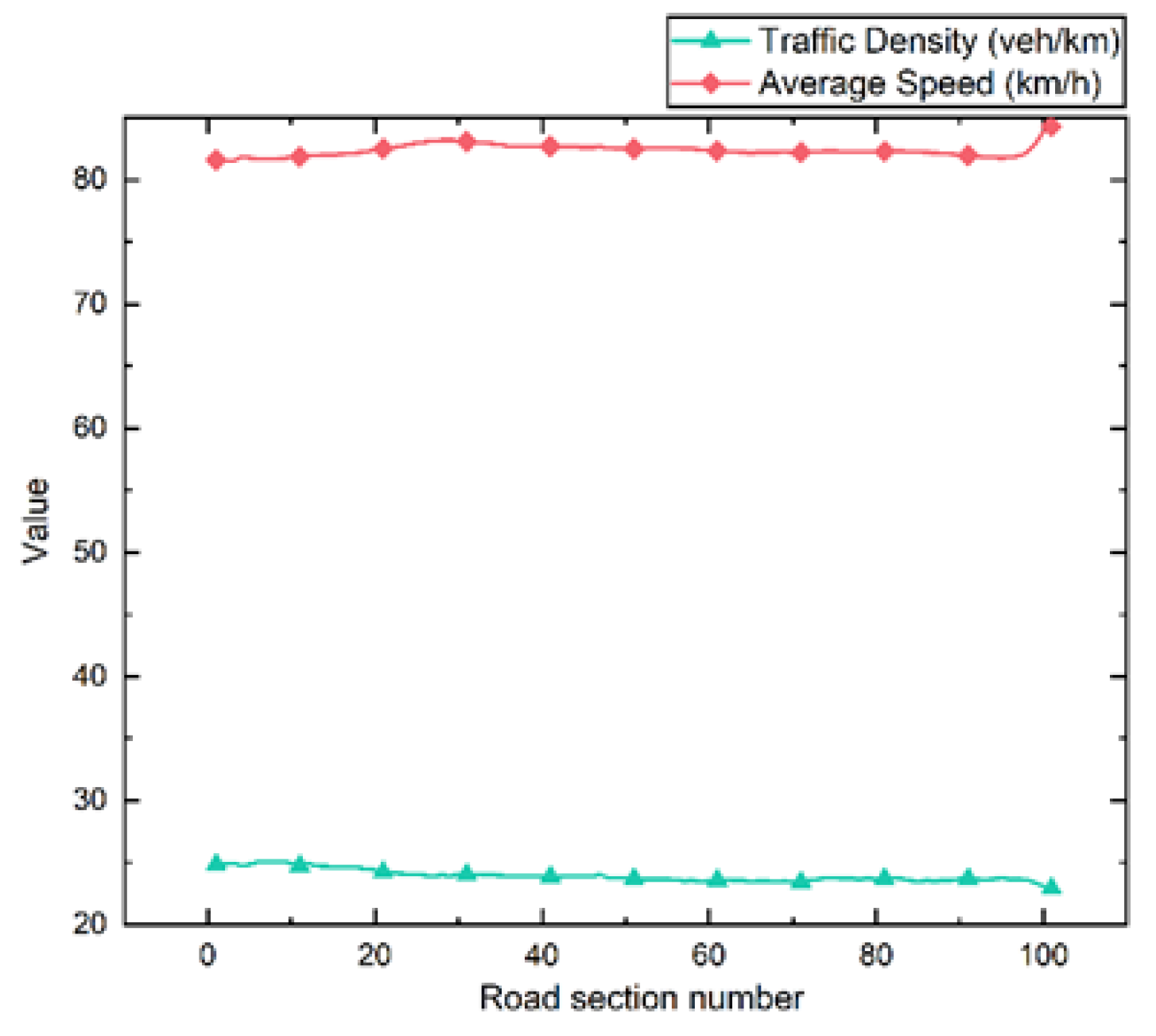
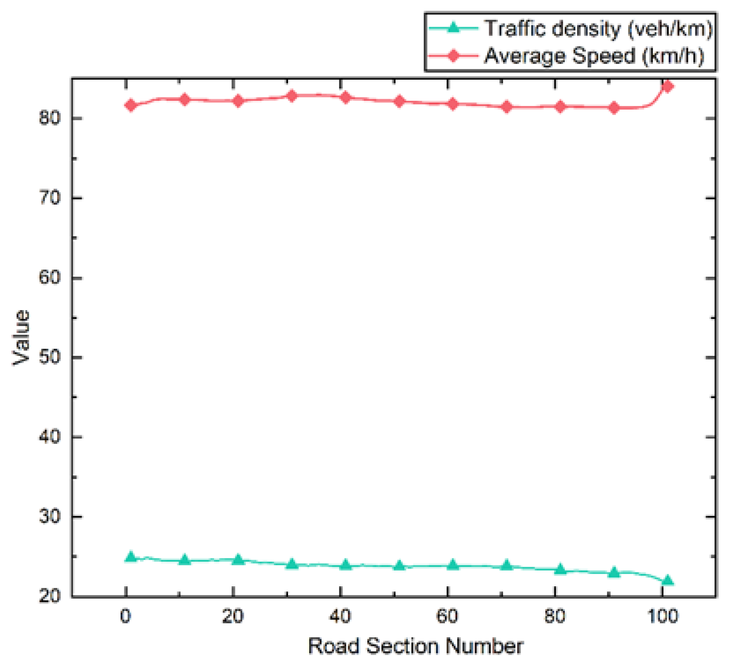
To investigate the influence of LSVs on expressway traffic flow, the conditions of expressway traffic flow were compared with and without LSVs. Based on the field data, the traffic density and average speed of each section of the three lanes without LSVs are shown in Figure 5, Figure 6 and Figure 7.
As seen in Figure 5, Figure 6 and Figure 7, the traffic density and average speed of each section do not vary much across different lanes. Among them, traffic density is maintained in the range of 20–30 vehicles/km, and average speed is maintained at around 80 km/h. In the actual driving environment, the inner lane is used for vehicle overtaking, so the average speed will be relatively high; the outer lane is generally used as an emergency lane, so the average speed is lower. However, the traffic simulation model in this experiment has traffic input values at the junction of peak and off-peak periods for the road section, so the vehicles are mostly in a free-running state and lane changes are not frequent. Therefore, although there is a difference in values for traffic density and average speed between the three lanes, the difference is not significant. In addition, due to the traffic volume of each road section not reaching capacity, drivers can enjoy a good driving experience, apart from accelerating and decelerating during short periods when entering or exiting the expressway. Currently, the road section service level is high, and no vehicle queuing occurs.

4.1.2. Simulation with LSVs

Previous studies have shown that LSVs significantly impact the vehicles that are following in the same lane [23]. Therefore, the following two hypotheses are proposed when LSVs exist on expressway sections:
  • Compared to a typical driving environment, LSVs will significantly affect road traffic flow due to speed differences with other vehicles. At this time, other vehicles will frequently accelerate, decelerate, or change lanes, causing large fluctuations in the road section’s average traffic density and speed;
  • Due to the unique characteristics of LSVs, the vehicles behind them will generate a backlog in a specific area on the road and form a queue, which begins to dissipate when the LSVs gradually move off the expressway.
To verify the above hypothesis, this paper used polynomial fitting to build a spatial evolution model of traffic density and average speed to study vehicle queuing and dissipation characteristics under the influence of LSVs.
When Speed of the LSV is Set at 10 km/h
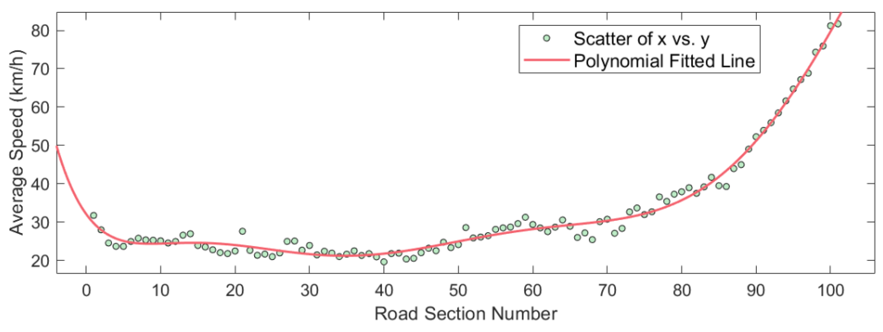
The speed of the LSV was set to 10 km/h and was moving in the outer lane. Figure 8 and Figure 9 show the variation graphs of traffic density and average speed for each section of the outer lane.
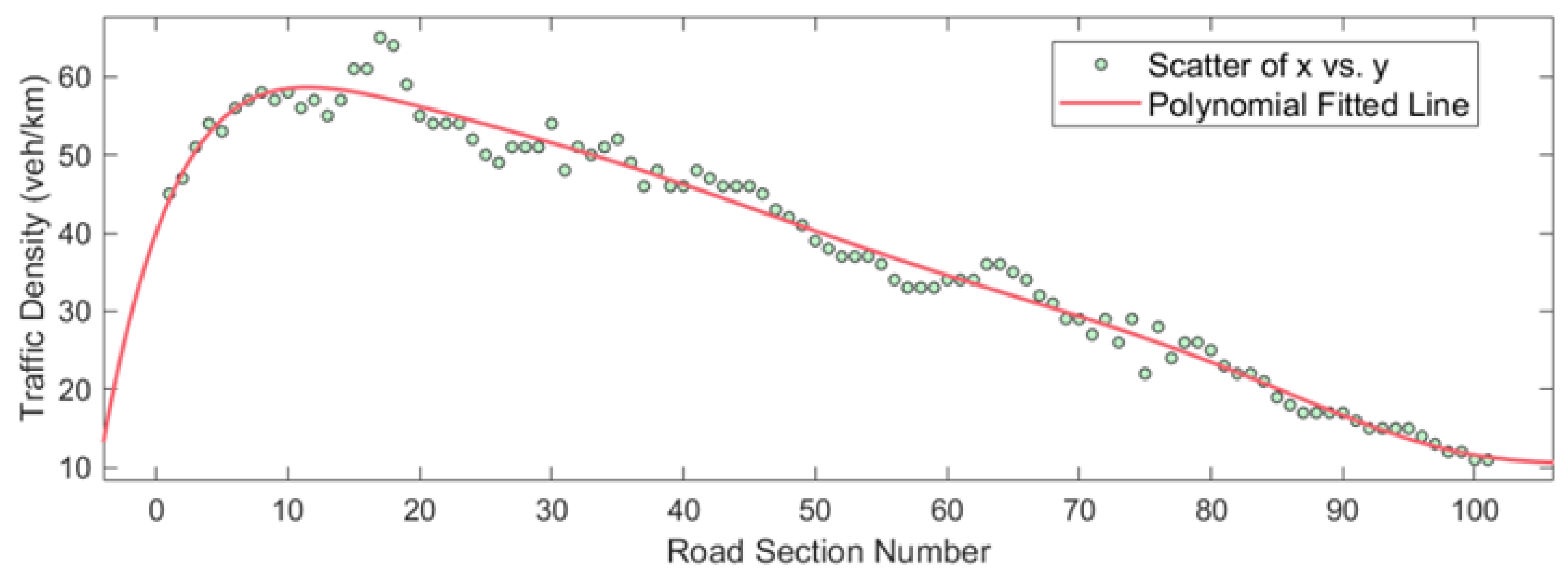
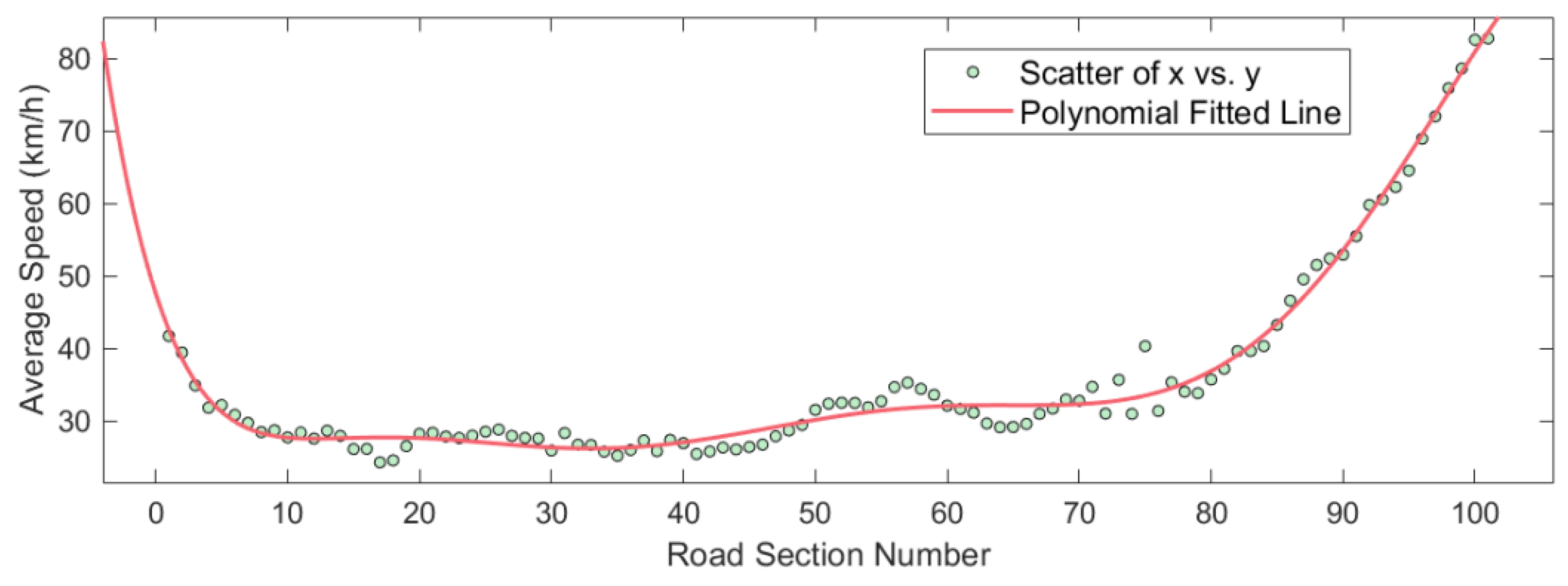
As shown in Figure 8 and Figure 9, when the LSV drives in the outer lane at 10 km/h, traffic density increases from the entrance of the road section. Furthermore, in Section 4, which is 30–40 m from the expressway entrance, traffic density reaches a peak of 69 vehicles/km. The average speed of this section is 23.65 km/h, indicating that vehicles are gradually backlogged at this time. Following that, in section 40, which is 390–400 m from the entrance of the expressway, although traffic density decreases, the average speed of the 40th section displays an overall downward trend, reducing to 19.60 km/h, which is 75.5%. lower than the section speed limit value. This indicates that the number of vehicles in the queue has reached the maximum and that vehicles need to follow behind the LSV at a low speed until there is a gap to change lanes. Subsequently, as the LSV moves forward, the overall density of each section of the outer lane further decreases and the average speed increases, indicating that the queue of vehicles is gradually dissipating.
In summary, traffic flow is unstable due to the lane and speed adjustment required for vehicles entering the expressway. Therefore, at the entrance of the road section, the LSV constitutes a sizeable negative impact on other vehicles and gradually creates a queue behind it. With the increasing traffic volume in the road section, the vehicles driving behind the LSV continue accumulating and are forced to slow down and follow until a traversable gap in the adjacent lane becomes available for a lane change. Since the input traffic volume does not reach roadway design capacity, the vehicles following the LSV can find a gap to change lanes within a certain period. Therefore, the vehicles driving behind the LSV will choose to change lanes to overtake the LSV, and the convoy gradually dissipates.
Using polynomial fitting to model the spatial evolution characteristics of traffic density and average speed with the LSV driving at 10 km/h, it was found that the spatial evolutionary trends of traffic density and average speed all satisfy the octet polynomial rule. The equation describing traffic density distribution dynamics is:
K 10 = 2.76 x 8 + 1.41 x 7 + 16.37 x 6 7.23 x 5 31.14 x 4 + 11.98 x 3 + 18.28 x 2 23.28 x + 39.47
The equation describing average speed dynamics distribution is:
V 10 = 0.63 x 8 1.87 x 7 3.68 x 6 + 10.61 x 5 + 9.83 x 4 13.38 x 3 2.30 x 2 + 10.82 x + 25.31
where K 10 and V 10 represent the traffic density and average speed under the 10 km/h LSV speed, respectively, with x representing the road section number. Through polynomial fitting, the R2 of the fitted traffic density distribution is 0.9802 and the R2 of the fitted average vehicle speed distribution is 0.9862, indicating an excellent fitting effect.
When the Speed of the LSV is Set at 15 km/h
The speed of the LSV was set to 15 km/h. Figure 10 and Figure 11 show the variation graphs of traffic density and average speed for each section of the outer lane.
As observed in Figure 10 and Figure 11, when the LSV moves in the outer lane at 15 km/h, the traffic density of the 17th section (160–170 m from the opening of the road section) reaches a peak of 65 vehicles/km, and the average speed reaches a minimum of 24.31 km/h. Subsequently, the average speed of the road section increases but the value is still low, indicating that vehicles are still queuing and that the number of vehicles in the queue is decreasing. Until section 41 (400–410 m from the entrance of the road section), average speed gradually increases, and congestion steadily eases. Figure 10 and Figure 11 also indicate that LSVs significantly impact other vehicles at the roadway entrance. As the speed of LSVs increases, the negative impact is even more powerful.
Using polynomial fitting to model the spatial evolution characteristics of traffic density and average speed with the LSV driving at 15 km/h, it was found that the spatial evolutionary trends of traffic density and average speed all satisfy the octet polynomial rule. The equation describing traffic density distribution dynamics is:
K 15 = 0.50 x 8 + 1.06 x 7 + 2.06 x 6 3.44 x 5 3.81 x 4 + 3.65 x 3 + 1.93 x 2 17.34 x + 39.67
The equation describing average speed dynamics distribution is:
V 15 = 0.90 x 8 2.74 x 7 5.19 x 6 + 13.27 x 5 + 14.02 x 4 14.21 x 3 7.85 x 2 + 8.53 x + 30.48
where K 15 and V 15 represent the traffic density and average speed under the 15 km/h LSV speed, respectively, with x representing the road section number. Using polynomial fitting, the R2 of the fitted traffic density distribution is 0.9816 and the R2 of the fitted average vehicle speed distribution is 0.9851, indicating an excellent fitting effect.
When the Speed of the LSV is Set at 20 km/h
The speed of the LSV was set to 20 km/h. Figure 12 and Figure 13 show the variation graphs of traffic density and average speed for each section of the outer lane.
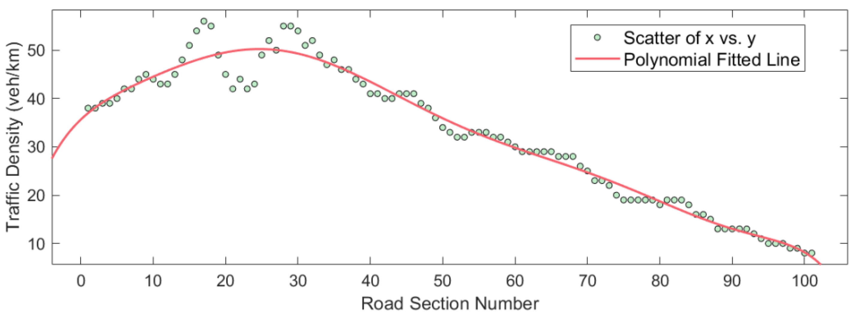
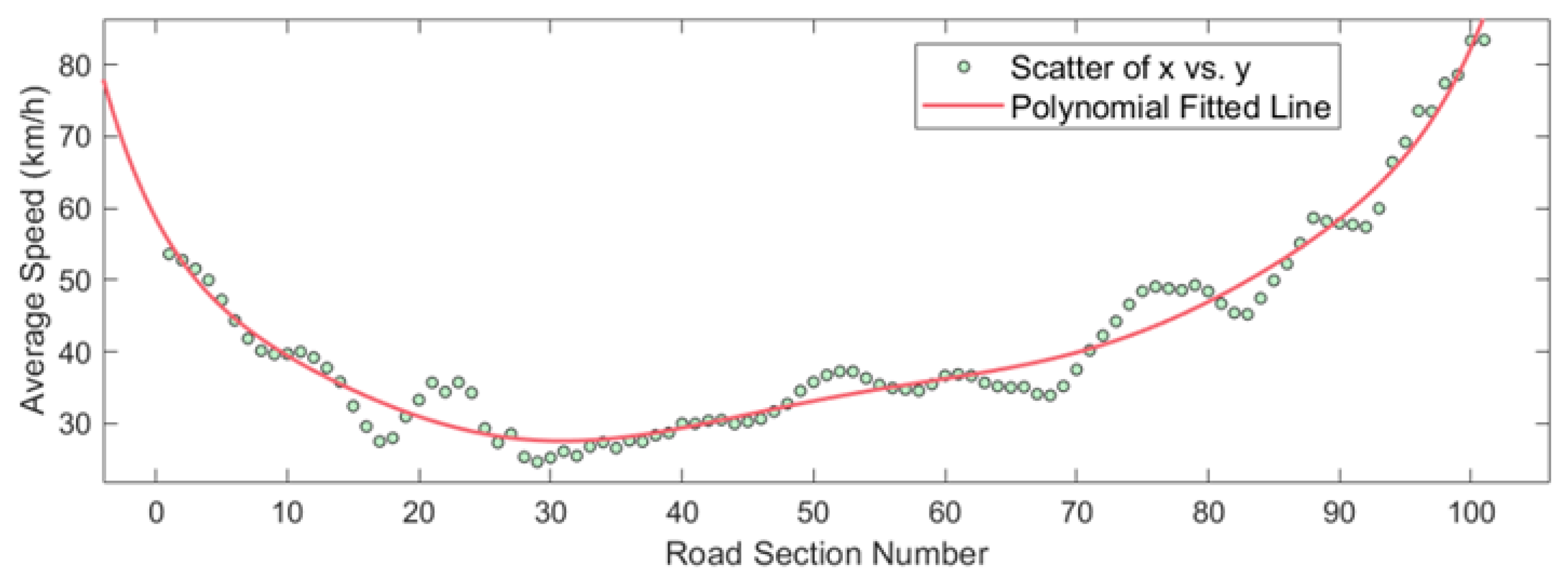
As demonstrated in Figure 12 and Figure 13, when the LSV drives in the outer lane of the expressway at 20 km/h, the traffic density of the 17th section (160–170 m from the entrance of the road section) reaches a peak of 56 vehicles/km, and the average speed of the section at this time reduces to 27.49 km/h. In the 28th section (270–280 m from the entrance of the road section), traffic density reaches another peak of 55 vehicles/km and the average speed reaches a minimum of 25.22 km/h, indicating that, from the entrance of the section to 160–170 m, vehicles gradually form a queue. Subsequently, at 220–230 m, some vehicles choose to change lanes through gaps, at which time the traffic gradually thins out before then forming a queue again. The number of vehicles queuing reaches its maximum at 270–280 m. After that, the line slowly dissipates as the LSV moves forward.
When the LSV travels at 20 km/h, there is still a sizeable negative impact on other vehicles at the road entrance. Moreover, as the speed of the LSV increases, the negative effect on the vehicles behind further decreases.
Using polynomial fitting to model the spatial evolution characteristics of traffic density and average speed with the LSV driving at 20 km/h, it was found that the spatial evolutionary trends of traffic density and average speed also satisfy the octet polynomial rule. The equation describing traffic density distribution dynamics is:
K 20 = 0.89 x 8 0.22 x 7 + 6.06 x 6 + 0.63 x 5 14.53 x 4 + 4.03 x 3 + 8.38 x 2 20.14 x + 35.22
The equation describing average speed dynamics distribution is:
V 20 = 1.20 x 8 + 0.24 x 7 6.71 x 6 0.30 x 5 + 15.42 x 4 1.46 x 3 4.79 x 2 + 10.14 x + 33.48
where K 20 and V 20 represent the traffic density and average speed under the 20 km/h LSV speed, respectively, with x representing the road section number. Using polynomial fitting, the R2 of the fitted traffic density distribution is 0.9683 and the R2 of the fitted average vehicle speed distribution is 0.9643, indicating an excellent fitting effect.
Focusing on the spatial evolution characteristics of traffic density and average speed at different LSV driving speeds in each section of the outer lane, when the LSV moves at different speeds it poses a significant negative impact on vehicles within about 400 m of the entrance section. At this point, vehicles rapidly accumulate and form queues. Subsequently, vehicles can gradually change to adjacent lanes as traffic flow stabilizes and congestion gradually eases. In addition, as the speed of the LSV increases, the impact on other vehicles diminishes, which verifies the correctness of the above two hypotheses. Through polynomial fitting, it is found that the evolutionary characteristics of traffic density and average speed for the outer lanes satisfy the octuple polynomial rule when an LSV travels at different speeds, reflecting the spatial heterogeneity of vehicle distribution at different LSV driving speeds.
The evolutionary expressions for traffic density and average speed at different LSV speeds are compiled in Table 1 and Table 2, respectively.
In the framework of traffic flow theory, traffic density is inversely related to average speed. Table 1 and Table 2 show that the coefficients of the evolutionary expressions of traffic density and average speed have opposite signs at different LSV speeds. Therefore, the above expressions are reasonable and convincing.
Among them, the ordinary equation describing the evolutionary characteristics of the outer lane’s traffic density at different LSV speeds is:
K = a 1 x 8 ± b 1 x 7 ± c 1 x 6 ± d 1 x 5 ± e 1 x 4 ± f 1 x 3 ± g 1 x 2 ± h 1 x + i 1
where a 1 , b 1 , c 1 , d 1 , e 1 , f 1 , g 1 , h 1 are the coefficients and i 1 is the constant term.
The ordinary equation describing the evolutionary characteristics of the outer lane’s average speed at different LSV speeds is:
V = a 2 x 8 b 2 x 7 c 2 x 6 d 2 x 5 e 2 x 4 f 2 x 3 g 2 x 2 h 2 x + i 2
where a 2 , b 2 , c 2 , d 2 , e 2 , f 2 , g 2 , h 2 are the coefficients and i 2 is the constant term.

4.2. Traffic Safety Characteristics Influenced by LSVs on Expressways

Section 4.1 mainly focuses on the effect of an LSV traveling in the same lane at different speeds on the behavior of other vehicles. In this section, the LSV’s driving speed is controlled constantly, and the differences in operational efficiency and traffic safety for the three lanes are analyzed through a comprehensive evaluation of the expressway surrogate risk indicators when an LSV drives in different lanes. As seen from Table 3, since the design speed of the inner lane is the greatest, when an LSV travels in the inner lane, the vehicles that are following need to slow down significantly and are prone to traffic conflicts. Therefore, the total number of conflicts in the inner lane is the largest and decreases sequentially from the inner lane to the outer lane. Generally, drivers will pass on the left side of the front vehicle during the lane change, but when the LSV travels on the inner lane, drivers have to pass the LSV on the right side. At this time, some drivers will follow the LSV instead of choosing to change lanes due to the restricted view. As a result, the number of rear-end conflicts is three times greater than the number of lane-change conflicts when the LSV travels in the middle lane. Due to the increased traffic flow, drivers driving behind the LSV cannot find a suitable gap to change lanes and thus decide to follow the LSV, increasing the probability of rear-end conflicts. In addition, When an LSV is driving in the outer lane, most drivers will change lanes to overtake the LSV due to the better view, so the number of lane-change conflicts in the outer lane is the highest.
In summary, when the LSV travels in different lanes at the same speed, the inner, middle, and outer lanes have the highest number of total conflicts, rear-end conflicts, and lane-change conflicts, respectively.
As seen in Table 4, the TTC and PET of the road sections do not change significantly when an LSV travels in different lanes, and the TTC values are within the interval [0, 1.5]. The threshold of TTC in the SSAM model is set as 1.5 s. This indicates that when the LSV is driving in the three lanes, some vehicles are judged to be in conflict because the TTC value is less than 1.5 s. In addition, the value of MaxD is negative for all three lanes, indicating that vehicles in all three lanes acted to slow down when traffic conflict occurred. As can be seen from the mean values of MaxD, the vehicles in the middle lane have the most significant speed reduction, indicating that the middle lane has the highest efficiency and that the vehicles are least affected by the LSV; however, the improvement is not significant. The smallest MaxD value for the outer lane represents the minor speed reduction that vehicles undertake when traffic conflicts occur, thus the vehicles in the outer lane are most affected by LSVs.
When the TTC is less than the threshold value, the MaxS of the middle lane is the largest, which is 47.9% higher than that of the outer lane. This indicates that the vehicles in the middle lane travel at the highest speed during traffic conflicts. Additionally, the variation magnitude of DeltaS shows that the vehicles in the middle lane have the most significant speed difference during traffic conflicts, which is 60.5% higher than that of the outer lane. From the above finding, it is clear that vehicles in the outer lane are the most affected by LSVs and they have the lowest traffic efficiency, while vehicles in the middle lane are the least affected and have the highest traffic efficiency. This finding is consistent with the variation characteristics of MaxD.
It is worth noting that the middle lane has the largest P(UEA) value among the three lanes, indicating that vehicles in the middle lane have the highest probability of potential traffic conflicts. P(UEA) is the ratio of the total number of conflict points to the number of path combinations among the 100 possible routes for two vehicles. Since the middle lane may be affected by the combined effect of vehicles in the inner and outside lanes, the potential risk is the greatest, although the middle lane is least affected by the LSV and has the highest throughput efficiency.

5. Discussion

5.1. Theoretical and Practical Applications

This paper investigates the mechanisms of LSVs’ influence on expressway traffic flow and traffic safety based on field data. Based on the results of the influence range of LSVs [26], this paper focuses on vehicle group behavior to explore the maximum influence range generated by LSVs on road sections. In addition, Ref. [46] took the speed and traffic volume of LSVs into account when studying the queue length and delay characteristics of vehicles under the influence of LSVs and obtained the speed–flow curves of road sections. Based on this, this paper focuses on vehicles’ queuing and dissipation behavior as the entry point for studying the influence mechanism of LSVs on other vehicles in the road section and investigates the impact range of LSVs on expressways. To achieve the above objectives, this study constructs a spatial evolution model of traffic density and average speed under different LSV speeds with the help of microscopic traffic simulation technology. The results show that the negative impact posed by LSVs is most significant within 400 m of the entrance to the expressway section and that the speed of the LSV is inversely proportional to the degree of impact. In addition, this study finds that the evolutionary characteristics of traffic density and average speed at different LSV speeds satisfy the octuple polynomial model, reflecting the spatial heterogeneity of vehicle distribution at different LSV driving speeds. At the application level, the octuple polynomial model obtained in this paper can be used to understand the distribution characteristics of vehicles in the lanes where LSVs travel and to grasp the sections with the most severe vehicle queuing phenomenon. These can then be used to adopt corresponding control strategies to reduce the driving risks of traffic accidents.
Using traffic conflict techniques, this paper constructs an SSAM-based model under the influence of LSVs and further explores the differences in vehicle conflicts in the corresponding lanes when an LSV drives in different lanes at the same speed. The results show that when the LSV drives in different lanes separately, the inner, middle, and outer lanes have the highest number of total conflicts, rear-end conflicts, and lane change conflicts, respectively. In addition, according to the comprehensive analysis of surrogate conflict indicators, vehicles in the outer lane are the most significantly affected by LSVs, while vehicles in the middle lane are the least affected and have the highest traffic efficiency; the MaxS and DeltaS are 47.9% and 60.5% higher than those of the outer lane, respectively. Nevertheless, vehicles in the middle lane have the highest probability of potential traffic conflicts. Ref. [27] explored the impact of LSVs on road traffic accident risk using actual road network measurement data, and their results are consistent with this paper. Based on the findings of this paper, road traffic management can propose measures to reduce traffic conflicts and improve driving safety in relation to LSVs on expressways through lane traveling restrictions, traffic management, and road alignment design. For example, LSVs should be restricted from traveling in the inner lanes to avoid more traffic conflicts. Meanwhile, the speed of other vehicles should be strictly controlled when LSVs are traveling in the middle or outer lane in order to avoid rear-end or lane-change conflicts. There are many ways to control the speed of vehicles, such as setting up variable information boards to control the minimum and maximum speed of LSVs. For special roads, such as urban tunnel entrance and exit sections, variable lane displacements can be set, based on the findings of Ref. [47], to plan the driving trajectory of LSVs so as to avoid traffic accidents.

5.2. Limitations and Future Research Directions

This paper discusses the impact of LSVs (which are common on roads and travel at speeds of 10–20 km/h) on the operation of expressway traffic flow and traffic safety. The conclusions obtained are applicable to traffic planning and the management of expressways. However, it remains to be investigated whether the findings drawn in this paper on the impact of LSVs on expressway traffic flow still apply to LSVs at higher speeds, such as those in the speed range of 20 km/h–40 km/h. Therefore, our future aim is to improve the scope of LSVs by further considering the performance of vehicles, driving behavior, and the driving environment. For example, the speed of moving work zones and some breakdown vehicles is generally 5–20 km/h, while vehicles with their speed steeply reduced due to driver distraction and trucks may also be defined as LSVs. Among them, trucks, as large vehicles, travel at speeds greater than 20 km/h but are still significantly different from those of small vehicles. Therefore, whether all of the possible LSVs mentioned above have the same influence mechanism on traffic flow and traffic safety, and whether a speed limit range can be proposed so as to apply to all LSVs, still needs further study. In addition, this study mainly takes a single LSV as the research object to study its impact on expressway traffic flow and traffic safety through microscopic traffic simulation. In the actual road traffic environment, more attention should be paid to the road traffic volume of LSVs. Measuring the coupled driving risk caused by multiple LSVs is an unsolved problem. In addition, although this experiment is based on a field investigation, the simulation model may still differ from the actual traffic operation environment due to errors in data collection. With the help of driving simulators, eye-tracking devices, and other equipment, combining drivers’ physiological and psychological characteristics under actual road traffic conditions with the empirical data is also the goal of our continuous studies in the future. Meanwhile, with the emergence of autonomous vehicles (AVs), more and more studies are focusing on the traffic flow state when AVs are mixed with human-driven vehicles. In this paper, only the interaction behavior between human-driven vehicles is considered. In the future, it is important to consider LSVs as AVs in order to study their impact on the traffic safety of expressways.

6. Conclusions

In this paper, the following conclusions are drawn from the simulation and analysis of LSVs on expressways:
  • The evolutionary features of lane traffic density and average speed under different LSV speeds satisfy the octuple polynomial law, reflecting the spatial heterogeneity of vehicle distribution at different LSV driving speeds;
  • LSVs with varying speeds have the most significant negative impact on the road section within 400 m of the expressway entrance, and the lower the speed of the LSV, the more substantial the impact produced;
  • When an LSV drives in different lanes separately, the inner, middle, and outer lanes have the highest number of total conflicts, rear-end conflicts, and lane-change conflicts, respectively. In addition, vehicles in the outer lane are the most significantly affected by LSVs, while vehicles in the middle lane are the least affected and have the highest traffic efficiency; MaxS and DeltaS for the middle lane are 47.9% and 60.5% higher than those of the outer lane, respectively. Nevertheless, the middle lane has the highest probability of potential traffic conflicts.

Author Contributions

Conceptualization, C.X. and J.M.; methodology, C.X.; software, C.X.; validation, C.X; formal analysis, X.T.; investigation, J.M.; resources, C.X.; data curation, C.X.; writing—original draft preparation, C.X.; writing—review and editing, X.T.; visualization, C.X.; supervision, J.M.; project administration, C.X.; funding acquisition, J.M. All authors have read and agreed to the published version of the manuscript.

Funding

This research was supported by the Transportation Science and Technology Project of Jiangsu Province (Jianxiao Ma, Grant No. 2018Y15).

Institutional Review Board Statement

Not applicable.

Informed Consent Statement

Not applicable.

Data Availability Statement

Data are available from the corresponding author upon reasonable request.

Conflicts of Interest

The authors declare no conflict of interest.

References

  1. Gazis, D.C. The moving and ‘phantom’ bottlenecks. Transp. Sci. 1992, 26, 223–229. [Google Scholar] [CrossRef]
  2. Newell, G.F. A moving bottleneck. Transp. Res. Pt. B-Methodol. 1998, 32, 531–537. [Google Scholar] [CrossRef]
  3. Wang, C.; Zhong, M.; Zhang, H.; Li, S.Y. Impacts of real-time traffic state on urban expressway crashes by collision and vehicle type. Sustainability 2022, 14, 2238. [Google Scholar] [CrossRef]
  4. Tian, Y.J.; Xiao, D.L.; Wang, L.; Chen, H. Expressway traffic safety early warning system based on cloud architecture. Comput. Commun. 2021, 171, 140–147. [Google Scholar] [CrossRef]
  5. Jin, S.; Qu, X.B.; Wang, D.H. Assessment of expressway traffic safety using gaussian mixture model based on time to collision. Int. J. Comput. Intell. Syst. 2011, 4, 1122–1130. [Google Scholar]
  6. Qu, Q.K.; Chen, F.J.; Zhou, X.J. Road traffic bottleneck analysis for expressway for safety under disaster events using blockchain machine learning. Saf. Sci. 2019, 118, 925–932. [Google Scholar] [CrossRef]
  7. Shi, Q.; Abdel-Aty, M. Evaluation of the impact of travel time reliability on urban expressway traffic safety. Transp. Res. Record. 2016, 2582, 8–17. [Google Scholar] [CrossRef]
  8. Sun, J.; Li, T.N.; Li, F.; Chen, F. Analysis of safety factors for urban expressways considering the effect of congestion in Shanghai, China. Accid. Anal. Prev. 2016, 95, 503–511. [Google Scholar] [CrossRef]
  9. Ma, Y.F.; Meng, H.C.; Chen, S.Y.; Zhao, J.G.; Li, S.; Xiang, Q.J. Predicting traffic conflicts for expressway diverging areas using vehicle trajectory data. J. Transp. Eng. Pt. A-Syst. 2020, 146, 04020003. [Google Scholar] [CrossRef]
  10. Fadhloun, K.; Rakha, H.; Loulizi, A. Impact of underlying steady-state fundamental diagram on moving bottleneck passing rates using a second-order traffic model. Transp. Lett. 2014, 6, 185–196. [Google Scholar] [CrossRef]
  11. Hunter-Zaworski, K.M. Impacts of low-speed vehicles on transportation infrastructure and safety. J. Transp. Land Use 2012, 5, 68–76. [Google Scholar] [CrossRef] [Green Version]
  12. Zhang, H.; Li, S.Y.; Wu, C.Z.; Zhang, Q.; Wang, Y.F. Predicting crash frequency for urban expressway considering collision types using real-time traffic data. J. Adv. Transp. 2020, 2020, 1–8. [Google Scholar] [CrossRef]
  13. Zhao, J.B.; Deng, W. Traffic accidents on expressways: New threat to China. Traffic Inj. Prev. 2012, 13, 230–238. [Google Scholar] [CrossRef]
  14. Liang, G.H.; Sun, X.J.; Zhang, Y.D.; Chen, M.L.; Zhang, W.T. Identifying expressway accident black spots based on the secondary division of road units. Promet.-Traffic Transp. 2021, 33, 731–743. [Google Scholar] [CrossRef]
  15. Jia, B.; Jiang, R.; Wu, Q.S.; Hu, M.B. Honk effect in the two-lane cellular automaton model for traffic flow. Physica A. 2005, 348, 544–552. [Google Scholar] [CrossRef]
  16. Klenov, S.L.; Wegerle, D.; Kerner, B.S.; Schreckenberg, M. Prediction of moving and unexpected motionless bottlenecks based on three-phase traffic theory. Comput. Res. Modeling 2021, 13, 319–363. [Google Scholar] [CrossRef]
  17. Hu, X.J.; Lin, C.X.; Hao, X.T.; Lu, R.Y.; Liu, T.H. Influence of tidal lane on traffic breakdown and spatiotemporal congested patterns at moving bottleneck in the framework of Kerner’s three-phase traffic theory. Physics A 2021, 584, 126335. [Google Scholar] [CrossRef]
  18. Wegerle, D.; Kerner, B.S.; Schreckenberg, M.; Klenov, S.L. Prediction of moving bottleneck through the use of probe vehicles: A simulation approach in the framework of three-phase traffic theory. J. Intell. Transport. Syst. 2020, 24, 598–616. [Google Scholar] [CrossRef]
  19. Kerner, B.S.; Klenov, S.L. A theory of traffic congestion at moving bottlenecks. J. Phys. A Math. Theor. 2010, 43, 425101. [Google Scholar] [CrossRef]
  20. Lighthill, M.J.; Whitham, J.B. On kinematic waves II. A theory of traffic flow on long crowded roads. Proc. R. Soc. Lond. 1955, 53, 275–354. [Google Scholar]
  21. Wei, X.Y.; Xu, C.C.; Wang, W.; Yang, M.L.; Ren, X.L. Evaluation of average travel delay caused by moving bottlenecks on highways. PLoS ONE 2017, 12, e0183442. [Google Scholar] [CrossRef] [PubMed]
  22. Simoni, M.D.; Claudel, C.G. A fast simulation algorithm for multiple moving bottlenecks and applications in urban freight traffic management. Transp. Res. Pt. B-Methodol. 2017, 104, 238–255. [Google Scholar] [CrossRef]
  23. Daganzo, C.F.; Laval, J.A. Moving bottlenecks: A numerical method that converges in flows. Transp. Res. Pt. B-Methodol. 2005, 39, 855–863. [Google Scholar] [CrossRef]
  24. Daganzo, C.F.; Laval, J.A. On the numerical treatment of moving bottleneck. Transp. Res. Pt. B-Methodol. 2005, 39, 31–46. [Google Scholar] [CrossRef]
  25. Fang, S.; Ma, J.X. Influence range and traffic risk analysis of moving work zones on urban roads. Sustainability 2021, 13, 4196. [Google Scholar] [CrossRef]
  26. Gan, X.F.; Weng, J.X.; Zhang, J. Evaluation of travel delay and accident risk at moving work zones. J. Transp. Saf. Secur. 2021, 13, 622–641. [Google Scholar] [CrossRef]
  27. Yang, Y.; Tian, N.; Wang, Y.P.; Yuan, Z.Z. A Parallel FP-Growth Mining Algorithm with Load Balancing Constraints for Traffic Crash Data. Int. J. Comput. Commun. Control 2022, 17, 4806. [Google Scholar] [CrossRef]
  28. Yang, Y.; Yuan, Z.Z.; Meng, R. Exploring Traffic Crash Occurrence Mechanism toward Cross-Area Freeways via an Improved Data Mining Approach. J. Transp. Eng. Pt. A-Syst. 2022, 148, 04022052. [Google Scholar] [CrossRef]
  29. Yang, Y.; He, K.; Wang, Y.P.; Yuan, Z.Z.; Yin, Y.H.; Guo, M.Z. Identification of dynamic traffic crash risk for cross-area freeways based on statistical and machine learning methods. Physica A 2022, 595, 127083. [Google Scholar] [CrossRef]
  30. Yang, Y.; Wang, K.; Yuan, Z.Z.; Liu, D. Predicting Freeway Traffic Crash Severity Using XGBoost-Bayesian Network Model with Consideration of Features Interaction. J. Adv. Transp. 2022, 2022, 4257865. [Google Scholar] [CrossRef]
  31. Yao, Z.Z.; Hu, R.; Jiang, Y.S.; Xu, T.R. Stability and safety evaluation of mixed traffic flow with connected automated vehicles on expressways. J. Saf. Res. 2020, 75, 262–274. [Google Scholar] [CrossRef] [PubMed]
  32. Yu, R.J.; Wang, Y.Y.; Quddus, M.; Li, J.; Wang, X.S.; Tian, Y. Investigating vehicle roadway usage patterns on the Shanghai urban expressway system and their impacts on traffic safety. Int. J. Sustain. Transp. 2021, 15, 217–228. [Google Scholar] [CrossRef]
  33. Oskarbski, J.; Kaminski, T.; Kyamakya, K.; Chedjou, J.C.; Zarski, K.; Pedzierska, M. Assessment of the Speed Management Impact on Road Traffic Safety on the Sections of Motorways and Expressways Using Simulation Methods. Sensors 2020, 20, 5057. [Google Scholar] [CrossRef] [PubMed]
  34. Wang, X.F.; Li, X.W.; Yan, Y.; Fu, X.S. Driving Risk Affected Areas and Distribution Function of Sharp Horizontal Curves of Expressway. Discrete Dyn. Nat. Soc. 2015, 2015, 208564. [Google Scholar] [CrossRef]
  35. Yu, R.J.; Wang, X.S.; Yang, K.; Abdel-Aty, M. A Hybrid Latent Class Analysis Modeling Approach to Analyze Urban Expressway Crash Risk. Accid. Anal. Prev. 2017, 101, 37–43. [Google Scholar] [CrossRef] [PubMed]
  36. Wang, L.; Abdel-Aty, M.; Lee, J. Safety analytics for integrating crash frequency and real-time risk modeling for expressways. Accid. Anal. Prev. 2017, 104, 58–64. [Google Scholar] [CrossRef]
  37. Yang, K.; Wang, X.S.; Yu, R.J. A Bayesian dynamic updating approach for urban expressway real-time crash risk evaluation. Transp. Res. Pt. C-Emerg. Technol. 2013, 51, 252–259. [Google Scholar] [CrossRef]
  38. Wang, J.H.; Kong, Y.M.; Fu, T. Expressway crash risk prediction using back propagation neural network: A brief investigation on safety resilience. Accid. Anal. Prev. 2019, 124, 180–192. [Google Scholar] [CrossRef]
  39. Wang, L.N. Real-Time Evaluation Method of Vehicle Conflict Risk on Urban Expressway Based on Smartphone GPS Data. J. Adv. Transp. 2021, 2021, 2407529. [Google Scholar] [CrossRef]
  40. Charly, A.; Mathew, T.V. Evaluation of driving performance in relation to safety on an expressway using field driving data. Transp. Lett. 2020, 12, 340–348. [Google Scholar] [CrossRef]
  41. Rahman, M.S.; Abdel-Aty, M. Longitudinal safety evaluation of connected vehicles’ platooning on expressways. Accid. Anal. Prev. 2018, 117, 381–391. [Google Scholar] [CrossRef]
  42. Qi, W.W.; Wang, Z.X.; Tang, R.R.; Wang, L.H. Driving risk detection model of deceleration zone in expressway based on generalized regression neural network. J. Adv. Transp. 2018, 2018, 8014385. [Google Scholar] [CrossRef]
  43. Zhang, C.; Wang, B.; Yang, S.X.; Zhang, M.; Gong, Q.L.; Zhang, H. The driving risk analysis and evaluation in rightward zone of expressway reconstruction and extension engineering. J. Adv. Transp. 2020, 2020, 8943463. [Google Scholar] [CrossRef]
  44. Jiang, Y.; Zhang, J.Y.; Wang, Y.H.; Wang, W.Y. Drivers’ behavioral responses to driving risk diagnosis and real-time warning information provision on expressways: A smartphone app-based driving experiment. J. Transp. Saf. Secur. 2020, 12, 329–357. [Google Scholar] [CrossRef]
  45. Balakrishna, R.; Antoniou, C.; Ben-Akiva, M.; Koutsopoulos, H.N.; Wen, Y. Calibration of Microscopic Traffic Simulation Models: Methods and Application. Transp. Res. Rec. 2007, 1999, 198–207. [Google Scholar] [CrossRef]
  46. Chitturi, M.V.; Benekohal, R.F. Work zone queue length and delay methodology. Transp. Lett. 2010, 2, 273–283. [Google Scholar] [CrossRef]
  47. Fang, S.; Shen, L.H.; Ma, J.X.; Xu, C.B. Study on the Design of Variable Lane Demarcation in Urban Tunnels. Sustainability 2022, 14, 5682. [Google Scholar] [CrossRef]
Figure 1. Lane positions of the road section. The number “1” refers to the low-speed vehicles.
Sustainability 14 12165 g001
Figure 2. Road section division.
Sustainability 14 12165 g002
Figure 3. SSAM model workflow.
Sustainability 14 12165 g003
Figure 4. Traffic conflict trajectories of Vehicle 1 and Vehicle 2.
Sustainability 14 12165 g004
Figure 5. Traffic density and average speed of each section of the outer lane without LSVs.
Sustainability 14 12165 g005
Figure 6. Traffic density and average speed of each section of the middle lane without LSVs.
Sustainability 14 12165 g006
Figure 7. Traffic density and average speed of each section of the inner lane without LSVs.
Sustainability 14 12165 g007
Figure 8. Variation graphs of traffic density with the LSV driving at 10 km/h.
Sustainability 14 12165 g008
Figure 9. Variation graphs of average speed with the LSV driving at 10 km/h.
Sustainability 14 12165 g009
Figure 10. Variation graphs of traffic density with the LSV driving at 15 km/h.
Sustainability 14 12165 g010
Figure 11. Variation graphs of average speed with the LSV driving at 15 km/h.
Sustainability 14 12165 g011
Figure 12. Variation graphs of traffic density with the LSV driving at 20 km/h.
Sustainability 14 12165 g012
Figure 13. Variation graphs of average speed with the LSV driving at 20 km/h.
Sustainability 14 12165 g013
Table 1. Comparison of traffic density expressions for different speeds of LSV.
Speed of LSVExpressions for Evolutionary Features
10 km/h K 10 = 2.76 x 8 + 1.41 x 7 + 16.37 x 6 7.23 x 5 31.14 x 4 + 11.98 x 3 + 18.28 x 2 23.28 x + 39.47
15 km/h K 15 = 0.50 x 8 + 1.06 x 7 + 2.06 x 6 3.44 x 5 3.81 x 4 + 3.65 x 3 + 1.93 x 2 17.34 x + 39.67
20 km/h K 20 = 0.89 x 8 0.22 x 7 + 6.06 x 6 + 0.63 x 5 14.53 x 4 + 4.03 x 3 + 8.38 x 2 20.14 x + 35.22
Table 2. Comparison of average speed expressions for different speeds of LSV.
Speed of LSVExpressions for Evolutionary Features
10 km/h V 10 = 0.63 x 8 1.87 x 7 3.68 x 6 + 10.61 x 5 + 9.83 x 4 13.38 x 3 2.30 x 2 + 10.82 x + 25.31
15 km/h V 15 = 0.90 x 8 2.74 x 7 5.19 x 6 + 13.27 x 5 + 14.02 x 4 14.21 x 3 7.85 x 2 + 8.53 x + 30.48
20 km/h V 20 = 1.20 x 8 + 0.24 x 7 6.71 x 6 0.30 x 5 + 15.42 x 4 1.46 x 3 4.79 x 2 + 10.14 x + 33.48
Table 3. Comparison of the number of conflicts in the SSAM model for the three lanes.
TotalCrossingRear-EndLane-Change
Inner Lane3402014
Middle Lane280235
Outer Lane2901415
Table 4. Descriptive statistics for the SSAM model parameters of the three lanes.
Conflict ParametersMinimumMaximumMean
InnerMiddleOuterInnerMiddleOuterInnerMiddleOuter
TTC0.00.00.01.51.51.51.11.10.8
PET0.00.00.04.64.23.62.11.91.5
MaxS2.93.73.119.122.722.110.210.87.3
MaxD−7.7−7.6−8.0−1.3−1.4−1.5−5.03−4.1−5.4
DeltaS0.50.30.115.418.112.66.56.94.3
P(UEA)0.00.00.00.81.00.90.20.30.2
Publisher’s Note: MDPI stays neutral with regard to jurisdictional claims in published maps and institutional affiliations.