Effects of Subsidy Cancellations on Investment Strategies of Local Governments and New Energy Vehicle Manufacturers: A Study Based on Differential Game

Abstract

The intensity of China’s new energy vehicle (NEV) subsidies has gradually declined since 2017 and is expected to end in the next few years, thereby causing market fluctuations and affecting the investment strategies of both local governments and automotive enterprises. In order to examine the effects of a subsidy cancellation, this study introduced it as an external disturbance to establish a differential game model, in which a random arrival process is used to represent the occurrence of a cancellation. The model incorporated both decentralized and centralized modes at the pre- and post-subsidy cancellation stages. A numerical simulation showed that the investments of both parties, the market demand, and the system benefits in both modes would be lower when compared to the scenario in which the subsidy is not canceled, but continued. The performance of the centralized mode was superior to that of the decentralized one, implying that the centralized mode was capable of realizing Pareto optimality. A sensitivity analysis of the model’s parameters showed that the timing of the subsidy cancellation would not affect the investment levels of either party in either stage, but losses of market demand and system benefits would occur shortly after the cancellation and continue until stabilizing.

1. Introduction

The development of the new energy vehicle (NEV) industry is an important pathway for China to guarantee strategic energy security while achieving green and sustainable economic growth. In order to promote the healthy development of the industry in its early stages, China launched a variety of tax incentives and subsidy policies for R&D, infrastructure, and consumption [1,2]. These subsidy policies have effectively improved the core technologies of the NEVs and cultivated the market [3]. According to the China Automobile Association [4], sales of NEVs exceeded 3.5 million vehicles in 2021 and the market share increased to 13.4%. The national strategy of “carbon peaking and carbon neutrality” [5,6] has accelerated vehicle electrification and promoted sales. In order to let the NEV industry strengthen itself, the subsidies at the national level have been gradually weakening since 2017 and are expected to be withdrawn in a few years. In order to eliminate the shock to the market demand caused by the subsidy reduction and to encourage automotive manufacturers to produce more NEVs, the Ministry of Industry and Information Technology jointly issued with other departments the “Measures for the Parallel Management of Average Fuel Consumption and New Energy Vehicle Points of Passenger Vehicle Enterprises,” or the fuel consumption dual-point policy [7], so that automotive enterprises could weigh the production ratio between traditional vehicles and NEVs for optimal benefits.

The implementation of a NEV subsidy policy always initiates a game between the government and enterprises due to their different roles and interests. Most studies have examined such a game by using an evolutionary game model. For example, Ref. [8] established a static mixed strategy evolutionary game model. In Ref. [9], the effects of subsidies on the R&D and introduction of NEV enterprises were evaluated. In Ref. [10], an indirect evolutionary game was introduced to examine the interactive relationships between the two players. In Ref. [11], the strategies of manufacturers in response to different combinations of carbon taxes and subsidies were analyzed. Moreover, Ref. [12] investigated fraudulent behaviors among NEV enterprises in response to subsidies.

The above-mentioned studies have mainly applied evolutionary game theory and mathematical models, as well as presented rational decisions for both the government and enterprises. However, these evolutionary game models are all placed in scenarios without quantitative considerations of external disturbances. Random factors or emergency events in the real world have non-negligible effects on the game participants. The adjustment of national macroeconomic policies can affect the local government and even the entire game, so neither game player would be able to accurately predict the timing of such events. Therefore, stochastic optimal control theory is necessary [13]. In Refs. [14,15], an optimal brand advertising strategy to handle product crises was formulated. The optimal decisions and profits of supply chain members were analyzed in Ref. [16] by considering random crises. In Ref. [17], a differential game model of suppliers and manufacturers for food safety crises was established. In Ref. [18], a differential game model to design the equilibrium strategies of two competing firms was developed, of which one or both could issue product recalls at any time. A stochastic differential game was used in Ref. [19] to study the optimal pricing strategy of company managers for product recall crises. In Ref. [20], an optimal advertising strategy for a supply chain faced with a potential brand crisis was proposed. Dynamic resource management for the risk of an abrupt change in the organizational environment was discussed in Ref. [21].

Although game theory applied to NEV subsidy policies has attracted many scholars, they have mainly applied evolutionary rather than differential game theory, and have not considered external disturbances such as subsidy cancellations, which are crises that could pose urgent problems to both local governments and enterprises. Differential game theory is based on differential equations and is capable of quantitatively incorporating external disturbances into a differential model, which is superior to an evolutionary game. To fill the research gap, this paper proposes an application of differential game theory to explore NEV subsidy policies. The main contribution of this study is its establishment of a differential game with the introduction of the element of uncertainty posed by a subsidy cancellation, which is described by a random arrival process. This paper discusses decentralized and centralized decision-making modes, as well as the numerical simulation and the sensitivity analysis of the parameters that have been conducted by this study. The organization of the remainder of this paper is as follows. Section 2 introduces a differential game model. Section 3 presents solutions to the model in both decentralized and centralized decision-making modes, then Section 4 compares the results of the solutions to other policy scenarios. Section 5 discusses the results of the numerical simulation and the sensitivity analysis of the parameters of the model. Finally, Section 6 presents the conclusions.

2. Problem Description and Differential Game Model

2.1. Problem Description

In the initial development stage of the NEV industry, the government usually takes many positive policy measures, such as tax reductions, to provide financial subsidies for the research and development. This is in order to cultivate the market and promote the healthy, rapid development of the NEV industry. However, in reality, with the aim of maximizing its benefit, an enterprise would smartly adjust its investment strategies for research and development according to the strength of NEV subsidy, and thus influence the level of updating NEV technology. At the nest stage, the government would readjust the strength of the NEV subsidy according to the technological level of the NEV, while the enterprises would also change their investment strategies in response to the new subsidy policy. Therefore, this game arises from the interactive decisions between the government and the enterprises. Capable of combining the conventional game theory and optimization methodology, differential game theory has been recognized as a typical mathematical tool for analyzing the decisions and behaviors with regard to the investment strategies of two players in a continuous time domain.

2.2. Model Assumptions

Proposition 1.

For a differential game between the local government and NEV enterprises, a subsidy cancellation policy was designed and formulated at the national level.

Proposition 2.

Two scenarios concerning the subsidy policy are discussed for comparison purposes. In Scenario 1, the subsidy is expected to be canceled, so the decision-making horizons of the local government and enterprise are divided into two stages: the first stage (before cancellation) and second stage (after cancellation). In Scenario 2, the subsidy is not canceled, but continued.

Proposition 3.

Let the investment of the NEV enterprises be $I_{Ei}\left(t\right)$, which is used for the technology upgrade and new product research. Let the investment of the local government be $I_{Gi}\left(t\right)$, which is used to publicize the advantages of NEVs to consumers and to subsidize a portion of the R&D costs of the enterprises. The market demand for NEVs is usually decided by many factors, such as the investment levels of both parties, the prices of NEVs, the structure of the market, and the nature of the subsidy policy. So, the market demand $Q\left(t\right)$ can be expressed as:

$$dQ\left(t\right)={\lambda }_{Ei}{I}_{Ei}\left(t\right)dt+{\lambda }_{Gi}{I}_{Gi}\left(t\right)dt-{\gamma }_i{P}_i-{\delta }_{i}Q\left(t\right)dt+\psi Q\left(t\right)q\left(t\right)$$

(1)

where $t$ is time, with the subscript $i$ = 1, 2 denoting the two respective stages representing the periods before and after the subsidy cancellation; ${\lambda }_{Ei}$ and ${\lambda }_{Gi}$ are the respective effect coefficients of the local government and enterprises on the market demand, whose natural decay rate is ${\delta }_i$; $P_i$ is the price of an NEV; ${\gamma }_i$ is the effect coefficient of the price on the market demand; $\psi$ is the loss rate of the market demand, which can be regarded as an independent and identically distributed random variable to describe the jump amplitude of the market demand; and $q\left(t\right)$ is a binary function that equals 1 in the case of a jump, but 0 in all other cases.

Proposition 4.

A subsidy cancellation will result in a loss of market demand. Let $Q\left(T^{-}\right)$ and $Q\left(T^{+}\right)$ denote the respective levels of market demand before and after the subsidy cancellation. Then, the change in market demand can be expressed as:

$$Q\left(T^{-}\right)-Q\left(T^{+}\right)=\psi Q\left(T^{-}\right),$$

(2)

The market demand cannot be negative, so $Q\left(T^{+}\right)=\left(1-\psi \right)Q\left(T^{-}\right)>0$, where $0<\psi <1$. Let $p\left(a\right)$ denote the probability density function of $\psi$, which conforms to a uniform distribution:

$$p\left(a\right)=\left\{\begin{array}{cc}1,\hfill & 0<\psi <1\\ 0,\hfill & \mathrm{else}\end{array}\right.$$

Proposition 5.

Before the subsidy cancellation, let the cost-sharing ratio of the government’s subsidy be $w\left(t\right).$ A quadratic function relation is used to describe the relationship between the investments and costs [22]. Then, the respective investment costs of an enterprise and the local government are:

$$C_E\left(I_{Ei}\right)=\frac{1}{2}{k}_E{I}_{Ei}^2\left(t\right)$$

$$C_G\left(I_{Gi}\right)=\frac{1}{2}{k}_G{I}_{Gi}^2\left(t\right),$$

where $C_E\left(·\right)$ and $C_G\left(·\right)$ are their respective cost functions while $k_E$ and $k_G$ are their respective cost coefficients.

Before the subsidy is canceled, the government shares part of the investment costs of the enterprise. Then, the respective cost functions of both parties in the first stage are:

$$C_E\left(I_{E1}\right)=\left(1-w\left(t\right)\right)\frac{1}{2}{k}_E{I}_{E1}^2\left(t\right)$$

$$C_G\left(I_{G1}\right)=\frac{1}{2}{k}_G{I}_{G1}^2\left(t\right)+\frac{1}{2}w{k}_E{I}_{E1}^2\left(t\right).$$

The marginal benefits of both parties will change after the cancellation. Thus, the benefits in each of the two stages (before and after the cancellation) must be calculated separately. In the first stage:

$$J_{E1}\left(I_{E1}\right)=\underset{I_{E1}}{max}{{\displaystyle \int }}_0^T{e}^{-\rho t}[{\alpha }_{E1}Q\left(t\right)+{\beta }_{d1}{I}_{E1}-C_E\left(I_{E1}\right)] dt$$

$$J_{G1}\left(I_{G1}\right)=\underset{I_{G1}}{max}{{\displaystyle \int }}_0^T{e}^{-\rho t}[{\alpha }_{G1}Q\left(t\right)+{\beta }_{j1}{I}_{E1}-C_G\left(I_{G1}\right)] dt$$

In the second stage:

$$J_{E2}\left(I_{E2}\right)=\underset{I_{E2}}{max}{{\displaystyle \int }}_T^{\infty }{e}^{-\rho \left(t-T\right)}[{\alpha }_{E2}Q\left(t\right)+{\beta }_{d2}{I}_{E2}-C_E\left(I_{E2}\right)] dt$$

$$J_{G2}\left(I_{G2}\right)=\underset{I_{G2}}{max}{{\displaystyle \int }}_T^{\infty }{e}^{-\rho \left(t-T\right)}[{\alpha }_{G2}Q\left(t\right)+{\beta }_{j2}{I}_{E2}-C_G\left(I_{G2}\right)] dt$$

where $\rho$ is the discount rate, $J_{E1}$ and $J_{E2}$ are the enterprise’s respective benefits at the first and second stages, $T$ is the time of the cancellation, ${\alpha }_{E1}$ and ${\alpha }_{E2}$ are the respective marginal benefit coefficients of the enterprise’s investment for the two stages, ${\alpha }_{G1}$ and ${\alpha }_{G2}$ are the respective marginal benefit coefficients of the government’s investment, ${\beta }_{d1}$ and ${\beta }_{d2}$ are the benefit coefficients of the government’s fuel consumption dual-point policy, and ${\beta }_{j1}$ and ${\beta }_{j2}$ are the influence coefficients of the enterprise’s investment on the government’s indirect social benefits, such as environmental improvement. By producing more NEVs, the enterprise can obtain more fuel consumption points, which can be exchanged for benefits on the national exchange platform.

The respective total benefits of the local government and enterprise for both stages are:

$$J_E\left(I_{E1},I_{E2}\right)=J_{E1}\left(I_{E1}\right)+e^{-\rho T}{J}_{E2}\left(I_{E2}\right)$$

$$J_G\left(I_{G1},I_{G2}\right)=J_{G1}\left(I_{G1}\right)+e^{-\rho T}{J}_{G2}\left(I_{G2}\right)$$

For a clear and concise presentation, four propositions about the differential game model are summarized in Figure 1.

2.3. Game Model Construction

The subsidy can be canceled at any time $T$, which can therefore be considered a random variable [14]. $\left\{\Gamma \left(t\right),t\ge 0\right\}$ is a Poisson process with the parameter $x$. If $x=1$, then the cancellation would occur at some point in the future. The event $\left\{T>t\right\}$ occurs if and only if the Poisson event does not occur in [0, t]. For $t\ge 0$:

$$P\left\{T>t\right\}=P\left\{\Gamma \left(t\right)=0\right\}=\frac{{(xt)}^0}{0!}{e}^{-xt}=e^{-xt}$$

(3)

Then, the probability distribution function of $T$ is

$$F_T\left(t\right)=\left\{\begin{array}{cc}1-e^{-xt},& t\ge 0\\ 0,& t<0\end{array}\right.$$

and the probability density function of $T$ is

$$f_t\left(t\right)={\dot{F}}_T\left(t\right)=\left\{\begin{array}{cc}x{e}^{-xt},& t\ge 0\\ 0,& t<0\end{array}\right.$$

(4)

The expected net present values of both the government and enterprises, respectively, can be obtained by calculating the mathematical expectations for all possible $T$ over both stages:

$$J_E\left(I_{E1},I_{E2}\right)=E\left[J_{E1}\left(I_{E1}\right)+e^{-\rho T}{J}_{E2}\left(I_{E2}\right)\right]$$

(5a)

$$J_G\left(I_{G1},I_{G2}\right)=E\left[J_{G1}\left(I_{G1}\right)+e^{-\rho T}{J}_{G2}\left(I_{G2}\right)\right]$$

(5b)

Equation (5a,b) can be further expressed as:

$$\begin{array}{ll}{J}_E\left(I_{E1},I_{E2}\right)& ={{\displaystyle \int }}_0^{\infty }{e}^{-\left(\rho +x\right)t}\left[{\alpha }_{E1}Q\left(t\right)+{\beta }_{d1}{I}_{E1}-C_E\left(I_{E1}\right)\right]dt+x{{\displaystyle \int }}_0^{\infty }{e}^{-\left(\rho +x\right)t}{J}_{E2}\left(I_{E2}\right)dt\\ & ={{\displaystyle \int }}_0^{\infty }{e}^{-\left(\rho +x\right)t}\{{\displaystyle \left[{\alpha }_{E1}Q\left(t\right)+{\beta }_{d1}{I}_{E1}-C_E\left(I_{E1}\right)\right]}+x{J}_{E2}\left(I_{E2}\right)\}dt\end{array}$$

(6a)

$$\begin{array}{ll}{J}_G\left(I_{G1},I_{G2}\right)& ={{\displaystyle \int }}_0^{\infty }{e}^{-\left(\rho +x\right)t}\left[{\alpha }_{G1}Q\left(t\right)+{\beta }_{j1}{I}_{E1}-C_G\left(I_{G1}\right)\right]dt+x{{\displaystyle \int }}_0^{\infty }{e}^{-\left(\rho +x\right)t}{J}_{G2}\left(I_{G2}\right)dt\\ & ={{\displaystyle \int }}_0^{\infty }{e}^{-\left(\rho +x\right)t}\{\left[{\alpha }_{G1}Q\left(t\right)+{\beta }_{j1}{I}_{E1}-C_G\left(I_{G1}\right)\right]+x{J}_{G2}\left(I_{G2}\right)\}dt\end{array}$$

(6b)

The derivation of Equation (6a) is:

$$\begin{array}{ll}{J}_E\left(I_{E1},I_{E2}\right)& =E[{{\displaystyle \int }}_0^t{e}^{-\rho s}[{\alpha }_{E1}Q\left(s\right)+{\beta }_{d1}{I}_{E1}-C_E\left(I_{E1}\right)] ds+e^{-\rho t}{J}_{E2}\left(I_{E2}\right)]\\ & ={{\displaystyle \int }}_0^{\infty }\{{{\displaystyle \int }}_0^t{e}^{-\rho s}[{\alpha }_{E1}Q\left(s\right)+{\beta }_{d1}{I}_{E1}-C_E\left(I_{E1}\right)] ds+e^{-\rho t}{J}_{E2}\left(I_{E2}\right)\}\left(x{e}^{-xt}\right)dt\\ & ={{\displaystyle \int }}_0^{\infty }\{{{\displaystyle \int }}_0^t{e}^{-ps}\left[{\alpha }_{E1}Q\left(s\right)+{\beta }_{d1}{I}_{E1}-C_E\left(I_{E1}\right)\right] ds\}\left(x{e}^{-xt}\right)dt+x{{\displaystyle \int }}_0^{\infty }{e}^{-\left(\rho +x\right)t}{J}_{E2}\left(I_{E2}\right)dt\end{array}$$

because

$$\begin{array}{c}{\int }_0^{\infty }\{{\int }_0^t{e}^{-ps}\left[{\alpha }_{E1}Q\left(s\right)+{\beta }_{d1}{I}_{E1}-C_E\left(I_{E1}\right)\right] ds\}\left(x{e}^{-xt}\right)dt=\left[-e^{-xt}U\left(t\right)\right]\left|{ }_0^{\infty }\right.-{\int }_0^{\infty }\left(-e^{-xt}\right)(e^{-\rho t}[{\alpha }_{E1}Q\left(s\right)+\\ {\beta }_{d1}{I}_{E1}-C_E\left(I_{E1}\right)]dt={\int }_0^{\infty }{e}^{-\left(\rho +x\right)t}\left[{\alpha }_{E1}Q\left(s\right)+{\beta }_{d1}{I}_{E1}-C_E\left(I_{E1}\right)\right] dt.\end{array}$$

Equation (6b) can be similarly derived.

3. Solution to Differential Game Model

This section discusses the optimal strategies of the local government and enterprises with both decentralized and centralized game modes in anticipation of the subsidy cancellation. For convenience, the time variable t is omitted from the following formulas.

3.1. Decentralized Game Mode

In the decentralized game mode, also known as the non-cooperative game mode (N-mode), each player aims to maximize their own interest. We assume that the local government shares part of the investment costs of the enterprise in the first stage, but no longer does so in the second stage. Thus, a government-led Stackelberg differential game is formed in the first stage, but a common non-cooperative game is formed in the second stage.

Theorem 1.

In the decentralized game mode, the government’s optimal cost-sharing ratio, optimal investments of both parties in both stages, and the market demand are as follows:

$$w^N=\left\{\begin{array}{ll}\frac{{\lambda }_{E1}\left[\left(\rho +{\delta }_2\right)\left(2{\alpha }_{G1}-{\alpha }_{E1}\right)+\left(1-\psi \right)\left(2{\alpha }_{G2}-{\alpha }_{E2}\right)\right]+\left(\rho +{\delta }_2\right)\left(\rho +x+{\delta }_1\right)\left(2{\beta }_{j1}-{\beta }_{d1}\right)}{{\lambda }_{E1}\left[\left(\rho +{\delta }_2\right)\left(2{\alpha }_{G1}+{\alpha }_{E1}\right)+\left(1-\psi \right)\left(2{\alpha }_{G2}+{\alpha }_{E2}\right)\right]+\left(\rho +{\delta }_2\right)\left(\rho +x+{\delta }_1\right)\left(2{\beta }_{j1}+{\beta }_{d1}\right)},& 2B>A\\ 0,& 2B\le A\end{array}\right.$$

$$I_{E1}^N=\left\{\begin{array}{c}\frac{{\lambda }_{E1}\left[{\alpha }_{E1}\left(\rho +{\delta }_2\right)+x\left(1-\psi \right){\alpha }_{E2}\right]+{\beta }_{d1}\left(\rho +x+{\delta }_1\right)\left(\rho +{\delta }_2\right)}{\left(1-w^N\right)k_E\left(\rho +x+{\delta }_1\right)\left(\rho +{\delta }_2\right)},2B>A\\ \frac{{\lambda }_{E1}\left[{\alpha }_{E1}\left(\rho +{\delta }_2\right)+x\left(1-\psi \right){\alpha }_{E2}\right]+{\beta }_{d1}\left(\rho +x+{\delta }_1\right)\left(\rho +{\delta }_2\right)}{k_E\left(\rho +x+{\delta }_1\right)\left(\rho +{\delta }_2\right)},2B\le A\end{array}\right.$$

$$I_{E2}^N=\frac{{\beta }_{d2}\left(\rho +{\delta }_2\right)+{\lambda }_{E2}{\alpha }_{E2}}{k_E\left(\rho +{\delta }_2\right)}$$

$$I_{G1}^N=\frac{{\lambda }_{G1}\left[{\alpha }_{G1}\left(\rho +{\delta }_2\right)+x\left(1-\psi \right){\alpha }_{G2}\right] }{k_G\left(\rho +x+{\delta }_1\right)\left(\rho +{\delta }_2\right)}$$

$$I_{G2}^N=\frac{{\lambda }_{G2}{\alpha }_{G2}}{k_G\left(\rho +{\delta }_2\right)}$$

$$Q^N\left(t\right)=\{\begin{array}{ll}{e}^{-{\delta }_{1}t}\left(Q_0-Q_{1RSS}^N\right)+Q_{1RSS}^N,\hfill & t\in \left[0,T\right]\hfill \\ e^{-{\delta }_2\left(t-T\right)}\left(Q_{T^{+}}^N-Q_{2RSS}^N\right)+Q_{2RSS}^N,\hfill & t\in \left(T,\infty \right)\hfill \end{array}$$

where the superscript $N$ denotes the non-cooperative game mode, $A={\beta }_{d1}+\frac{{\lambda }_{E1}\left[\left(1-\phi \right){\alpha }_{E2}+\left(\rho +{\delta }_2\right){\alpha }_{E1}\right]}{\left(\rho +{\delta }_2\right)\left(\rho +x+{\delta }_1\right)}$, $B={\beta }_{j1}+\frac{{\lambda }_{E1}\left[\left(1-\psi \right){\alpha }_{G2}+\left(\rho +{\delta }_2\right){\alpha }_{G1}\right]}{\left(\rho +{\delta }_2\right)\left(\rho +x+{\delta }_1\right)}$, $Q_{1RSS}^N=\frac{{\lambda }_{E1}{I}_{E1}^N+{\lambda }_{G1}{I}_{G1}^N-{\gamma }_1{P}_1}{{\delta }_1}$ and $Q_{2RSS}^N=\frac{{\lambda }_{E2}{I}_{E2}^N+{\lambda }_{G2}{I}_{G2}^N-{\gamma }_2{P}_2}{{\delta }_2}$ are the respective stable market demand in the first and second stages, and $Q_0$ and $Q_{T^{+}}^N=\left(1-\psi \right)\left[e^{-{\delta }_{1}T}\left(Q_0-Q_{1RSS}^N\right)+Q_{1RSS}^N\right]$ are the initial market demand in the first and second stages, respectively.

Proof of Theorem 1.

In the post-subsidy cancellation stage, the optimal value of the infinite boundary autonomous problem depends on the initial state and elapsed time [22], but is independent of the initial time. Therefore, the initial time in the second stage can be changed so that the optimal government and enterprise benefits can be expressed as follows:

$$J_{E2}\left(I_{E2}\right)=\underset{I_{E2}}{max}{{\displaystyle \int }}_0^{\infty }{e}^{-\rho t}[{\alpha }_{E2}Q\left(t\right)+{\beta }_{d2}{I}_{E2}-C_E\left(I_{E2}\right)] dt$$

$$J_{G2}\left(I_{G2}\right)=\underset{I_{G2}}{max}{{\displaystyle \int }}_0^{\infty }{e}^{-\rho t}[{\alpha }_{G2}Q\left(t\right)+{\beta }_{j2}{I}_{E2}-C_G\left(I_{G2}\right)] dt$$

According to the principle of reverse deduction, the optimization problem in the second stage can be solved first by using the form of a Hamilton–Jacobi–Bellman (HJB) equation [23]:

$$\rho V_{E2}^N\left(Q\left(T^{+}\right)\right)=\underset{I_{E2}}{max}\left\{{\alpha }_{E2}Q+{\beta }_{d2}{I}_{E2}\left(t\right)-\frac{1}{2}{k}_E{I}_{E2}{(t)}^2+{\dot{V}}_{E2}^N\left[{\lambda }_{E2}{I}_{E2}\left(t\right)+{\lambda }_{G2}{I}_{G2}\left(t\right)-{\delta }_{2}Q-{\gamma }_2{P}_2\right]\right\}$$

(7)

$$\rho V_{G2}^N\left(Q\left(T^{+}\right)\right)=\underset{I_{G2}}{max}\left\{{\alpha }_{G2}Q+{\beta }_{j2}{I}_{E2}-\frac{1}{2}{k}_G{I}_{G2}{(t)}^2+{\dot{V}}_{G2}^N\left[{\lambda }_{E2}{I}_{E2}\left(t\right)+{\lambda }_{G2}{I}_{G2}\left(t\right)-{\delta }_{2}Q-{\gamma }_2{P}_2\right]\right\},$$

(8)

where ${\dot{V}}_{E2}^N=\frac{\partial V_{E2}^N}{\partial Q}$ and ${\dot{V}}_{G2}^N=\frac{\partial V_{G2}^N}{\partial Q}$ are the current optimal benefit functions of the enterprise and government, respectively. □

Differentiating Equations (7) and (8) with respect to $I_{E2}$ and $I_{G2}$, then setting to zero:

$$I_{E2}=\frac{{\beta }_{d2}+{\lambda }_{E2}{\dot{V}}_{E2}^N}{k_E}$$

(9)

$$I_{G2}=\frac{{\lambda }_{G2}{\dot{V}}_{G2}^N}{k_G}$$

(10)

Substituting Equations (9) and (10) into Equations (7) and (8), respectively:

$$\rho V_{E2}^N\left(Q\left(T^{+}\right)\right)=({\alpha }_{E2}-{\delta }_2{\dot{V}}_{E2}^N)Q+\frac{{({\beta }_{d2}+{\lambda }_{E2}{\dot{V}}_{E2}^N)}^2}{2k_E}+\frac{{\lambda }_{G2}{}^2{\dot{V}}_{E2}^N{\dot{V}}_{G2}^N}{k_G}-{\dot{V}}_{E2}^N{\gamma }_2{P}_2$$

(11)

$$\rho V_{G2}^N\left(Q\left(T^{+}\right)\right)=({\alpha }_{G2}-{\delta }_2{\dot{V}}_{G2}^N)Q+\frac{{({\lambda }_{G2}{\dot{V}}_{G2}^N)}^2}{2k_G}+\frac{{\beta }_{j2}{\beta }_{d2}+{\beta }_{j2}{\lambda }_{E2}{\dot{V}}_{E2}^N+{\beta }_{d2}{\lambda }_{E2}{\dot{V}}_{G2}^N+{\lambda }_{E2}{}^2{\dot{V}}_{E2}^N{\dot{V}}_{G2}^N}{k_E}-{\dot{V}}_{G2}^N{\gamma }_2{P}_2$$

(12)

Therefore, the form of the optimal current benefit function can be set as:

$$V_{E2}^N\left(Q\left(T^{+}\right)\right)=m_{1}Q+l_1$$

(13)

$$V_{G2}^N\left(Q\left(T^{+}\right)\right)=m_{2}Q+l_2$$

(14)

then,

$$V_{E2}^N{}^{\prime }=m_1$$

(15a)

$$V_{G2}^N{}^{\prime }=m_2$$

(15b)

Comparing the coefficients of the same terms in Equations (11) and (12) with Equations (13) and (14), respectively:

$$m_1=\frac{{\alpha }_{E2}}{\rho +{\delta }_2}$$

(16a)

$$m_2=\frac{{\alpha }_{G2}}{\rho +{\delta }_2}$$

(16b)

$$l_1=\frac{1}{\rho }\left[\frac{{({\beta }_{d2}+{\lambda }_{E2}{m}_1)}^2}{2k_E}+\frac{{\lambda }_{G2}{}^2{m}_1{m}_2}{k_G}-m_1{\gamma }_2{P}_2\right]$$

$$l_2=\frac{1}{\rho }[\frac{{({\lambda }_{G2}{m}_2)}^2}{2k_G}+\frac{{\beta }_{j2}{\beta }_{d2}+{\beta }_{j2}{\lambda }_{E2}{m}_1+{\beta }_{d2}{\lambda }_{E2}{m}_2+{\lambda }_{E2}{}^2{m}_1{m}_2}{k_E}-m_2{\gamma }_2{P}_2]$$

Substituting Equations (15) and (16) into Equations (9) and (10), respectively, the respective optimal investments of local government and enterprise can be calculated by:

$$I_{E2}^N=\frac{{\beta }_{d2}\left(\rho +{\delta }_2\right)+{\lambda }_{E2}{\alpha }_{E2}}{k_E\left(\rho +{\delta }_2\right)}$$

$$I_{G2}^N=\frac{{\lambda }_{G2}{\alpha }_{G2}}{k_G\left(\rho +{\delta }_2\right)}$$

Substituting Equations (2), (13), and (14) into Equation (6), the respective benefits of the local government and enterprises in both stages can be obtained:

$$J_E\left(I_{E1},I_{E2}\right)=\underset{I_{E1},I_{E2}}{max}{{\displaystyle \int }}_0^{\infty }{e}^{-\left(p+x\right)t}[{\alpha }_{E1}Q\left(t\right)+{\beta }_{d1}{I}_{E1}-C_E\left(I_{E1}\right)]+V_{E2}^N\left(G\left(T^{+}\right)\right)\}dt$$

$$J_G\left(I_{G1},I_{G2}\right)=\underset{I_{G1},I_{G2}}{max}{{\displaystyle \int }}_0^{\infty }{e}^{-\left(p+x\right)t}[{\alpha }_{G1}Q\left(t\right)+{\beta }_{j1}{I}_{E1}-C_G\left(I_{G1}\right)]+V_{G2}^N\left(G\left(T^{+}\right)\right)\}dt$$

In the first stage, the government shares part of the enterprise’s investment costs to form a government-led Stackelberg differential game. In this game mode, the government first decides its own investment and the cost-sharing ratio. Then, the enterprise decides according to the government’s decisions.

The optimal control problem in the first stage can be solved first by using the HJB form of the optimal benefit function:

$$\begin{array}{cc}\hfill \left(\rho +x\right)V_{E1}^N\left(Q\right)=& \underset{I_{E1}}{max}\left\{{\alpha }_{E1},Q,+,{\beta }_{d1},I_{E1},\left(t\right),-,\left(1-w\right),\frac{1}{2},k_E,I_{E1},{(t)}^2,+,m_1,\left(1-\psi \right),Q,+,l_1,+,{\dot{V}}_{E1}^N,[,{\lambda }_{E1},I_{E1},\left(t\right)\right.\hfill \\ & \left.+,{\lambda }_{G1},I_{G1},\left(t\right),-,{\delta }_1,Q,-,{\gamma }_1,P_1,]\right\}\hfill \end{array}$$

(17)

Differentiating Equation (17) with respect to $I_{E1}$ and setting to zero:

$$I_{E1}=\frac{{\beta }_{d1}+{\lambda }_{E1}{\dot{V}}_{E1}^N}{\left(1-w\right)k_E},$$

(18)

where ${\dot{V}}_{E1}^N=\frac{\partial V_{E1}^N}{\partial Q}$.

In order to maximize its benefit, a rational government would predict the enterprise’s level of investment. The government’s HJB equation can be expressed as:

$$\begin{array}{ll}\left(\rho +x\right)V_{G1}^N\left(Q\right)=& \underset{I_{G1}}{max}\{{\alpha }_{G1}Q+{\beta }_{j1}{I}_{E1}\left(t\right)-\frac{1}{2}{k}_G{I}_{G1}{(t)}^2-w\frac{1}{2}{k}_E{I}_{E1}{(t)}^2+m_2\left(1-\psi \right)Q+l_2+{\dot{V}}_{G1}^N[{\lambda }_{E1}{I}_{E1}\left(t\right)\\ & +{\lambda }_{G1}{I}_{G1}\left(t\right)-{\delta }_{1}Q-{\gamma }_1{P}_1]{\displaystyle \}}\end{array}$$

(19)

Substituting Equation (18) into Equation (19):

$$\begin{array}{ll}\left(\rho +x\right)V_{G1}^N\left(Q\right)=& \underset{I_{G1}}{max}\{{\alpha }_{G1}Q+{\beta }_{j1}\frac{{\beta }_{d1}+{\lambda }_{E1}{\dot{V}}_{E1}^N}{\left(1-w\right)k_E}-\frac{1}{2}{k}_G{I}_{G1}{(t)}^2-w\frac{1}{2}{k}_E[\frac{{\beta }_{d1}+{\lambda }_{E1}{\dot{V}}_{E1}^N}{\left(1-w\right)k_E}]{ }^2+m_2\left(1-\psi \right)Q+l_2\\ & +{\dot{V}}_{G1}^N[{\lambda }_{E1}\frac{{\beta }_{d1}+{\lambda }_{E1}{\dot{V}}_{E1}^N}{\left(1-w\right)k_E}+{\lambda }_{G1}{I}_{G1}\left(t\right)-{\delta }_{1}Q-{\gamma }_1{P}_1]\}\end{array}$$

(20)

Differentiating Equation (20) with respect to $I_{G1}$ and $w$, then setting to zero:

$$I_{G1}=\frac{{\lambda }_{G1}{\dot{V}}_{G1}^N}{k_G}$$

(21)

$$w=\{\begin{array}{ll}\frac{2\left({\beta }_{j1}+{\dot{V}}_{G1}^N{\lambda }_{E1}\right)-\left({\beta }_{d1}+{\dot{V}}_{E1}^N{\lambda }_{E1}\right)}{2\left({\beta }_{j1}+{\dot{V}}_{G1}^N{\lambda }_{E1}\right)+\left({\beta }_{d1}+{\dot{V}}_{E1}^N{\lambda }_{E1}\right)},& 2B>A\\ 0,& 2B\le A\end{array}$$

(22)

where $A={\beta }_{d1}+{\dot{V}}_{E1}^N{\lambda }_{E1}$ and $B={\beta }_{j1}+{\dot{V}}_{G1}^N{\lambda }_{E1}$.

Substituting Equations (18), (21), and (22) into Equations (17) and (20):

$$\left(\rho +x\right)V_{E1}^N\left(Q\right)=[{\alpha }_{E1}-{\delta }_1{\dot{V}}_{E1}^N+\left(1-\psi \right)m_1] Q+\frac{A\left(2B+A\right)}{4k_E}+\frac{{\lambda }_{G1}{}^2{\dot{V}}_{E1}^N{\dot{V}}_{G1}^N}{k_G}-{\dot{V}}_{E1}^N{\gamma }_1{P}_1+l_1$$

(23)

$$\left(\rho +x\right)V_{G1}^N\left(Q\right)=[{\alpha }_{G1}-{\delta }_1{\dot{V}}_{G1}^N+\left(1-\psi \right)m_2] Q+\frac{{({\lambda }_{G1}{\dot{V}}_{G1}^N)}^2}{2k_G}+\frac{{\left(2B+A\right)}^2}{8k_E}-{\dot{V}}_{G1}^N{\gamma }_1{P}_1+l_2$$

(24)

where $C={\beta }_{j1}+V_{G1}^N{}^{\prime }{\lambda }_{E1}$.

Then, the forms of both optimal current benefit functions can be set as:

$$V_{E1}^N\left(Q\right)=n_{1}Q+q_1$$

(25)

$$V_{G1}^N\left(Q\right)=n_{2}Q+q_2$$

(26)

then ${\dot{V}}_{E1}^N=n_1$ and ${\dot{V}}_{G1}^N=n_2$.

Comparing the coefficients of the same terms in Equations (23) and (24) to Equations (25) and (26):

$$\begin{array}{c}{n}_1=\frac{{\alpha }_{E1}+\left(1-\psi \right)m_1}{\rho +x+{\delta }_1}, n_2=\frac{{\alpha }_{G1}+\left(1-\psi \right)m_2}{\rho +x+{\delta }_1}, q_1=\frac{1}{\rho +x}[\frac{A\left(2B+A\right)}{4k_E}+\frac{{\lambda }_{G1}^2{n}_1{n}_2}{k_G}-n_1{\gamma }_1{P}_1+l_1],\\ q_2=\frac{1}{\rho +x}[\frac{{({\lambda }_{G1}{n}_2)}^2}{2k_G}+\frac{\left[4C-\left(2B+A\right)\right] \left(2B+A\right)}{8k_E}-n_2{\gamma }_1{P}_1+l_2].\end{array}$$

Substituting the above results into Equations (18), (21), and (22), we can obtain the respective optimal strategies of the local government and enterprise in the first stage:

$$I_{E1}^N=\left\{\begin{array}{c}\frac{{\lambda }_{E1}\left[{\alpha }_{E1}\left(\rho +{\delta }_2\right)+x\left(1-\psi \right){\alpha }_{E2}\right]+{\beta }_{d1}\left(\rho +x+{\delta }_1\right)\left(\rho +{\delta }_2\right)}{\left(1-w^N\right)k_E\left(\rho +x+{\delta }_1\right)\left(\rho +{\delta }_2\right)},2B>A\\ \frac{{\lambda }_{E1}\left[{\alpha }_{E1}\left(\rho +{\delta }_2\right)+x\left(1-\psi \right){\alpha }_{E2}\right]+{\beta }_{d1}\left(\rho +x+{\delta }_1\right)\left(\rho +{\delta }_2\right)}{k_E\left(\rho +x+{\delta }_1\right)\left(\rho +{\delta }_2\right)},2B\le A\end{array}\right.$$

$$I_{G1}^N=\frac{{\lambda }_{G1}\left[{\alpha }_{G1}\left(\rho +{\delta }_2\right)+x\left(1-\psi \right){\alpha }_{G2}\right] }{k_G\left(\rho +x+{\delta }_1\right)\left(\rho +{\delta }_2\right)}$$

$$w^N=\left\{\begin{array}{ll}\frac{{\lambda }_{E1}\left[\left(\rho +{\delta }_2\right)\left(2{\alpha }_{G1}-{\alpha }_{E1}\right)+\left(1-\psi \right)\left(2{\alpha }_{G2}-{\alpha }_{E2}\right)\right]+\left(\rho +{\delta }_2\right)\left(\rho +x+{\delta }_1\right)\left(2{\beta }_{j1}-{\beta }_{d1}\right)}{{\lambda }_{E1}\left[\left(\rho +{\delta }_2\right)\left(2{\alpha }_{G1}+{\alpha }_{E1}\right)+\left(1-\psi \right)\left(2{\alpha }_{G2}+{\alpha }_{E2}\right)\right]+\left(\rho +{\delta }_2\right)\left(\rho +x+{\delta }_1\right)\left(2{\beta }_{j1}+{\beta }_{d1}\right)},& 2B>A\\ 0,& 2B\le A\end{array}\right.$$

Moreover, the market demand can be determined by:

$$Q^N\left(t\right)=\left\{\begin{array}{ll}{e}^{-{\delta }_{1}t}\left(Q_0-Q_{1RSS}^N\right)+Q_{1RSS}^N,\hfill & t\in \left[0,T\right]\\ e^{-{\delta }_2\left(t-T\right)}\left(Q_{T^{+}}^N-Q_{2RSS}^N\right)+Q_{2RSS}^N,\hfill & t\in \left(T,\infty \right)\end{array}\right.$$

From the above results, the following deductions can be made.

Deduction 1.

In the decentralized game mode, the government will share part of the enterprise’s costs only in the first stage if $2B>A$. In addition, the government’s cost-sharing ratio is negatively correlated with ${\alpha }_{E1}$, ${\alpha }_{E2}$, and ${\beta }_{d1}$, but positively correlated with ${\alpha }_{G1}$, ${\alpha }_{G2}$, and ${\beta }_{j1}$, thus indicating that when the marginal benefit coefficient of the enterprise or the influence coefficient of the fuel consumption double-point benefits increases, the government will lower its cost-sharing ratio. When the government’s marginal benefit coefficient grows, it will raise its cost-sharing ratio.

Deduction 2.

Before the subsidy cancellation, the enterprise’s optimal investment is positively correlated with ${\alpha }_{E1}$, ${\alpha }_{E2}$, ${\beta }_{d1}$, and ${\lambda }_{E1}$, but negatively correlated with $k_E$. The government’s optimal investment is positively correlated with ${\alpha }_{G1}$, ${\alpha }_{G2}$, and ${\lambda }_{G1}$, but negatively correlated with $k_G$.

3.2. Centralized Decision-Making Mode

For the centralized game mode, also known as the cooperative game mode (C-mode), the government and enterprise constitute a whole system, for which the optimal investments of both parties aim to maximize the benefits.

Theorem 2.

The respective optimal investments of the enterprise and local government, as well as the respective market demand before and after the subsidy cancellation, are:

$$I_{E1}^C=\frac{{\lambda }_{E1}\left[\left({\alpha }_{E1}+{\alpha }_{G1}\right)\left(\rho +{\delta }_2\right)+\left({\alpha }_{E2}+{\alpha }_{G2}\right)\left(1-\psi \right)\right]+\left({\beta }_{d1}+{\beta }_{j1}\right)\left(\rho +x+{\delta }_1\right)\left(\rho +{\delta }_2\right)}{k_E\left(\rho +x+{\delta }_1\right)\left(\rho +{\delta }_2\right)}$$

$$I_{E2}^C=\frac{\left({\beta }_{d2}+{\beta }_{j2}\right)\left(\rho +{\delta }_2\right)+{\lambda }_{E2}\left({\alpha }_{E2}+{\alpha }_{G2}\right)}{k_E\left(\rho +{\delta }_2\right)}$$

$$I_{G1}^C=\frac{{\lambda }_{G1}\left[\left({\alpha }_{E1}+{\alpha }_{G1}\right)\left(\rho +{\delta }_2\right)+\left({\alpha }_{E2}+{\alpha }_{G2}\right)\left(1-\psi \right)\right] }{k_G\left(\rho +x+{\delta }_1\right)\left(\rho +{\delta }_2\right)}$$

$$I_{G2}^C=\frac{{\lambda }_{G2}\left({\alpha }_{E2}+{\alpha }_{G2}\right)}{k_G\left(\rho +{\delta }_2\right)}$$

$$Q^C\left(t\right)=\left\{\begin{array}{cc}{e}^{-{\delta }_{1}t}\left(Q_0-Q_{1RSS}^C\right)+Q_{1RSS}^C,& t\in \left[0,T\right] \\ e^{-{\delta }_2\left(t-T\right)}\left(Q_{T^{+}}^C-Q_{2RSS}^C\right)+Q_{2RSS}^C,& t\in \left(T,\infty \right)\end{array}\right.$$

where $Q_{1RSS}^C=\frac{{\lambda }_{E1}{I}_{E1}^C+{\lambda }_{G1}{I}_{G1}^C-{\gamma }_1{P}_1}{{\delta }_1}$ and $Q_{2RSS}^C=\frac{{\lambda }_{E2}{I}_{E2}^C+{\lambda }_{G2}{I}_{G2}^C-{\gamma }_2{P}_2}{{\delta }_2}$ are the stable market demand in the first and second stages, respectively, and $Q_{T^{+}}^C=\left(1-\psi \right)\left[e^{-{\delta }_{1}T}\left(Q_0-Q_{1RSS}^C\right)+Q_{1RSS}^C\right]$ is the initial market demand in the second stage.

Proof of Theorem 2.

By reverse deduction, the optimization problem can be solved for the second stage by the HJB equation:

$$\begin{array}{ll}\rho V_{S2}^C\left(Q\left(T^{+}\right)\right)=& \underset{I_{E2},I_{G2}}{max}\{\left({\alpha }_{E2}+{\alpha }_{G2}\right)Q\left(t\right)+\left({\beta }_{d2}+{\beta }_{j2}\right)I_{E2}\left(t\right)-\frac{1}{2}{k}_E{I}_{E2}{(t)}^2-\frac{1}{2}{k}_G{I}_{G2}{(t)}^2+{\dot{V}}_{S2}^C[{\lambda }_{E2}{I}_{E2}\left(t\right)\\ & +{\lambda }_{G2}{I}_{G2}\left(t\right)-{\delta }_{2}Q-{\gamma }_2{P}_2]\}\end{array}$$

(27)

where ${\dot{V}}_{S2}^C=\frac{\partial V_{S2}^C}{\partial Q}$. □

Differentiating Equation (27) with respect to $I_{E2}$ and $I_{G2}$, then setting to zero:

$$I_{E2}=\frac{{\beta }_{d2}+{\beta }_{j2}+{\dot{V}}_{S2}^C{\lambda }_{E2}}{k_E}$$

(28a)

$$I_{G2}=\frac{{\dot{V}}_{S2}^C{\lambda }_{G2}}{k_G}$$

(28b)

Substituting Equation (28a,b) into Equation (27):

$$\rho V_{S2}^C\left(Q\left(T^{+}\right)\right)=[\left({\alpha }_{E2}+{\alpha }_{G2}\right)-{\delta }_2{\dot{V}}_{S2}^C]Q+\frac{{({\beta }_{d2}+{\beta }_{j2}+{\dot{V}}_{S2}^C{\lambda }_{E2})}^2}{2k_E}+\frac{{({\dot{V}}_{S2}^C{\lambda }_{G2})}^2}{2k_G}-{\dot{V}}_{S2}^C{\gamma }_2{P}_2)$$

(29)

According to the structure of Equation (29), the linear optimal benefit function of $Q$ is the solution to the HJB equation:

$$V_{S2}^C\left(Q\left(T^{+}\right)\right)=f_{1}Q+f_2$$

(30)

where ${\dot{V}}_{S2}^C=f_1$.

Comparing the coefficients of the same terms of Equations (29) and (30):

$$f_1=\frac{{\alpha }_{E2}+{\alpha }_{G2}}{\rho +{\delta }_2}$$

(31)

$$f_2=\frac{1}{\rho }[\frac{{({\beta }_{d2}+{\beta }_{j2}+f_1{\lambda }_{E2})}^2}{2k_E}+\frac{{(f_1{\lambda }_{G2})}^2}{2k_G}-f_1{\gamma }_2{P}_2]$$

(32)

Substituting Equations (31) and (32) into Equation (28), the respective optimal investments of the enterprise and local government after the subsidy cancellation are:

$$I_{E2}^C=\frac{\left({\beta }_{d2}+{\beta }_{j2}\right)\left(\rho +{\delta }_2\right)+{\lambda }_{E2}\left({\alpha }_{E2}+{\alpha }_{G2}\right)}{k_E\left(\rho +{\delta }_2\right)}$$

$$I_{G2}^C=\frac{{\lambda }_{G2}\left({\alpha }_{E2}+{\alpha }_{G2}\right)}{k_G\left(\rho +{\delta }_2\right)}$$

In order to maximize the benefits of both players in both stages, the following HJB equation is derived:

$$\begin{array}{ll}\left(p+x\right)V_{S1}^C\left(Q\right)=& \underset{I_{E1},I_{G1}}{max}\{\left({\alpha }_{E1}+{\alpha }_{G1}\right)Q\left(t\right)+\left({\beta }_{d1}+{\beta }_{j1}\right)I_{E1}\left(t\right)-\frac{1}{2}{k}_E{I}_{E1}{(t)}^2-\frac{1}{2}{k}_G{I}_{G1}{(t)}^2+f_1\left(1-\psi \right)Q+f_2\\ & +{\dot{V}}_{S1}^C\left[{\lambda }_{E1}{I}_{E1}\left(t\right)+{\lambda }_{G1}{I}_{G1}\left(t\right)-{\delta }_{1}Q-{\gamma }_1{P}_1\right]\}\end{array}$$

(33)

Differentiating Equation (33) with respect to $I_{E1}$ and $I_{G1}$, then setting to zero:

$$I_{E1}=\frac{{\beta }_{d1}+{\beta }_{j1}+{\dot{V}}_{S1}^C{\lambda }_{E1}}{k_E}$$

(34)

$$I_{G1}=\frac{{\lambda }_{G1}{\dot{V}}_{S1}^C}{k_G}$$

(35)

Substituting Equations (34) and (35) into Equation (33):

$$\left(p+x\right)V_{S1}^C\left(Q\right)=[\left({\alpha }_{E1}+{\alpha }_{G1}\right)-{\delta }_1{\dot{V}}_{S1}^C+\left(1-\psi \right)f_1] Q+\frac{{({\beta }_{d1}+{\beta }_{j1}+{\dot{V}}_{S1}^C{\lambda }_{E1})}^2}{2k_E}+\frac{{({\lambda }_{G1}{\dot{V}}_{S1}^C)}^2}{2k_G}-{\dot{V}}_{S1}^C{\gamma }_1{P}_1+f_2$$

(36)

According to the structure of Equation (36), the linear optimal benefit function of $Q$ is the solution to the HJB equation:

$$V_{S1}^C\left(Q\right)=g_{1}Q+g_2$$

(37)

where ${\dot{V}}_{S1}^C=g_1$.

By comparing the coefficients of the same terms of Equations (36) and (37):

$$g_1=\frac{{\alpha }_{E1}+{\alpha }_{G1}+\left(1-\psi \right)f_1}{\rho +x+{\delta }_1}$$

$$g_2=\frac{1}{\rho +x}[\frac{{({\beta }_{d1}+{\beta }_{j1}+{\lambda }_{E1}{g}_1)}^2}{2k_E}+\frac{{({\lambda }_{G1}{g}_1)}^2}{2k_G}-g_1{\gamma }_1{P}_1+f_2]$$

Further, the respective optimal investments of the enterprise and local government, as well as the market demand in the first stage, can be calculated by:

$$I_{E1}^C=\frac{{\lambda }_{E1}\left[\left({\alpha }_{E1}+{\alpha }_{G1}\right)\left(\rho +{\delta }_2\right)+\left({\alpha }_{E2}+{\alpha }_{G2}\right)\left(1-\psi \right)\right]+\left({\beta }_{d1}+{\beta }_{j1}\right)\left(\rho +x+{\delta }_1\right)\left(\rho +{\delta }_2\right)}{k_E\left(\rho +x+{\delta }_1\right)\left(\rho +{\delta }_2\right)}$$

$$I_{G1}^C=\frac{{\lambda }_{G1}\left[\left({\alpha }_{E1}+{\alpha }_{G1}\right)\left(\rho +{\delta }_2\right)+\left({\alpha }_{E2}+{\alpha }_{G2}\right)\left(1-\psi \right)\right] }{k_G\left(\rho +x+{\delta }_1\right)\left(\rho +{\delta }_2\right)}$$

$$Q^C\left(t\right)=\left\{\begin{array}{cc}{e}^{-{\delta }_{1}t}\left(Q_0-Q_{1RSS}^C\right)+Q_{1RSS}^C,& t\in \left[0,T\right]\\ e^{-{\delta }_2\left(t-T\right)}(Q_{T^{+}}^C-Q_{2RSS}^C)+Q_{2RSS}^C,& t\in \left(T,\infty \right)\end{array}\right.$$

From the above results, the following deductions can be made.

Deduction 3.

In the centralized game mode, the optimal investments of the enterprise and local government in both stages are positively correlated with the sum of their marginal benefit coefficients ${\alpha }_{Ei}+{\alpha }_{Gi}$ (i = 1, 2). The optimal investment of the enterprise is also positively related to the sum of the coefficients of the fuel consumption dual-point and indirect social benefits ${\beta }_d+{\beta }_j$.

Deduction 3 implies that in the centralized game mode, each player no longer aims for only their own interest but also that of the other. When the marginal benefit coefficient of either party increases, both parties will raise their respective investments and thus improve the overall benefits of the system.

The theorems and their corresponding deductions for the differential game model are summarized in Figure 2.

4. Comparison of Results of Two Scenarios

In Section 3, the optimal strategies of the local government and enterprises in Scenario 1 are obtained by solving the established differential game model. Section 4 first describes strategies for both the decentralized and centralized game modes in Scenario 2, then compares the results of both scenarios.

Theorem 3.

In the decentralized game mode for Scenario 2, the government’s cost-sharing ratio, the respective optimal investments of the enterprise and local government, and the market demand are:

$$w_{wo}^N=\left\{\begin{array}{cc}\frac{{\lambda }_{E1}\left(2{\alpha }_{G1}-{\alpha }_{E1}\right)+\left(\rho +{\delta }_1\right)\left(2{\beta }_{j1}-{\beta }_{d1}\right)}{{\lambda }_{E1}\left(2{\alpha }_{G1}+{\alpha }_{E1}\right)+\left(\rho +{\delta }_1\right)\left(2{\beta }_{j1}+{\beta }_{d1}\right)},& 2B>A\\ 0,& 2B\le A\end{array}\right.$$

$$I_{Ewo}^N=\left\{\begin{array}{cc}\frac{{\beta }_{d1}\left(\rho +{\delta }_1\right)+{\lambda }_{E1}{\alpha }_{E1}}{\left(1-w_{wo}^N\right)k_E\left(\rho +{\delta }_1\right)},& 2B>A\\ \frac{{\beta }_{d1}\left(\rho +{\delta }_1\right)+{\lambda }_{E1}{\alpha }_{E1}}{k_E\left(\rho +{\delta }_1\right)},& 2B\le A\end{array}\right.$$

$$I_{Gwo}^N=\frac{{\lambda }_{G1}{\alpha }_{G1}}{k_G\left(\rho +{\delta }_1\right)}$$

$$Q_{wo}^N\left(t\right)=e^{-{\delta }_{1}t}\left(Q_0-Q_{RSSwo}^N\right)+Q_{RSSwo}^N,t\in \left[0,\infty \right]$$

where the subscript $wo$ denotes Scenario 2 and $Q_{RSSwo}^N=\frac{{\lambda }_{E1}{I}_{Ewo}^N+{\lambda }_{G1}{I}_{Gwo}^N-{\gamma }_1{P}_1}{{\delta }_1}$ is the stable market demand.

Theorem 4.

In the centralized game mode for Scenario 2, the respective optimal investments of the enterprise and local government, as well as the market demand, are the following:

$$I_{Ewo}^C=\frac{{\lambda }_{E1}\left({\alpha }_{E1}+{\alpha }_{G1}\right)+\left({\beta }_{d1}+{\beta }_{j1}\right)\left(\rho +{\delta }_1\right)}{k_E\left(\rho +{\delta }_1\right)}$$

$$I_{Gwo}^C=\frac{{\lambda }_{G1}\left({\alpha }_{E1}+{\alpha }_{G1}\right)}{k_G\left(\rho +{\delta }_1\right)}$$

$$Q_{wo}^C\left(t\right)=e^{-{\delta }_{1}t}\left(Q_0-Q_{RSSwo}^C\right)+Q_{RSSwo}^C,t\in \left[0,\infty \right]$$

where $Q_{RSSwo}^C=\frac{{\lambda }_{E1}{I}_{Ewo}^C+{\lambda }_{G1}{I}_{Gwo}^C-{\gamma }_1{P}_1}{{\delta }_1}$ is the stable market demand.

From these results, the following deductions can be made.

Deduction 4.

In the centralized and decentralized game modes, the relationships between the respective optimal investments of the local government and enterprise for both scenarios are: $I_{Ewo}^N>I_{E1}^N$, $I_{Ewo}^N>I_{E2}^N$; $I_{Gwo}^N>I_{G1}^N$, $I_{Gwo}^N>I_{G2}^N$; $I_{Ewo}^C>I_{E1}^C$, $I_{Ewo}^C>I_{E2}^C$; $I_{Gwo}^C>I_{G1}^C$, $I_{Gwo}^C>I_{G2}^C$, where E denotes the enterprise, G denotes the local government, 1 denotes the first stage (before the subsidy cancellation in Scenario 1), 2 denotes the second stage (after the subsidy cancellation in Scenario 1), wo denotes the subsidy continuation in Scenario 2, N denotes the decentralized or non-cooperative game mode, and C denotes the centralized or cooperative game mode. For example, $I_{Ewo}^N>I_{E1}^N$ denotes that in the decentralized game mode, the enterprise’s investment level in Scenario 2 is higher than that of the first stage in Scenario 1. $I_{Ewo}^N>I_{E2}^N$ denotes that in the decentralized game mode, the enterprise’s investment level in Scenario 2 is higher than that of the second stage in Scenario 1.

Deduction 4 implies that in anticipation of a subsidy cancellation, the local government and enterprise should appropriately control their investment levels in the early stage to avoid excessive investments and loss of market demand, which can be offset by both parties increasing their own investments after the cancellation. However, the investment levels in Scenario 1 would not reach those in Scenario 2.

Deduction 5.

In the centralized and decentralized game modes, the relationships of the respective optimal benefits of the local government and enterprise to the market demand in both scenarios are: $V_{Ewo}^N>V_{E1}^N$, $V_{Ewo}^N>V_{E2}^N$; $V_{Gwo}^N>V_{G1}^N$, $V_{Gwo}^N>V_{G2}^N$; $V_{Swo}^C>V_{S1}^C$, $V_{Swo}^C>V_{S2}^C$; $Q_{wo}^N>Q^N$, $Q_{wo}^C>Q^C$, where $V_E$ and $V_G$ denote the optimal benefits of the enterprise and local government, respectively, and $V_S$ denotes their sum.

Deduction 6.

In the centralized and decentralized game modes, the relationships between the investments of the local government and enterprise are: $I_{Ewo}^C>I_{Ewo}^N$, $I_{Gwo}^C>I_{Gwo}^N$; $I_{E1}^C>I_{E1}^N$, $I_{G1}^C>I_{G1}^N$; $I_{E2}^C>I_{E2}^N$, $I_{G2}^C>I_{G2}^N$.

In the centralized game mode, each party no longer considers only its own interest, but makes decisions that maximize the benefits of the whole system and achieve Pareto optimality.

Deduction 7.

In the centralized and decentralized game modes, the relationship between the optimal system’s benefits and market demand are: $V_{Swo}^C>V_{Ewo}^N+V_{Gwo}^N$, $V_{S1}^C>V_{E1}^N+V_{G1}^N$, $V_{S2}^C>V_{E2}^N+V_{G2}^N$; $Q_{wo}^C>Q_{wo}^N$, $Q^C>Q^N$.

5. Numerical Simulation and Parameter Sensitivity Analysis

A numerical simulation was conducted for the optimal strategies of each party for each game mode. After the subsidy is canceled, the effects of both parties’ investments on the market demand would weaken, so ${\lambda }_{E1}>{\lambda }_{E2}$ and ${\lambda }_{G1}>{\lambda }_{G2}$. Without an NEV subsidy, consumers are more likely to buy other types of automobiles, so ${\delta }_1<{\delta }_2$ and ${\beta }_{j1}>{\beta }_{j2}$. In addition, consumers are more sensitive to the price, so ${\gamma }_1<{\gamma }_2$. Without a subsidy, pressure on the manufacturers’ profits would increase and push up the price, so $P_1<P_2$. After the subsidy is canceled, the marginal benefits of each party would decrease, so ${\alpha }_{E1}>{\alpha }_{E2}$ and ${\alpha }_{G1}>{\alpha }_{G2}$. In order to compensate for the loss in benefits, the enterprise may raise the prices of the fuel consumption points, so ${\beta }_{d1}<{\beta }_{d2}$. The settings of model parameters are given in

Table 1. Settings of model parameters.

Parameter	Value	Parameter	Value	Parameter	Value	Parameter	Value
$\rho$	0.2	$Q_0$	0.5	$\psi$	0.5	${\delta }_1$	0.2
${\lambda }_{E1}$	1.1	${\lambda }_{G1}$	1.2	${\lambda }_{G2}$	1.1	$k_E$	1.0
$k_G$	1.0	$P_1$	5.0	$P_2$	6.0	${\gamma }_1$	0.5
${\gamma }_2$	0.6	${\alpha }_{E1}$	6.0	${\alpha }_{E2}$	5.0	${\alpha }_{G1}$	6.0
${\beta }_{d1}$	1.0	${\beta }_{d2}$	1.1	${\beta }_{j1}$	1.1	${\beta }_{j2}$	1.0

.

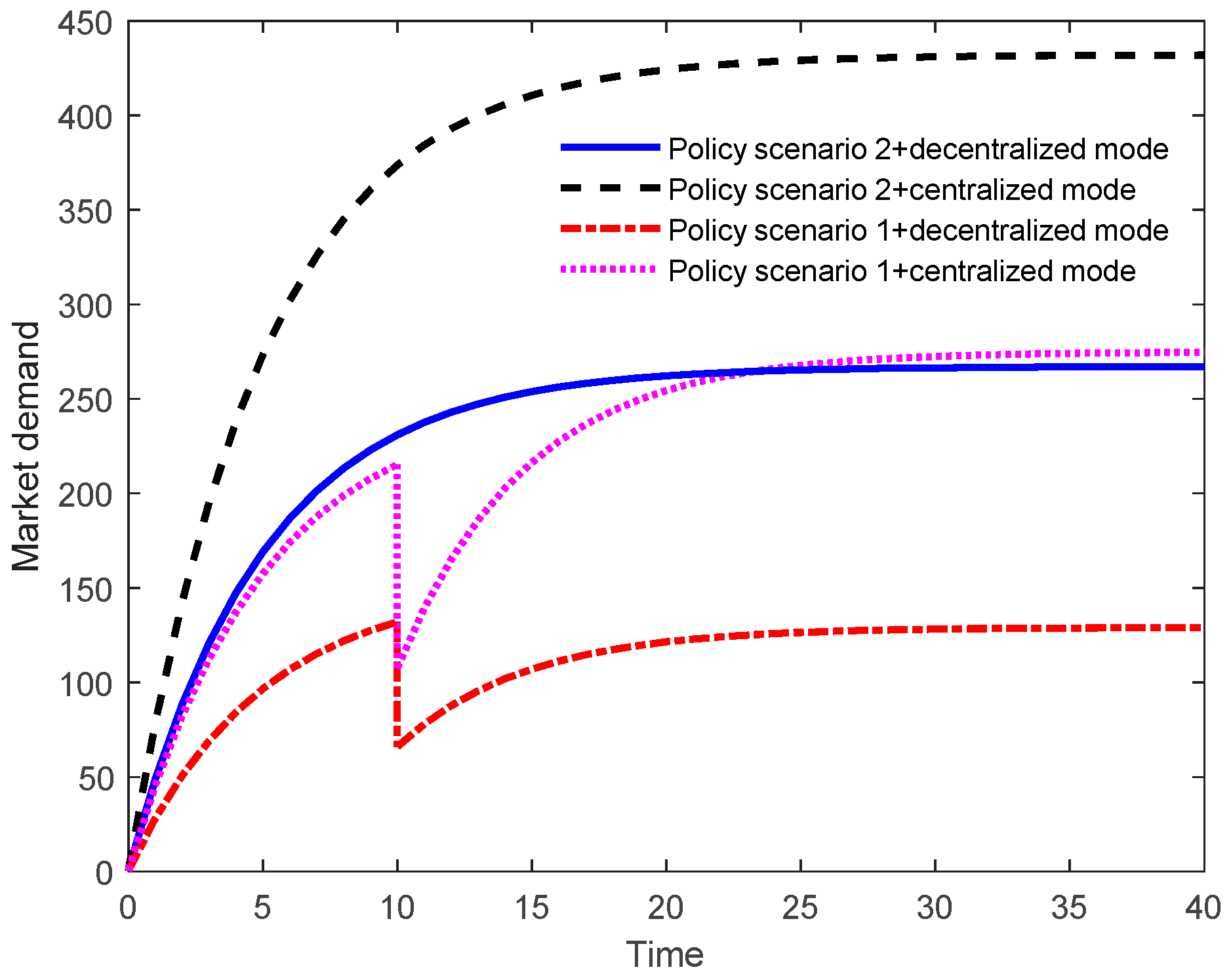
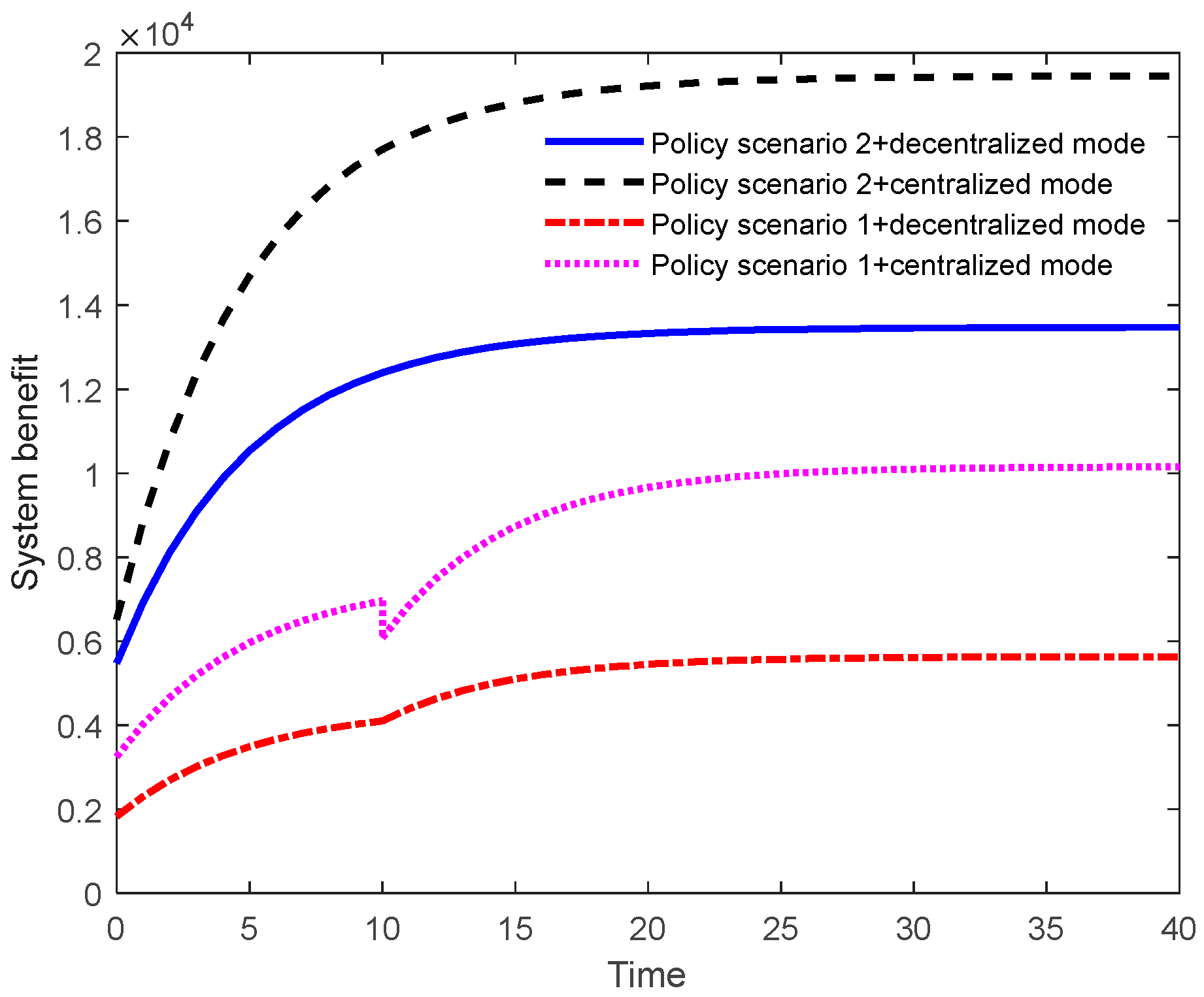
5.1. Market Demand and System Benefits

Theorems 1–4 imply that the investments of either party do not change with time. The performances of four cases (two scenarios combined with the decentralized and centralized modes) were evaluated by two other important indexes: the market demand and system benefits, which are the sum of the benefits of both parties over the entire decision-making horizon.

As shown in Figure 3, the market demand in both modes for Scenario 2 continuously grows until it stabilizes, and the centralized mode can promote the market demand to a higher level. However, in Scenario 1, a sudden drop appears in both curves due to the subsidy cancellation at this time, and the change in market demand in the centralized mode is more noticeable than in the decentralized mode. Thus, both parties should develop more conservative strategies, such as reducing investments properly in the first stage in order to mitigate the shock on the market demand, for more benefits over both stages. After the subsidy cancellation, both parties should increase their investments so that the market demand can recover to the previous level. However, it would only be able to reach a level lower than that in Scenario 2.

Figure 4 shows the system benefits in the four cases, in all of which the benefits eventually reach stable levels. Similarly to the market demand curves, both curves of the system benefits also experience perceptible changes in Scenario 1. Shortly after the cancellation in Scenario 1, the market demand and system benefits would suffer small drops, but increases in the investments by both parties would help the market demand and the marginal benefits of both to rebound, so that the system benefits would increase and eventually reach a stable level. Figure 4 also shows that the system benefits in the centralized mode are much higher whether the subsidy is canceled or not.

5.2. Parameter Sensitivity Analysis

Since the centralized game mode presents a significant advantage over the decentralized mode, we used the former as an example to explore the influences of the model’s parameters on the results.

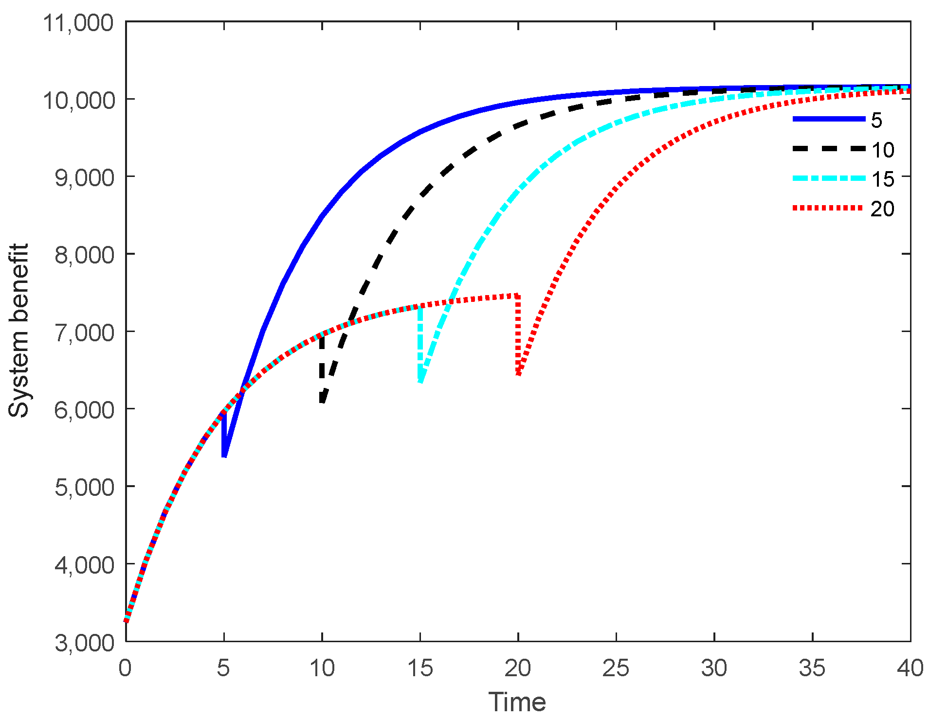
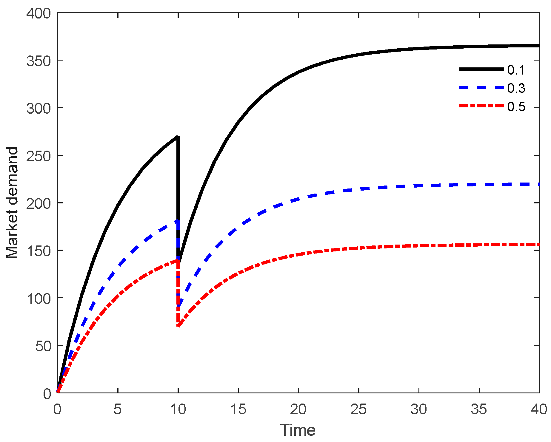
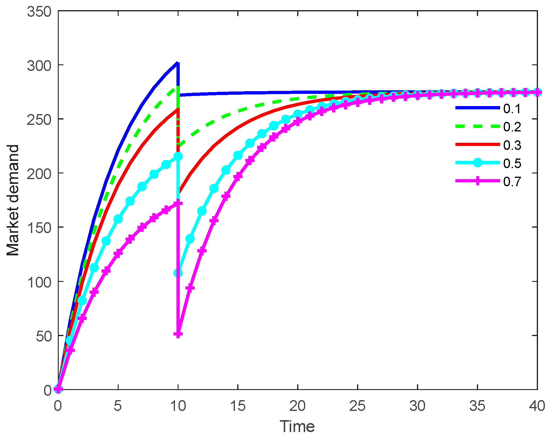
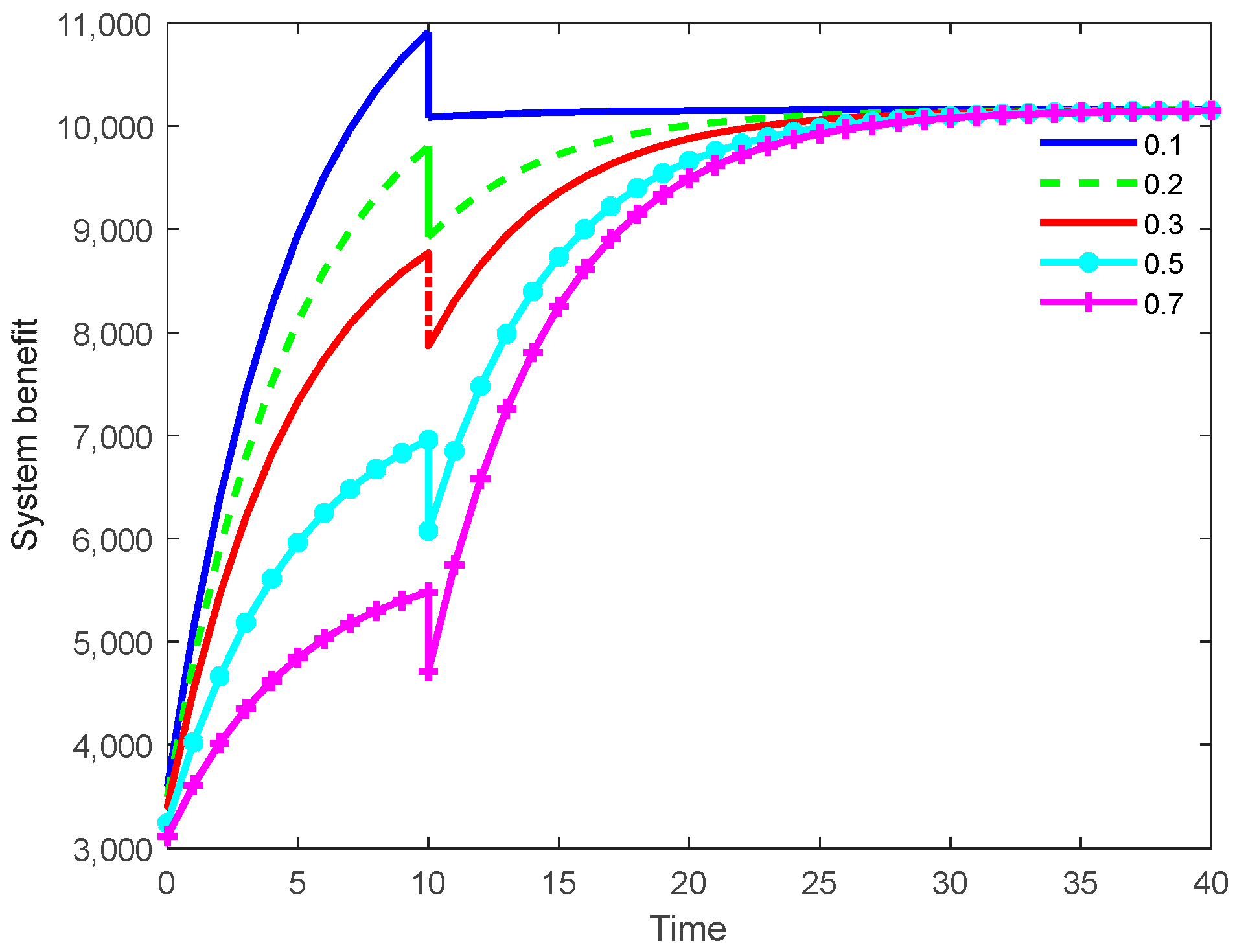
5.2.1. Effects on Market Demand and System Benefits

Figure 5 and Figure 6 show the effects on the market demand and system benefits in Scenario 1 when the subsidy cancellation occurs, at $T$ = 5, 10, 15, and 20. The jump emerges in these indexes. The effects appear shortly after each occurrence and linger until the indexes stabilize. The earlier the cancellation, the less market demand is lost. After the subsidy cancellation, both parties will change their investment levels and the market demand will gradually rise to a stable level. Moreover, the earlier the cancellation, the sooner a stable level is reached. Regardless of when the cancellation occurs, the trajectories of the market demand and system benefits are similar, indicating that the timing of the cancellation would not affect the investment levels in each stage.

Figure 7 and Figure 8 show the effects of three discount rates ($\rho$ = 0.1, 0.3, and 0.5) in Scenario 1. At a higher discount rate, the stable values of the market demand and system benefits slightly exceed the highest values in the previous stage, but greatly exceed at a lower discount rate. Therefore, each party should devise a long-term strategy, rather than focus on short-term benefits, in order to obtain higher market demand and more system benefits.

Figure 9 and Figure 10 show the effects of five rates ($\psi$ = 0.1, 0.2, 0.3, 0.5, and 0.7) of loss of market demand in Scenario 1. Different rates can still yield the same stable level for both the market demand and system benefits. When the rate for the market demand is low, both parties should increase their investments in order to boost the market demand. In the second stage, they should adjust their investments appropriately in order to stabilize it. However, the level in the second stage would not reach that in the first stage. When the rate is high, the subsidy cancellation would weaken the effectiveness of the investments in the first stage. Therefore, both parties should reduce their investments in order to keep the market demand at a lower level, which would be conducive to reducing their losses of benefits. In the second stage, both parties should increase their investments in order to push up the market demand. The changes in the system benefits are similar to those in the market demand.

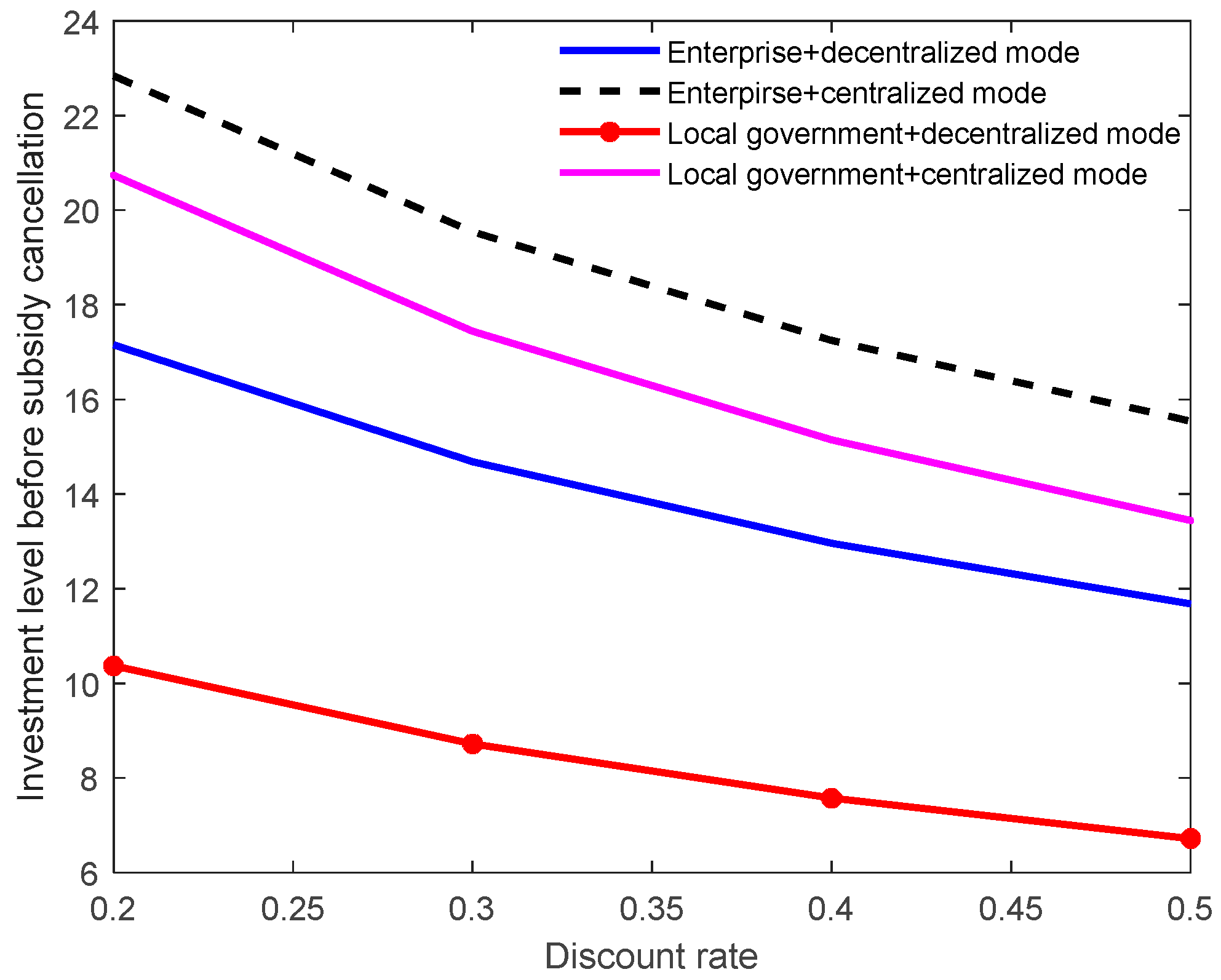
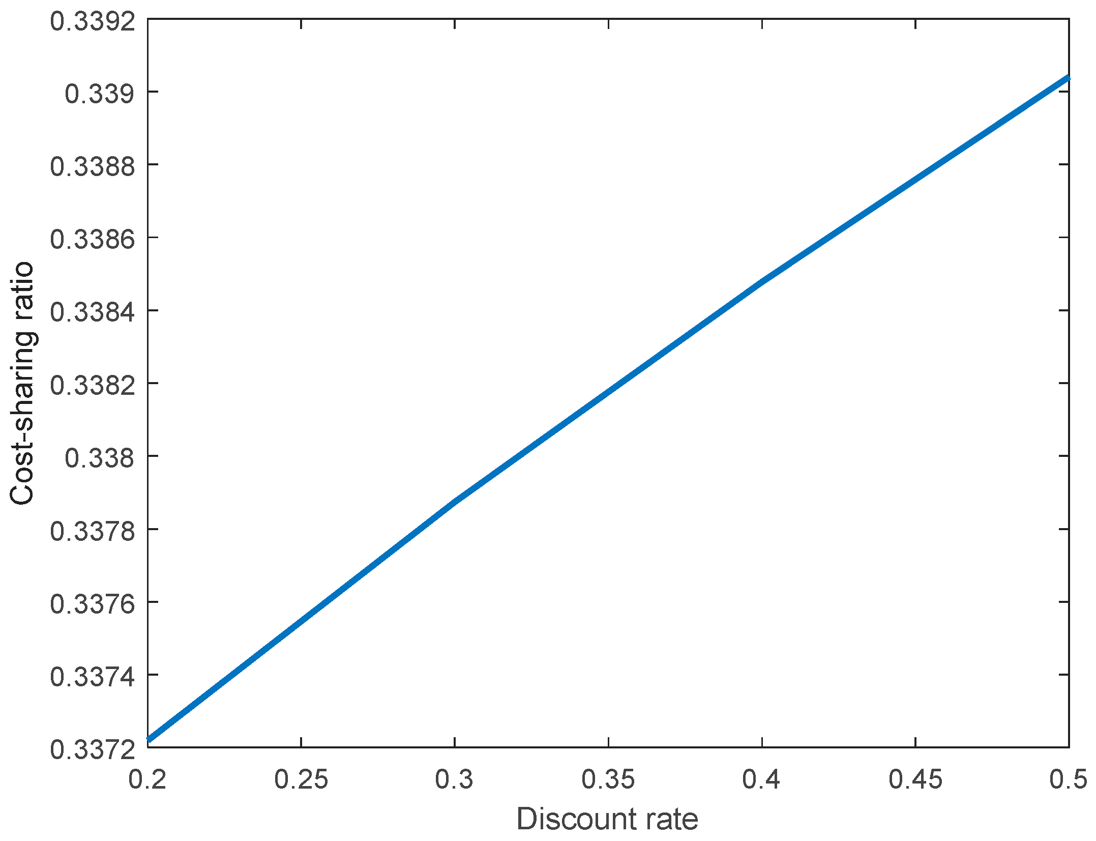
5.2.2. Effects on Optimal Strategies

The results in Section 3 demonstrate that in both modes, the discount rate has similar influences on the optimal strategies and investments of both parties, as well as on the government’s cost-sharing ratio. In addition, the changes in the rates of loss of market demand affect the investments of both parties, as well as the government’s cost-sharing ratio, in the first stage in Scenario 1. Therefore, we took this stage as an example for exploring the influences of different parameter settings on the optimal strategies of both players.

The discount rate $\rho$ varies within [0.2 0.5], while the other parameters remain unchanged. The corresponding investment levels and cost-sharing ratio in the first stage are shown in Figure 11 and Figure 12, respectively. As the discount rate increases, the investments decrease but the cost-sharing ratio grows almost linearly. In the centralized game mode, the investments of both parties are higher than in the decentralized game mode. The investment of the enterprise is higher than that of the local government, because the enterprise’s investment can not only yield fuel consumption dual-point benefits, but also generate social and environmental benefits. When the discount rate increases, both parties pay more attention to their current benefits and tend to reduce their investments in the first stage, thereby reducing the loss caused by the subsidy cancellation, but gaining more benefits over both stages.

The loss rate of the market demand is determined by many factors, such as the market environment and consumer preferences. With the loss rate varying from 0 to 1, the investments of both parties and the cost-sharing ratio in the first stage are shown in Figure 13 and Figure 14. As the loss rate of the market demand grows, the investments decrease linearly, but the cost-sharing ratio is a parabolic upward curve. The investment levels of both parties in the centralized game mode are higher. The investment level of the enterprise is higher than that of the government for the same reason in Figure 11. It is implied in Figure 14 that when the loss rate is high, the accumulated market demand in the first stage will be greatly reduced, so both parties should lower their investments at this stage in order to reduce their own losses and increase their benefits over both stages.

6. Conclusions

In this paper, a differential game between the local government and NEV enterprises was explored with regard to an NEV subsidy cancellation. The optimal investment strategies, market demand, and system benefits in the decentralized and centralized game modes of two policy scenarios are discussed. A numerical simulation was conducted and the sensitivity of the model parameters was also analyzed. The main conclusions of this paper are as follows:

(1)

In anticipation of the subsidy cancellation, both parties should formulate investment strategies for the stages before and after the cancellation, rather than for an infinite time horizon. In both modes, the investments, market demand, and system benefits are lower than they were before the cancellation. In order to face the fluctuations in market demand that would be caused by the cancellation, both parties should appropriately reduce their investments beforehand, then increase them afterward in order to maximize their benefits over both stages and promote the market demand, which could rebound due to the growing investments in the second stage. However, the market demand would be lower than it was before the cancellation.

(2)

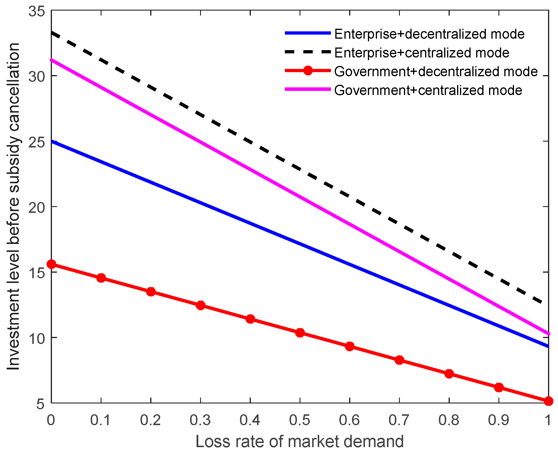
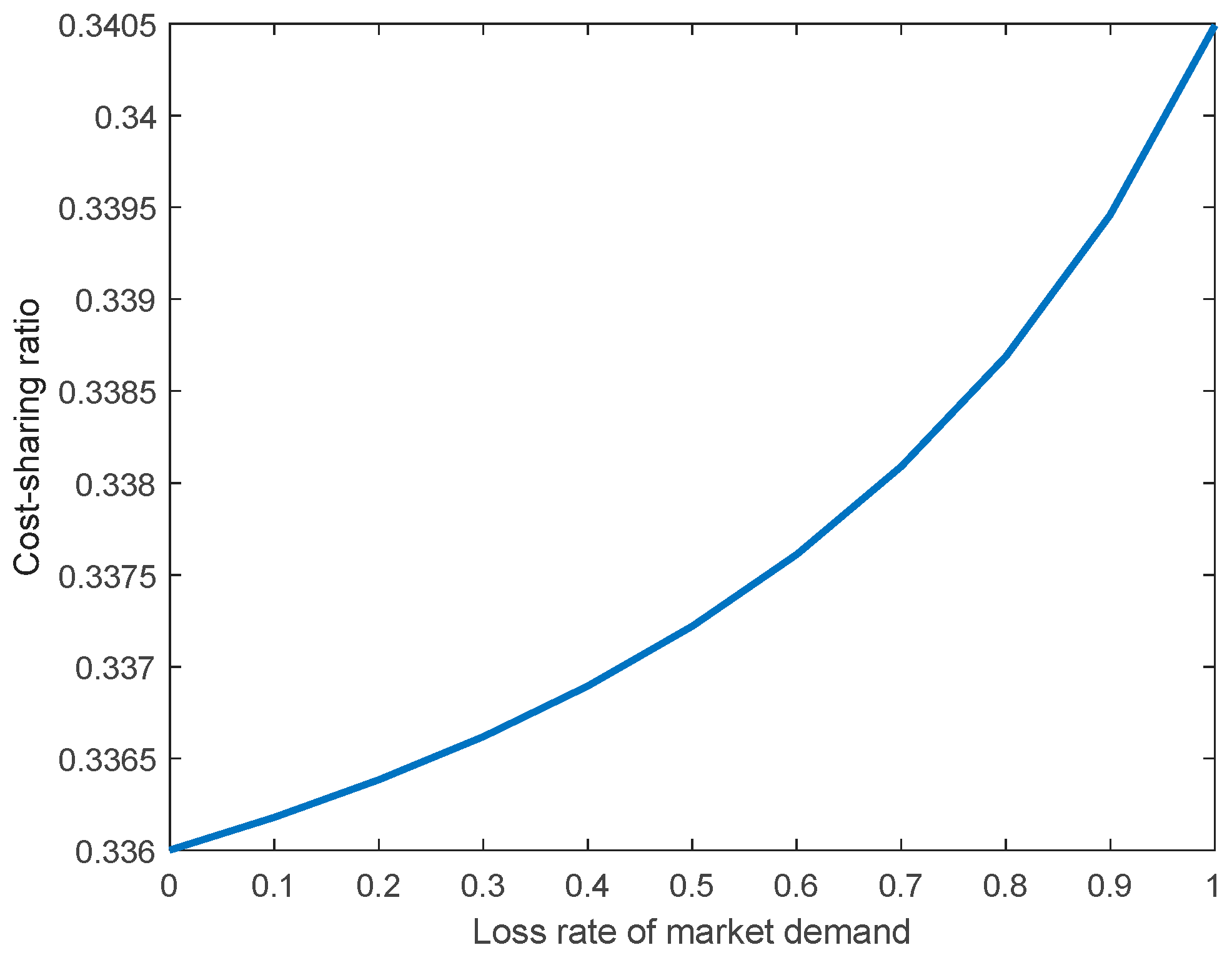
The parameter sensitivity analysis implied that the occurrences of the subsidy cancellation would not affect the investment levels of either party before and after the cancellation, but would affect the loss of market demand and system benefits at about the time of the cancellation, as well as until the market demand and system benefits stabilize. The earlier the cancellation occurs, the sooner the market demand and system benefits could stabilize so that fewer benefits would be lost. The results also showed that higher discount rates lowered the market demand and system benefits. The loss rate of the market demand does not affect its level or the system benefits. As the discount rate increases, the investments of both parties nonlinearly diminish in the first stage, but the government’s cost-sharing ratio rises linearly. With the increasing loss rate of the market demand, the investment levels of both parties show linear downward trends, whereas the government’s cost-sharing ratio is a nonlinear upward parabolic curve.

(3)

A comparison of the results of both scenarios showed that whether the subsidy was canceled or not, the optimal investments, market demand, and benefits of both the local government and enterprises in the centralized game mode were superior to those in the decentralized game mode. Hence, the centralized mode can improve the investment levels and market demand of both parties while increasing the system’s benefits and achieving Pareto optimality.

It is worth noting that the differential game model in this paper considers only the interactive relationships between the local government and enterprises. However, real-world investment strategies implemented by the local governments and NEV enterprises are influenced by many factors, such as consumers and NEV component manufacturers, which also affect production plans and product prices. The differential game model in this paper neglects such factors. Hence, future research could examine differential games among more than two parties. Moreover, future research could compare differential and evolutionary games.

References

1. Hao, H.; Ou, X.; Du, J.; Wang, H.; Ouyang, M. China’s Electric Vehicle Subsidy Scheme: Rationale and Impacts. Energy Policy 2014, 73, 722–732. [Google Scholar] [CrossRef]
2. Zhang, X.; Liang, Y.; Yu, E.; Rao, R.; Xie, J. Review of Electric Vehicle Policies in China: Content summary and Effect Analysis. Renew. Sustain. Energy Rev. 2017, 70, 698–714. [Google Scholar] [CrossRef]
3. Sheldon, T.L.; Dua, R. Effectiveness of China’s plug-in electric vehicle subsidy. Energy Econ. 2020, 88, 104773. [Google Scholar] [CrossRef]
4. Available online: https://mp.weixin.qq.com/s/vXmIU_xExiGnKwNzmI_zAQ (accessed on 13 January 2022).
5. Liu, Z.; Deng, Z.; He, G.; Wang, H.; Zhang, X.; Lin, J.; Qi, Y.; Liang, X. Challenges and Opportunities for Carbon Neutrality in China. Nat. Rev. Earth Environ. 2022, 3, 141–155. [Google Scholar] [CrossRef]
6. Zhang, S.; Chen, W. Assessing the Energy Transition in China Towards Carbon Neutrality with a Probabilistic Framework. Nat. Commun. 2022, 13, 87. [Google Scholar] [CrossRef] [PubMed]
7. Measures for Parallel Management of Average Fuel Consumption and New Energy Vehicle Credits of Passenger Vehicle Enterprises; Ministry of Industry and Information Technology: Beijing, China, 2017.
8. Zhu, Q.; Wang, Y.; Tian, Y. Analysis of an Evolutionary Game between Local Governments and Manufacturing enterprises under Carbon Reduction Policies Based on System Dynamics. Oper. Res. Manag. Sci. 2014, 23, 71–82. [Google Scholar]
9. Jiang, C.; Zhang, Y.; Li, W.; Wu, C. Evolutionary Game Study between Government Subsidy and R&D Activities of New Energy Vehicle Enterprises. Oper. Res. Manag. Sci. 2020, 29, 22–28. [Google Scholar]
10. Ji, S.; Zhao, D.; Luo, R. Evolutionary Game Analysis on Local Governments and Manufacturers’ Behavioral Strategies: Impact of Phasing out Subsidies for New Energy Vehicles. Energy 2019, 189, 116064. [Google Scholar] [CrossRef]
11. Chen, W.; Hu, Z. Using Evolutionary Game Theory to Study Governments and Manufacturers’ Behavioral Strategies under Various Carbon Taxes and Subsidies. J. Clean. Prod. 2018, 201, 123–141. [Google Scholar] [CrossRef]
12. Tang, X.; Wu, J.; Feng, B.; Wei, X.; Mao, X.; Shao, W. Research on “Subsidy Defraud” of New Energy Vehicles Enterprises Based on Signal Game. Open J. Bus. Manag. 2019, 7, 1803–1814. [Google Scholar] [CrossRef]
13. Pham, H. Continuous-time Stochastic Control and Optimization with Financial Applications; Springer: Berlin/Heidelberg, Germany, 2007. [Google Scholar]
14. Rubel, O.; Naik, P.; Srinivasan, S. Optimal Advertising When Envisioning a Product-Harm Crisis. Mark. Sci. 2011, 30, 1048–1065. [Google Scholar] [CrossRef]
15. Wang, W.; Ma, D.; Hu, J. Optimal Dynamic Advertising Strategies with Presence of Probable Product-Harm Crisis. Chin. J. Manag. Sci. 2022, 30, 204–215. [Google Scholar]
16. Wang, W.; Hu, J. Dynamic Quality and Marketing Decisions with Envision of Brand Crisis in a Dual-channel Supply Chain. J. Syst. Manag. 2022, 31, 413–427. [Google Scholar]
17. Hu, J.; Liu, Y.; Ma, D. Research on Food Supply Chain Dynamic Strategy Formulation and Coordination under the Prediction of Food Safety Crisis. Chin. J. Manag. Sci. 2021. [Google Scholar] [CrossRef]
18. Mukherjee, A.; Chauhan, S.S. The Impact of Product Recall on Advertising Decisions and Firm Profit While Envisioning Crisis or Being Hazard Myopic. Eur. J. Oper. Res. 2021, 288, 953–970. [Google Scholar] [CrossRef]
19. Rubel, O. Profiting from Product-harm Crises in Competitive Markets. Eur. J. Oper. Res. 2018, 265, 219–227. [Google Scholar] [CrossRef]
20. Lu, L.; Navas, J. Advertising and Quality Improving Strategies in a Supply Chain When Facing Potential Crises. Eur. J. Oper. Res. 2020, 288, 839–851. [Google Scholar] [CrossRef]
21. Sakamoto, H. Dynamic Resource Management under the Risk of Regime Shifts. J. Environ. Econ. Manag. 2014, 68, 1–19. [Google Scholar] [CrossRef]
22. Kamien, M.I.; Schwartz, N.L. Dynamic Optimization: The Calculus of Variations and Optimal Control in Economics & Management; North Holland, Inc.: Amsterdam, The Netherlands, 1998. [Google Scholar]
23. Bertsekas, D.P. Dynamic Programming and Optimal Control, 4th ed.; Athena Scientific: Massachusetts, MA, USA, 2017. [Google Scholar]
Figure 1. Propositions of differential game model.
Sustainability 14 12324 g001
Figure 2. Theorems and deductions of the differential game model.
Sustainability 14 12324 g002
Figure 3. Market demand in time for four combinations of scenarios and game modes.
Sustainability 14 12324 g003
Figure 4. System benefits in time for four combinations of scenarios and game modes.
Sustainability 14 12324 g004
Figure 5. Market demand in time at four occurrences of subsidy cancellation.
Sustainability 14 12324 g005
Figure 6. System benefits in time at four occurrences of subsidy cancellation.
Sustainability 14 12324 g006
Figure 7. Market demand in time at three discount rates.
Sustainability 14 12324 g007
Figure 8. System benefits in time at three discount rates.
Sustainability 14 12324 g008
Figure 9. Market demand in time at five rates of loss.
Sustainability 14 12324 g009
Figure 10. System benefits in time at five rates of loss.
Sustainability 14 12324 g010
Figure 11. Investment levels of both parties at discount rates before the subsidy cancellation for both game modes.
Sustainability 14 12324 g011
Figure 12. Local government’s cost-sharing ratio at discount rates before the subsidy cancellation.
Sustainability 14 12324 g012
Figure 13. Investment levels of both parties at loss rates of market demand in different game modes before the subsidy cancellation.
Sustainability 14 12324 g013
Figure 14. Local government’s cost-sharing ratio at loss rates of market demand.
Sustainability 14 12324 g014