Wave Analysis of Thick Rectangular Graphene Sheets: Thickness and Small-Scale Effects on Natural and Bifurcation Frequencies

Abstract

Free vibration and wave analysis of thick rectangular graphene are studied by employing the wave propagation method. To consider small-scale effects and thickness of a plate in nanoscales, equations of motions are represented by the Eringen nonlocal theory coupled with the Mindlin plate theory of thick plates. To solve the governing equations of motion with the wave propagation technique, propagation and reflection matrices are derived. These matrices are combined to obtain exact natural frequencies of graphene sheets for all six possible boundary conditions. To check the accuracy and reliability of the method, natural frequencies are compared with the results of the literature, and excellent agreement is observed. Additionally, wave analysis of the graphene sheet is performed and different types of waves in the graphene sheet are captured. Deriving the dispersion relation of the graphene sheet, bifurcation frequencies (cut-off and escape frequencies) are analytically found. Finally, the effects of graphene sheet thickness and nonlocal parameter on the natural frequencies and bifurcation frequencies are investigated. It is observed that natural frequencies are highly dependent on the graphene sheet’s thickness and nonlocal parameter. More importantly, the number and order of bifurcation frequencies depend on these two parameters as well. Our findings are valuable for the sustainable design and fabrication of graphene-based sensors, in which structural health monitoring of embedded graphene sheets is of great importance.

1. Introduction

Nanotechnology is a branch of technology that deals with nanoscale materials and structures. Nanomaterials have been the subject of much research in recent years, and this is motivated by their superior mechanical properties and new applications in nanoscience, nanomanufacturing, and smart nanostructure technologies. There are different nanostructures among which graphene sheets have been of high interest to researchers due to a wide range of applications [1,2,3,4,5,6]. However, there are always complications in the design, manufacturing, and health monitoring of such structures on this scale. Considering these structures as waveguides can significantly facilitate the analysis of such structures. The wave propagation method formulates the waveguide hypothesis of a medium and is a powerful tool to analyze a structure.

There are many applications associated with graphene ranging from structural health monitoring to medicine and biology. Structural health monitoring (SHM) and sensor technologies play a vital role in monitoring the condition of structures and identifying damage that may have occurred while in service.

Conventional, rigid, bulky, and discrete sensors may not be suitable for embedment, and there is a pressing need to develop flexible, robust, wireless, and thin filmlike sensors that can be easily embedded in structures. The majority of flexible strain sensors are based on graphene sheets and nanoplates as sensing elements [7,8,9,10,11].

Graphene, owing to its extraordinary multiple properties, such as ultrahigh carrier mobility, excellent electrical conductivity, superior thermal conductivity, large theoretical specific surface area, high optical transmittance, high Young’s modulus, and outstanding mechanical flexibility [12], is a promising 2D material in many applications, especially for the development of wearable sensors and implantable devices in health monitoring.

Graphene-based sensors used for human health monitoring have been reported, including wearable sensors, as well as implantable devices, which can measure body temperature, respiration rate, and electromyogram signals in real-time [13,14,15,16,17].

In these applications, the wave properties of graphene sheets are an important parameter for structural health monitoring of the embedded graphene.

In nanoscales, due to the significant effects of long-range interatomic and intermolecular electrostatic forces on mechanical behavior (called small-scale effects), classical continuum mechanics theories are insufficient for analyzing their static and dynamic behavior. Methods are developed to consider small-scale effects in analyzing different systems on nano or micro scales.

The molecular dynamics simulation methods [18] is a type of N-body simulation by which one can study the physical movements of atoms and molecules. Although a large number of studies have employed this method for micro and nanoscale analysis [19,20,21,22,23,24,25], it is not time-efficient, especially when the number and range of atoms increase. Eringen [26] introduced nonlocal elasticity theory that encompasses both features of lattice parameters and classical elasticity. Many studies have employed this well-known theory that formulates small-length scale effects by considering a material length scale as a parameter in its constitutive equations. Peddieson et al. [27] proposed the formulation of a nonlocal version of the Euler–Bernoulli beam by applying nonlocal elasticity and showed that this theory is a potential remedy for the analysis of nanostructures. Hence, axial vibration of nanorods and single-walled carbon nanotubes [28], a first-known dynamic stability analysis of carbon nanotube-reinforced functionally graded (CNTR-FG) cylindrical panels under static and periodic axial force [29], and the vibration behavior of quadrilateral single-layered graphene sheets (SLGSs) in a magnetic field using classic plate theory and incorporating nonlocal elasticity theory [30] are solved by employing this theory. Additionally, the dynamic and buckling behavior of graphene sheets are the focus of some literature. Pradhan and Phadikar [31] integrated the nonlocal theory into classical plate theory (CLPT) and first-order shear deformation theory (FSDT) of plates and solved the governing equations for simply supported boundary conditions using Navier’s approach. Later on, in another study [32], they employed the finite element method to analyze nanoplate vibrations. Aghababaei and Reddy [33] reformulated the third-order shear deformation theory of Reddy using the nonlocal linear elasticity theory of Eringen and presented analytical solutions for bending and free vibration of a simply supported rectangular plate. Asbaghian Namin and Pilafkan [34], using the generalized differential quadrature method (GDQ), solved the free vibration of defective graphene sheets via nonlocal elasticity theory. Hosseini Hashemi et al. [35] investigated Mindlin rectangular nanoplate vibrations using an exact analytical approach. However, they did not report thickness effects on natural and bifurcation frequencies, and there is no wave analysis in their study.

Even though there are some studies for analytical and exact solutions of the nonlocal plate theory [35,36,37,38], they apply boundary conditions to the general solution of the differential equation to obtain the natural frequencies. The wave propagation method is an alternative approach which considers vibrations as propagating waves traveling in a medium called waveguide. In this method, the solution is presented in matrix form that benefits programming purposes [39,40]. A wide range of researchers employed this method for their analysis. However, the majority of researchers used this method as a semi-analytical, not an exact method, or for macroscale analysis. Mace [41] studied the free vibrations of the Euler–Bernoulli beam and the Timoshenko beam by considering the wave propagation approach, and Tan [42] presented wave motions in an axially strained and rotating Timoshenko shaft. Furthermore, Lee et al. [43] analyzed the non-uniform waveguides such as non-uniform bars and non-uniform Euler–Bernoulli beams whose properties vary rapidly but deterministically. Mei et al. [44] considered the wave method for free and forced vibrations of axially loaded cracked Timoshenko beams. The wave approach was applied by Lee et al. [43] to thin, uniform, and curved beams with constant curvature to obtain the natural frequencies of curved beams. In 2010, Mei [45] presented an exact wave-based analytical solution, which takes the coupling effect between bending and longitudinal vibration for the natural frequencies of classical planar frame structures. Moreover, a wave vibration approach was used by Mei [46] to study the effects of lumped end mass on the bending vibrations of a Timoshenko beam in 2011. More recently, Mei [47] applied the wave method to obtain the natural frequencies and mode shapes of single-story multi-bay planar frame structures. Supplementary to these, the modified wave approach was used by Bahrami et al. [48] to find the natural frequencies of non-uniform beams, using Euler-Bernoulli beam theory. Bahrami et al. [49], in another study, developed this method for free vibration of non-uniform rectangular membranes. Moreover, the nonlocal scale effect on vibration, buckling, and wave reflection in beams has also been studied [50]. In addition, the free vibration, wave power transmission, and reflection in multi-cracked nanobeams [51] and nanorods [52] were studied by Bahrami. Analysis of nanoplates using a wave propagation approach was investigated by Bahrami and Teimourian [53], and they studied the small-scale effect on vibration and wave power reflection in circular annular thin graphene sheets. Recently, Mousavi Janbeh Sarayi et al. [54,55] presented an exact analytical solution for the vibration of macroscale Mindlin plates using the exact analytical wave method. They employed the wave method to provide benchmark results for natural frequencies of thick plates and analyze the power reflection at boundaries. They found that there are three cut-off frequencies, which are essential in analyzing power reflection at boundaries, for a thick plate.

The graphene sensor usually Is printed directly on the sample and on a PET (polyethene terephthalate) transfer film on the sample. This is due to the fact that sometimes the material is conductive, and the signal would be affected by attaching the graphene sensor directly to the surface of the sample. Graphene-based sensors evaluate the strain generated within a material. The graphene sensor proved to be able to evaluate strain at various levels providing a gauge factor higher than commercially available strain gauges. Akram Zitoun et al. [56] present a strain sensing system based on graphene. The graphene is selected as the sensing material to investigate the capability of printing custom- designed sensors to monitor composite materials instead of the use of commercially available strain gauges.

According to the present literature review, there are a few papers based on the wave propagation method for vibration and wave analysis of graphene sheets.

It is also worth mentioning that some research uses nanoplates as a sensing element in sensors [9,10,11] which have a greater thickness. Since nonlocal theory considers the microscopic effect in any nanostructure, whether it is a graphene sheet or thick nanoplate, we tried to consider the effect of thickness regardless of the nature of our nanostructure.

In this regard, thin plate theory cannot accurately predict the actual behavior of such nanostructures. In addition, macroscale analysis lacks the consideration of the small-scale effects that are essential for energy analysis in nanomaterials. Therefore, the wave analysis of macro and thin plate theories cannot be applied to a thick graphene sheet, and there is only one literature about energy transmission and wave analysis in thick nanostructures, namely, for Timoshenko nanobeams [57]. A simple exact analytical solution using the wave propagation approach in thick nanoplates seems essential due to the practical usage of these structures in structural health monitoring. This approach provides the chance of finding analytical cut-offs and escape frequencies in a graphene sheet. In this study, an exact analytical solution is presented to analyze the wave motion and free vibration in thick rectangular graphene sheets using the wave approach. The natural frequencies obtained with this approach are compared with the results in other literature. Benchmark results are presented with any combination of boundary conditions for Levy-type plates, and the effect of nonlocal parameter, thickness ratio of the graphene sheet, plate’s aspect ratio, and number of half waves on natural frequencies are investigated. It is shown that these analytical results provide important information about wave propagation and energy analysis in the medium. For example, there are four cut-off and three escape frequencies, whose existence and order of appearance depend on nonlocal parameter and thickness ratio of the plate. It is shown that thickness ratio of the graphene sheet and nonlocal parameter significantly affect the combination of ongoing waves in the graphene sheet and its natural frequencies. The results and methods of this study can be applied to future work associated with graphene sheet wave analysis. Moreover, understanding how changes to physical parameters affect wave propagation through graphene materials is essential to understanding the complete behavior of sensors with the implemented graphene material. Possible sources of uncertainty and error could occur by a lack of understanding of the complete graphene behavior, and thus the utilization of our current study can be of interest to many of these researchers.

2. Materials and Methods

2.1. Governing Equations

Consider a thick graphene sheet of length a, width b, and uniform thickness h, oriented so that its undeformed middle surface contains the $x_1$ and $x_2$ axis of a Cartesian coordinate system $\left(x_1,x_2,x_3\right)$, as shown in Figure 1. Displacements along the $x_1$ and $x_2$ axes are denoted by $U_1$ and $U_2$, respectively, while displacement in the perpendicular direction to the $x_1$-$x_2$ plane is denoted by $U_3$. In the Mindlin plate theory [58], the displacement components are given as:

$$U_1\left(x_1,x_2,x_3,t\right)=u_1\left(x_1,x_2\right)+x_3{\varphi }_1\left(x_1,x_2,t\right)$$

(1a)

$$U_2\left(x_1,x_2,x_3,t\right)=u_2\left(x_1,x_2\right)+x_3{\varphi }_2\left(x_1,x_2,t\right)$$

(1b)

$$U_3\left(x_1,x_2,x_3,t\right)=u_3\left(x_1,x_2,t\right)$$

(1c)

where t is time,$U_1$ and $U_2$ are inplane displacement on the mid plane (i.e., $x_3=0$), $U_3$ is the transverse displacement, and ${\varphi }_i \left(i=1,2\right)$ are the slopes due to bending alone on the respective planes.

The equations of motion of Mindlin plate theory in nonlocal continuum model for in-plane and out-of-plate displacements are uncoupled [35], so we consider only equations of motion for flexural vibration for simplicity and, for generalizing results, in nondimensional form as follows:

$$\left[12k{\nu }_1-{\tau }^2{\beta }^2{\delta }^2\right]{\tilde{\nabla }}^2{\tilde{u}}_3 + \beta {\delta }^2{\tilde{u}}_3 + 12k{\nu }_1\left({\tilde{\varphi }}_{1,1} + {\tilde{\varphi }}_{2,2}\right)=0$$

(2a)

$$\begin{gathered} \left[{\nu }_1-\frac{{\tau }^2{\beta }^2{\delta }^2}{12}\right]{\tilde{\nabla }}^2{\tilde{\varphi }}_1 + \left[\frac{{\beta }^2{\delta }^2}{12}-\frac{12k{\nu }_1}{{\delta }^2}\right]{\tilde{\varphi }}_1 + \left(1-{\nu }_1\right)\left({\tilde{\varphi }}_{1,11} + {\tilde{\varphi }}_{2,21}\right) \\ -\frac{12k{\nu }_1}{{\delta }^2}{\tilde{u}}_{3,1}=0, \end{gathered}$$

(2b)

$$\begin{gathered} \left[{\nu }_1-\frac{{\tau }^2{\beta }^2{\delta }^2}{12}\right]{\tilde{\nabla }}^2{\tilde{\varphi }}_2 + \left[\frac{{\beta }^2{\delta }^2}{12}-\frac{12k{\nu }_1}{{\delta }^2}\right]{\tilde{\varphi }}_2 + \left(1-{\nu }_1\right)\left({\tilde{\varphi }}_{1,12} + {\tilde{\varphi }}_{2,22}\right) \\ -\frac{12k{\nu }_1}{{\delta }^2}{\tilde{u}}_{3,2}=0, \end{gathered}$$

(2c)

where the nondimensional Laplacian operator is defined as ${\tilde{\nabla }}^2=\frac{{\partial }^2}{\partial X_1^2} + \frac{{\partial }^2}{\partial X_2^2}$ and nondimensional terms are considered as below:

$$\begin{gathered} X_1=\frac{x_1}{a}, X_2=\frac{x_2}{a}, \delta =\frac{h}{a}, \eta =\frac{b}{a}, {\tilde{\varphi }}_i={\varphi }_i \left(i=1,2\right) \\ {\tilde{u}}_3=\frac{u_3}{a}, \tau =\frac{\mu }{a}, {\tilde{\mathit{\nabla }}}^2=a^2{\mathit{\nabla }}^2, \beta =\omega a^2\sqrt{\frac{\rho h}{D}} \end{gathered}$$

(3)

In these equations,$\tau$ and $\beta$ are nondimensional nonlocal and frequency parameters, respectively, $\delta$ is the thickness ratio, $\eta$ is the aspect ratio, $\mu$ is the nonlocal parameter, $\nu$ is the Poisson’s ratio, and ${\nu }_1=\left(1-\nu \right)/2$; the shear correction factor $k$ is introduced to consider that the transverse shear strains depend on the thickness coordinate $x_3$; $D=E{h}^3/12\left(1-{\nu }^2\right)$ is the flexural rigidity, and the inertia term $I_k$ is defined as:

$$I_l={{\displaystyle \int }}_{-\frac{h}{2}}^{+\frac{h}{2}}\rho x_3^{l}d{x}_3 l=0,2$$

(4)

where $\rho$ is the mass density per unit volume. Dimensionless nonlocal forces and moment resultants can be obtained in terms of dimensionless local ones as [59]:

$$\left[1-{\tau }^2{\tilde{\nabla }}^2\right]{\tilde{Q}}_{ij}={\tilde{Q}}_{ij}^L, \left[1-{\tau }^2{\tilde{\nabla }}^2\right]{\tilde{M}}_{ij}={\tilde{M}}_{ij}^L,$$

(5)

where ${\tilde{Q}}_{ij}$ and ${\tilde{M}}_{ij}$ are nonlocal force and moment resultants and ${\tilde{Q}}_{ij}^L$ and ${\tilde{M}}_{ij}^L$ are local force and moment resultant. Local force and moment resultants are:

$${\tilde{M}}_{11}^L=-\left({\tilde{\varphi }}_{1,1} + \nu {\tilde{\varphi }}_{2,2}\right)e^{i\omega t},$$

(6a)

$${\tilde{M}}_{22}^L=-\left({\tilde{\varphi }}_{2,2} + \nu {\tilde{\varphi }}_{1,1}\right)e^{iwt},$$

(6b)

$${\tilde{M}}_{12}^L={\tilde{M}}_{21}=-{\nu }_1\left({\tilde{\varphi }}_{2,2} + {\tilde{\varphi }}_{1,1}\right)e^{iwt},$$

(6c)

$${\tilde{N}}_{13}^L=-\left({\tilde{\varphi }}_1-{\tilde{u}}_{3,1}\right)e^{i\omega t},$$

(6d)

$${\tilde{N}}_{23}^L=-\left({\tilde{\varphi }}_2-{\tilde{u}}_{3,2}\right)e^{i\omega t},$$

(6e)

Three types of nondimensional, nonlocal boundary conditions along $x_2$ axes (i.e., $X_2=0$ or $X_2=\eta$) are as follows:

$$\begin{array}{ll}{\tilde{M}}_{22}=0, {\tilde{\varphi }}_1=0, {\tilde{u}}_3=0,& \mathrm{Simply}\mathrm{supported}\mathrm{edge}\left(\mathrm{S}\right),\end{array}$$

(7a)

$$\begin{array}{ll}{\tilde{\varphi }}_1=0, {\tilde{\varphi }}_2=0, {\tilde{u}}_3=0,& \mathrm{Clamped}\mathrm{edge}\left(\mathrm{C}\right),\end{array}$$

(7b)

$$\begin{array}{ll}{\tilde{M}}_{22}=0, {\tilde{M}}_{21}=0, {\tilde{N}}_{23}=0,& \mathrm{Free}\mathrm{edge}\left(\mathrm{F}\right).\end{array}$$

(7c)

Considering Equations (5) and (7), it can be found that the local boundary conditions and nonlocal ones can be used interchangeably for the present boundary conditions.

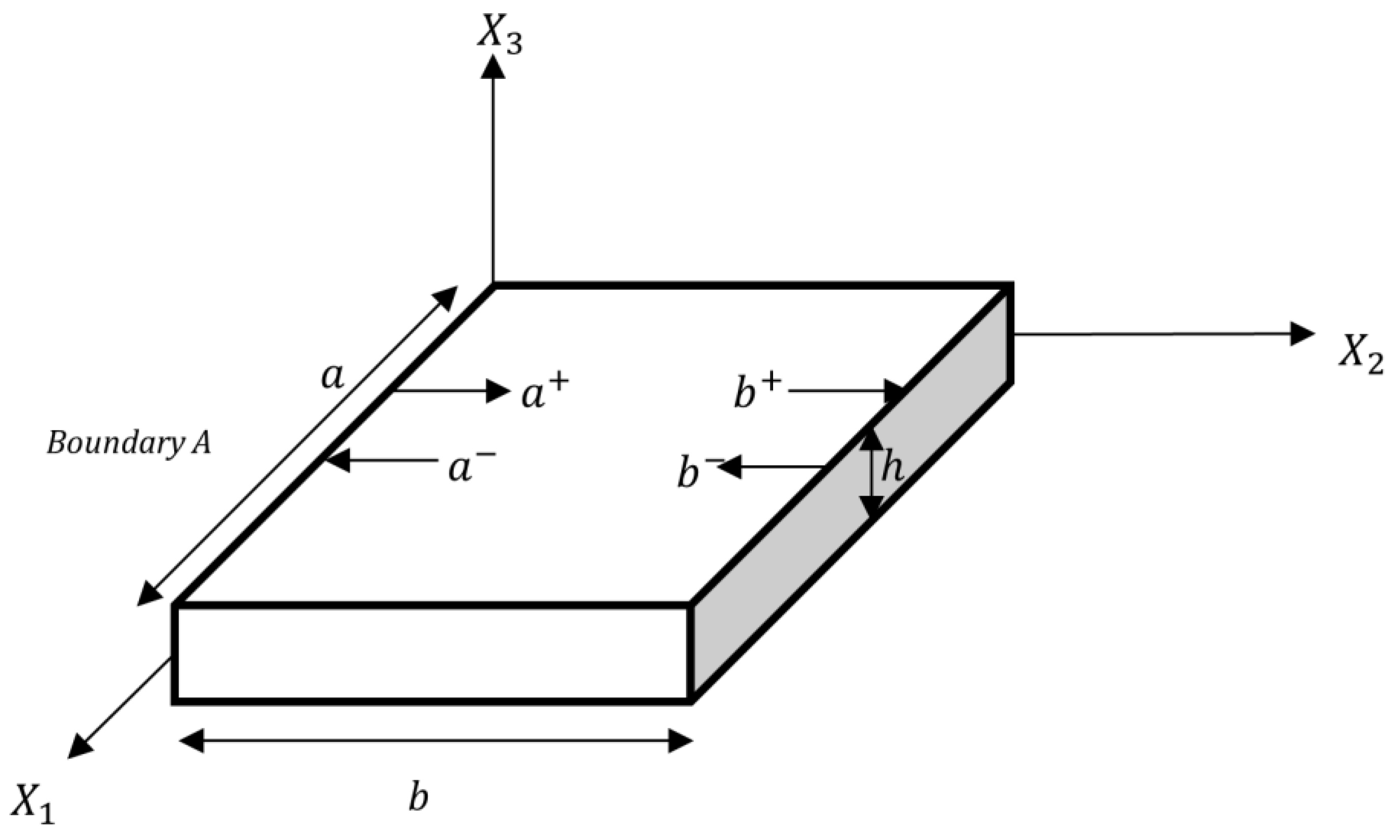
2.2. Exact Wave Solution Procedure

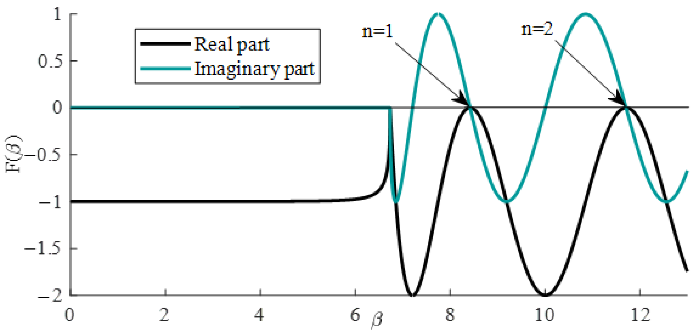
Assume harmonic motion with respect to time as

$${\tilde{\varphi }}_i\left(X_1,X_2,t\right)={\tilde{\varphi }}_i\left(X_1,X_2\right)e^{i\omega t} \left(i=1,2\right), {\tilde{u}}_3\left(X_1,X_2,t\right)={\tilde{u}}_3\left(X_1,X_2\right)e^{i\omega t},$$

(8)

and potential functions, $W_1, W_2,$ and $W_3$, for representing equations of motion’s variables as [35]:

$${\tilde{\varphi }}_1=C_1{W}_{1,1} + C_2{W}_{2,1} + W_{3,2}$$

(9a)

$${\tilde{\varphi }}_2=C_1{W}_{1,2} + C_2{W}_{2,2}-W_{3,1}$$

(9b)

$${\tilde{u}}_3=W_1 + W_2$$

(9c)

By substituting these equations into Equation (2), the uncoupled equations of motion are derived as:

$${\tilde{\nabla }}^2{W}_r + {\alpha }_r{W}_r=0, r=1, 2, 3$$

(10)

where in Equations (9) and (10)

$$\begin{gathered} C_i=\frac{d_i}{{\alpha }_i^2\left(\frac{{\tau }^2{\beta }^2{\delta }^2}{12}-{\nu }_1\right) + \frac{{\beta }^2{\delta }^2}{12}-\frac{12k_s{\nu }_1}{{\delta }^2}}, \left(i=1,2\right) \\ {d}_i=\frac{12k_s{\nu }_1}{{\delta }^2}-\left(1-{\nu }_1\right)b_i, b_i=\frac{{\alpha }_i^2\left(12k_s^2{\nu }_1-{\tau }^2{\beta }^2{\delta }^2\right)-{\beta }^2{\delta }^2}{12k_s^2{\nu }_1}, \left(i=1,2\right) \end{gathered}$$

(11)

and

$$\begin{gathered} {\alpha }_1^2=\frac{a_2-\sqrt{\left(a_2^2-4a_1{a}_3\right)}}{2a_1}, {\alpha }_2^2=\frac{a_2 + \sqrt{\left(a_2^2-4a_1{a}_3\right)}}{2a_1}, {\alpha }_3^2=\frac{\frac{{\beta }^2{\delta }^2}{12}-\frac{12k_s^2{\nu }_1}{{\delta }^2}}{{\nu }_1-\frac{{\tau }^2{\beta }^2{\delta }^2}{12}}, \\ {a}_1=\left(-1 + \frac{{\tau }^2{\beta }^2{\delta }^2}{12}\right) + \frac{\left(1-\frac{{\tau }^2{\beta }^2{\delta }^2}{12}\right){\tau }^2{\beta }^2{\delta }^2}{12k_s^2{\nu }_1}, \\ {a}_2=\frac{\left(-6 + {\tau }^2{\beta }^2{\delta }^2\right){\beta }^2{\delta }^4-6k_s^2\left(12{\tau }^2{\beta }^2{\delta }^2 + {\beta }^2{\delta }^4\right){\nu }_1}{72k_s^2{\delta }^2{\nu }_1}, \\ {a}_3=\frac{{\beta }^2{\delta }^2\left(\frac{12k_s^2{\nu }_1}{{\delta }^2}-\frac{{\beta }^2{\delta }^2}{12}\right)}{12k_s^2{\nu }_1} \end{gathered}$$

(12)

Considering simply supported edges at $X_1=0$ and $X_1=1$ and Equations (9) and (10), the Levy type solution of Equation (2) is found as:

$$\begin{gathered} {\tilde{\varphi }}_1=\left[A_1{C}_{1}m\pi e^{i{\lambda }_1{X}_2} + A_2{C}_{1}m\pi e^{-i{\lambda }_1{X}_2} + A_3{C}_{2}m\pi e^{{\lambda }_2{X}_2} + A_4{C}_{2}m\pi e^{-{\lambda }_2{X}_2} \\ + A_5{\lambda }_3\eta e^{{\lambda }_3{X}_2} + A_6{\lambda }_3\eta e^{-{\lambda }_3{X}_2}\right]\cos \left(m\pi X_1\right) \end{gathered}$$

(13a)

$$\begin{gathered} {\tilde{\varphi }}_2=\left[A_{1}i{C}_1{\lambda }_1\eta e^{i{\lambda }_1{X}_2}-A_{2}i{C}_1{\lambda }_1\eta e^{-i{\lambda }_1{X}_2} + A_3{C}_2{\lambda }_2\eta e^{{\lambda }_2{X}_2}-A_4{C}_2{\lambda }_2\eta e^{-{\lambda }_2{X}_2} + A_{5}m\pi e^{{\lambda }_3{X}_2} \\ -A_{6}m\pi e^{-{\lambda }_3{X}_2}\right]\sin \left(m\pi X_1\right) \end{gathered}$$

(13b)

$${\tilde{u}}_3=\left[A_1{e}^{i{\lambda }_1{X}_2} + A_2{e}^{-i{\lambda }_1{X}_2} + A_3{e}^{{\lambda }_2{X}_2} + A_4{e}^{-{\lambda }_2{X}_2}\right]\sin \left(m\pi X_1\right)$$

(13c)

where ${\lambda }_i \left(i=1, 2, 3\right)$ are wavenumbers. A transformation from the physical domain into the wave domain can be made (as explained in detail in the next section) and the dispersion relation for each wave component is obtained as follows:

$${\lambda }_1^2={\alpha }_1^2-{\left(m\pi \right)}^2, {\lambda }_2^2={\alpha }_2^2 + {\left(m\pi \right)}^2, {\lambda }_3^2={\alpha }_3^2 + {\left(m\pi \right)}^2$$

(14)

Based on these equations, the type of waves in the graphene sheets is defined. There are mainly three types of oscillating waves in a medium: propagating, evanescent, and decaying waves. Qualitative behavior of wavenumbers, meaning that whether a wavenumber is a real, imaginary, or complex number, defines the type of wave.

2.3. Wave Analysis

From a wave motion standpoint, vibrations propagate in any object and reflect at boundaries. We describe them in matrix form, the so-called propagation and reflection matrices. The positive- and negative-going wave solutions of Equation (13) can be defined as:

$$a^{+}=\left\{\begin{array}{c}{A}_2{e}^{-i{\lambda }_1{X}_2}\\ A_4{e}^{-{\lambda }_2{X}_2}\\ A_6{e}^{-{\lambda }_3{X}_2}\end{array}\right\}, a^{-}=\left\{\begin{array}{c}{A}_1{e}^{i{\lambda }_1{X}_2}\\ A_3{e}^{{\lambda }_2{X}_2}\\ A_5{e}^{{\lambda }_3{X}_2}\end{array}\right\}.$$

(15)

Consider two points on a flexural vibrating plate along the $X_2$-direction at a distance $b/a$ apart. The positive- and negative-going wave vectors at these points are denoted as $a^{+}, a^{-}, b^{+},$ and $b^{-}$ respectively as shown in Figure 1. These wave vectors are related together by the following relation written in wave format:

$$\begin{gathered} b^{+}=f^{+}\left(b\right)a^{+} \\ {a}^{-}=f^{-}\left(b\right)b^{-}, \end{gathered}$$

(16)

where $f^{+}\left(x\right)$ is known as the propagation matrix in the positive direction ($+X_2$), and $f^{-}\left(x\right)$ is known as the propagation matrix in the negative direction ($-X_2$). From Equation (15), waves at $X_2=0$ and $X_2=\eta$ are obtained as:

$$a^{+}=\left\{\begin{array}{c}{A}_2{e}^{-i{\lambda }_{1}0}\\ A_4{e}^{-{\lambda }_{2}0}\\ A_6{e}^{-{\lambda }_{3}0}\end{array}\right\}, a^{-}=\left\{\begin{array}{c}{A}_1{e}^{i{\lambda }_{1}0}\\ A_3{e}^{{\lambda }_{2}0}\\ A_5{e}^{{\lambda }_{3}0}\end{array}\right\},b^{+}=\left\{\begin{array}{c}{A}_2{e}^{-i{\lambda }_{1}b/a}\\ A_4{e}^{-{\lambda }_{2}b/a}\\ A_6{e}^{-{\lambda }_{3}b/a}\end{array}\right\}, b^{-}=\left\{\begin{array}{c}{A}_1{e}^{i{\lambda }_{1}b/a}\\ A_3{e}^{{\lambda }_{2}b/a}\\ A_5{e}^{{\lambda }_{3}b/a}\end{array}\right\}.$$

(17)

Considering expressions (16) and (17), the following propagation matrix for a graphene sheet is found as:

$$f^{+}\left(b\right)=f^{-}\left(b\right)=\left[\begin{array}{ccc}{e}^{-i{\lambda }_{1}b/a}& 0& 0\\ 0& e^{-{\lambda }_{2}b/a}& 0\\ 0& 0& e^{-{\lambda }_{3}b/a}\end{array}\right]$$

(18)

The reflection matrices depend on the type of boundary conditions. Thus, the reflection matrices should be calculated separately for each boundary condition. Generally, each wave as $a^{+}$ gives rise to a reflected wave as $a^{-}$, which are related by a matrix as $r$, just like below:

$$a^{+}=r{a}^{-}$$

(19)

Three types of boundary conditions are considered here: simply supported, clamped, and free boundary conditions. However, based on the fact that local boundary conditions can be employed in place of nonlocal ones, as shown in Section 2 of the present study, using waves of Equation (15) and boundary conditions of Equation (7), the reflection matrices for a Mindlin nanosheet are found as below:

Simply supported boundary at $X_2=0,\eta$:

$$r_s=r_s^L=-I_{3\times 3}$$

(20)

Clamped boundary at $X_2=0,\eta$:

$$r_C=r_c^L=-{\left[\begin{array}{ccc}{C}_{1}m\pi & C_{2}m\pi & \eta {\lambda }_3\\ -i{C}_1{\lambda }_1\eta & -C_2{\lambda }_2\eta & -m\pi \\ 1& 1& 0\end{array}\right]}^{-1}\left[\begin{array}{ccc}{C}_{1}m\pi & C_{2}m\pi & \eta {\lambda }_3\\ i{C}_1{\lambda }_1\eta & C_2{\lambda }_2\eta & m\pi \\ 1& 1& 0\end{array}\right]$$

(21)

Free boundary at $X_2=0,\eta$:

$$\begin{array}{l}{r}_F=r_F^L=-{\left[\begin{array}{ccc}-C_1{\lambda }_1^2{\eta }^2-C_1{\left(m\pi \right)}^2\nu & C_2{\lambda }_2^2{\eta }^2-C_2{\left(m\pi \right)}^2\nu & m\pi \eta {\lambda }_3-{\lambda }_3\eta m\pi \nu \\ -2i{C}_1{\lambda }_1\eta m\pi & -2C_2{\lambda }_2\eta m\pi & -{\lambda }_3^2{\eta }^2-{\left(m\pi \right)}^2\\ -i{C}_1{\lambda }_1\eta + i{\lambda }_1\eta & -C_2{\lambda }_2\eta + {\lambda }_2\eta & -m\pi \end{array}\right]}^{-1}\\ \times \left[\begin{array}{ccc}-C_1{\lambda }_1^2{\eta }^2-C_1{\left(m\pi \right)}^2\nu & C_2{\lambda }_2^2{\eta }^2-C_2{\left(m\pi \right)}^2\nu & m\pi \eta {\lambda }_3-\eta {\lambda }_{3}m\pi \nu \\ 2i{C}_1{\lambda }_{!}\eta m\pi & 2C_2{\lambda }_2\eta m\pi & {\lambda }_3^2{\eta }^2 + {\left(m\pi \right)}^2\\ i{C}_1{\lambda }_1\eta -i{\lambda }_1\eta & C_2{\lambda }_2\eta -{\lambda }_2\eta & m\pi \end{array}\right].\end{array}$$

(22)

2.4. Vibration Analysis via Wave Method

The derived propagation and reflection matrices are combined to provide a concise and systematic method for vibration analysis of the plates. The incident and reflected waves are shown in Figure 1, schematically. The incident and reflected waves at boundaries A and B are denoted by a∓, b∓, respectively. The relationship between these wave vectors may be described by the derived propagation and reflection matrices in the previous section as:

$$\begin{gathered} b^{+}=f^{+}\left(b\right)a^{+} \\ {a}^{-}=f^{-}\left(b\right)b^{-} \\ {b}^{-}=r_B{b}^{+} \\ {a}^{+}=r_A{a}^{-} \end{gathered}$$

(23)

To find the natural frequencies of a Mindlin rectangular nanosheet, the relations of Equation (23) between two opposite sides can be written in the matrix form as:

$$\left[\begin{array}{cccc}-I_{3\times 3}& r_A& 0& 0\\ f^{+}& 0& -I_{3\times 3}& 0\\ 0& -I_{3\times 3}& 0& f^{-}\\ 0& 0& r_B& -I_{3\times 3}\end{array}\right]\left[\begin{array}{c}{a}^{+}\\ a^{-}\\ b^{+}\\ b^{-}\end{array}\right]=0$$

(24)

For a non-trivial solution, it follows that

$$F\left(\beta \right)=\left|\begin{array}{cccc}-I_{3\times 3}& r_A& 0& 0\\ f^{+}& 0& -I_{3\times 3}& 0\\ 0& -I_{3\times 3}& 0& f^{-}\\ 0& 0& r_B& -I_{3\times 3}\end{array}\right|=0$$

(25)

which represents the characteristic equation of motion of thick rectangular graphene sheets. By knowing the type of boundary conditions of the structure and substituting the appropriate propagation and reflection matrices, Equation (18) and Equations (20)–(22), and setting the real and imaginary parts of Equation (25) to zero, one can obtain the natural frequencies. This whole process is performed for as many different cases in the next section.

3. Results and Discussion

For brevity, a thick graphene sheet is described by symbolism defining the boundary conditions at their edges; for example, SCSF indicates that the edges $X_1=0,X_2=0, X_1=1,$ and $X_2=\eta$ boundary conditions are simply-supported, clamped, simply-supported and free on the respective edge, respectively. The following material parameters of a graphene are used: shear correction factor k = 0.86667, Young’s modulus E = 1 TPa, shear modulus G = E/ [2(1 + v)], and Poisson’s ratio v = 0.3. The size of the graphene sheets changes from 5 nm to 20 nm in each side and thickness changes from 0.4 to 4; however, it is worth mentioning that the aspect ratio $\eta$ and thickness ratio $\delta$ affect the result since we use nondimensional parameters. In addition, when calculating the bifurcation and natural frequency, regardless of the size of the thickness, if the thickness to length ratio is greater than one tenth it should be categorized as thick. In the tables, the values of n and m illustrate that the vibrating mode has n half waves in the $X_1$ and m half waves in the $X_2$ direction. In the wave propagation approach to find the natural frequencies, the real and imaginary part of the characteristic equation (Equation (25)) should meet zero simultaneously (Figure 2). In this figure, the first point where this happens is the bifurcation frequency (cut-off frequency in this case) where type of the wave changes (this will be investigated in the next sections, and the two other points shown in Figure 2 are the first and second fundamental natural frequencies, respectively ($n=1$ and $n=2$). The natural frequency is expressed in terms of Frequency Ratio (FR), which is the ratio of nonlocal frequency to local frequency:

$$FR=\frac{\beta }{{\beta }^L}$$

(26)

where $\beta$ and ${\beta }^L$ stand for nonlocal and local frequency, respectively.

3.1. Comparison Study

To verify and show the accuracy of the present method, we compare our results with other literature [31,35,37] based on if the study investigates the related boundary condition (

Table 1. Comparison study of the results of the present method and literature.

	η	References	(m = 1, n = 1)				(m = 2, n = 2)
			τ				τ
			0 (βL)	0.2	0.4	0.6	0 (βL)	0.2	0.4	0.6
SSSS	1	Exact sol. [35]	19.0840	0.7475	0.4904	0.3512	79.0219	0.4904	0.2708	0.1843
		HSDT [37]	19.0839	0.7477	0.4904	0.3512	79.0219	0.4906	0.2708	0.1844
		FSDT [31]	19.0840	0.7475	0.4904	0.3512	79.0219	0.4904	0.2708	0.1844
		CLPT [31]	19.0840	0.7475	0.4904	0.3512	79.0219	0.4905	0.2707	0.1843
		Present	19.0840	0.7475	0.4904	0.3512	79.0219	0.4904	0.2708	0.1844
	0.5	Exact sol.	12.0752	0.8183	0.5799	0.4287	45.5845	0.5799	0.3353	0.2309
		HSDT	12.0752	0.8183	0.5799	0.4287	45.5845	0.5799	0.3353	0.2309
		CLPT	12.0752	0.8183	0.5799	0.4287	45.5845	0.5799	0.3353	0.2308
		Present	12.0752	0.8183	0.5799	0.4287	45.5845	0.5799	0.3353	0.2308
SCSC	1	Exact sol.	26.7369	0.7319	0.4721	0.3359	79.1951	0.4770	0.2617	0.1778
		HSDT [35]	26.7369	0.7213	0.4695	0.3312	79.1953	0.4561	0.2365	0.1569
		CLPT	26.7369	0.7322	0.4703	0.3334	79.1951	0.4596	0.2459	0.1614
		Present	26.7369	0.7319	0.4721	0.3359	79.1951	0.4816	0.2646	0.1799
	5/3	Exact sol.	56.8967	0.6080	0.3560	0.2458	143.6230	0.3600	0.1893	0.1274
		Present	56.8967	0.6080	0.3560	0.2458	143.6230	0.3693	0.1946	0.1311
	0.5	Exact sol.	13.2843	0.8140	0.5735	0.4228	47.2245	0.5723	0.3324	0.2262
		CLPT	13.2843	0.8032	0.5689	0.4124	46.6541	0.5681	0.3311	0.2136
		present	13.2843	0.8140	0.5735	0.4228	47.2245	0.5769	0.3329	0.2291
SFSF	1	Exact sol.	9.4458	0.8683	0.6578	0.5019	42.8870	0.6305	0.3745	0.2596
		Present	9.4458	0.8683	0.6578	0.5019	42.8870	0.6324	0.3758	0.2605
	5/3	Exact sol.	9.3561	0.8759	0.6712	0.5166	51.6274	0.6290	0.3731	0.2586
		Present	9.3561	0.8756	0.6712	0.5166	51.6274	0.6283	0.3725	0.2580
SCSS	1	Exact sol.	22.4260	0.7374	0.4785	0.3412	74.4019	0.4833	0.2660	0.1809
		CLPT	22.4260	0.7364	0.4795	0.3411	74.4019	0.4813	0.2675	0.1795
		Present	22.4260	0.7374	0.4785	0.3412	74.4019	0.4856	0.2675	0.1820
	1.25	Exact sol.	29.8086	0.6914	0.4308	0.3030	94.0851	0.4364	0.2357	0.1596
		present	83.7200	0.6914	0.4308	0.3030	94.0851	0.4398	0.2377	0.1610
SFSS	1	Exact sol.	11.3810	0.8548	0.6331	0.4772	53.3852	0.5688	0.3264	0.2243
		Present	11.3810	0.8548	0.6331	0.4772	53.3852	0.5693	0.3268	0.2246
	1.25	Exact sol.	12.2549	0.8548	0.6330	0.4771	61.6058	0.5454	0.3093	0.2117
		Present	12.2549	0.8548	0.6330	0.4771	61.6058	0.5450	0.3091	0.2119
SCSF	1	Exact sol.	12.2606	0.8616	0.6458	0.4904	55.9736	0.5666	0.3248	0.2231
		Present	12.2606	0.8616	0.6458	0.4904	55.9735	0.5677	0.3255	0.2236
	1.25	Exact sol.	13.8996	0.8667	0.6559	0.5014	65.9053	0.5415	0.3062	0.2096
		Present	13.8996	0.8667	0.6559	0.5015	65.9053	0.5416	0.3063	0.2097

).

For the comparison study, rectangular graphene sheets with different aspect ratios are considered ($\eta =1, 5/3, 0.5, 1.25)$. The thickness ratio of all the plates, $\delta$, are 0.1, nonlocal parameters vary as $\tau$=0, 0.2, 0.4, and 0.6 (where $\tau$=0 corresponds to classical plate theory (CLPT)) and the number of half waves in $x_1$ and $x_2$ directions are considered for two scenarios ($\left(n, m\right)=\left(1,1\right), \left(2,2\right)).$ Boundary conditions are different in terms of free, simply, and clamped classical boundary conditions and their combination as: SSSS, SCSC, SFSF, SCSS, SFSS, and SCSF. It is observed that CLPT results ($\tau$=0) for SSSS, SCSC, and SCSS have good convergence compared to the CLPT results of Pradhan S.C. and Phadikar J.K. [31]. The results of the SSSS case are compared with the Navier’s solution of a plate formulated in nonlocal first order shear deformation theory (FSDT) [31]. For the SSSS and SCSC cases, the results of the present method are compared with the results of higher order shear deformation theory (HSDT) [37]. In addition, all the results are compared with the exact solution of Levy-type boundary conditions [35] for all cases i.e., SCSC, SCSS, SCSF, SSSF, SFSF, and SSSS. It can be concluded that the results of the present method are in excellent agreement with other literatures.

3.2. Frequency Analysis and Benchmark Results

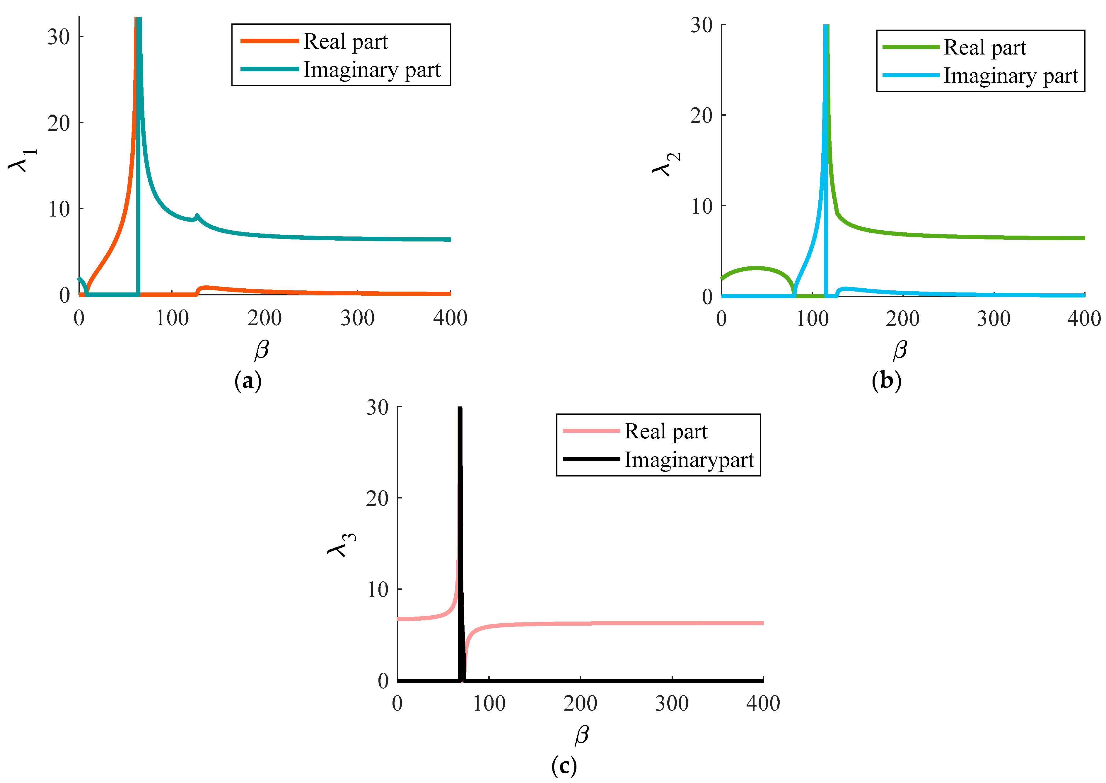
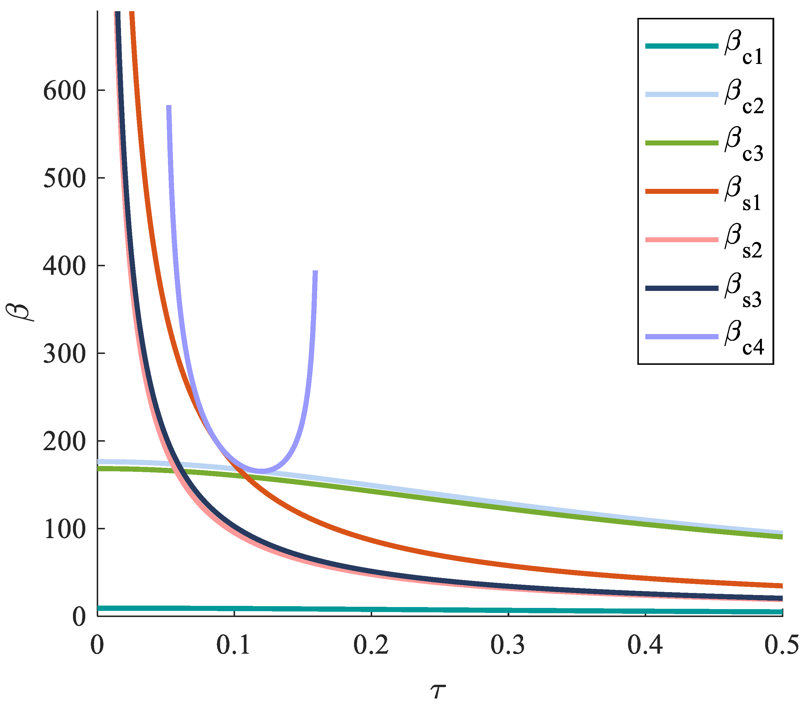
Benchmark results for the variation of the fundamental frequency parameter of a square $\left(\eta =1\right)$ thick nanosheet for six different boundary conditions are presented in

Table 2. Frequency ratio for a square plate $\left(\eta =1\right)$, different boundary conditions, thickness ratio $\left(\delta \right)$, nonlocal parameter $\left(\tau \right)$, and wave modes.

	(m = 1, n = 1)					(m = 1, n = 2)
		τ					τ
	δ	0	0.1	0.3	0.5	δ	0	0.1	0.3	0.5
SFSF	0.01	9.6270	0.9611	0.7566	0.5696	0.01	16.0971	0.9559	0.7328	0.5408
	0.1	9.4458	0.9615	0.7584	0.5717	0.1	16.0971	0.9570	0.7376	0.5460
	0.2	8.9997	0.9614	0.7580	0.5713	0.2	14.1341	0.9553	0.7308	0.5385
SCSC	0.01	28.925	0.9055	0.5787	0.3913	0.01	69.1986	0.8011	0.4060	0.2574
	0.1	26.7369	0.9069	0.5815	0.3936	0.1	59.4801	0.8059	0.4110	0.2607
	0.2	22.5099	0.9093	0.5871	0.3982	0.2	45.0569	0.8128	0.4196	0.2668
SCSF	0.01	12.6728	0.9587	0.7458	0.5568	0.01	32.9925	0.9017	0.5676	0.3804
	0.1	12.2606	0.9594	0.7487	0.5600	0.1	30.4743	0.9018	0.5680	0.3809
	0.2	11.3931	0.9587	0.7457	0.5564	0.2	25.8975	0.8998	0.5640	0.3777
SCSS	0.01	23.6327	0.9087	0.5864	0.3981	0.01	58.5687	0.8092	0.4173	0.2658
	0.1	22.4260	0.9094	0.5881	0.3995	0.1	52.3247	0.8117	0.4198	0.2675
	0.2	19.7988	0.9108	0.5914	0.4023	0.2	41.7813	0.8154	0.4244	0.2706
SFSS	0.01	11.6746	0.9564	0.7352	0.5435	0.01	27.7042	0.9057	0.5814	0.3953
	0.1	11.3810	0.9572	0.7381	0.5466	0.1	26.1910	0.9057	0.5816	0.3957
	0.2	10.7218	0.9570	0.7375	0.5459	0.2	23.2429	0.9030	0.5750	0.3898
SSSS	0.01	19.7322	0.9139	0.6001	0.4105	0.01	49.3045	0.8183	0.4287	0.2738
	0.1	19.0840	0.9139	0.6001	0.4105	0.1	45.5845	0.8183	0.4287	0.2738
	0.2	17.5055	0.9139	0.6001	0.4105	0.2	38.3847	0.8183	0.4287	0.2738
	(m = 2, n = 1)					(m = 2, n = 2)
SFSF	0.01	38.9043	0.8580	0.4844	0.3148	0.01	46.6393	0.8531	0.4748	0.3072
	0.1	36.4246	0.8588	0.4853	0.3154	0.1	42.8870	0.8543	0.4765	0.3083
	0.2	31.4338	0.8574	0.4835	0.3140	0.2	36.1646	0.8495	0.4699	0.3033
SCSC	0.01	54.6743	0.8135	0.4223	0.2691	0.01	94.3686	0.7360	0.3401	0.2120
	0.1	49.2606	0.8150	0.4240	0.2703	0.1	79.1951	0.7404	0.3437	0.2144
	0.2	40.1384	0.8165	0.4261	0.2718	0.2	59.1227	0.7448	0.3480	0.2172
SCSF	0.01	41.6472	0.8541	0.4774	0.3093	0.01	62.8595	0.8093	0.4164	0.2648
	0.1	38.7128	0.8550	0.4784	0.3099	0.1	55.9735	0.8099	0.4174	0.2655
	0.2	33.0747	0.8530	0.4757	0.3079	0.2	45.0445	0.8068	0.4137	0.2628
SCSS	0.01	51.6210	0.8156	0.4250	0.2711	0.01	85.9792	0.7414	0.3453	0.2155
	0.1	47.2245	0.8164	0.4259	0.2718	0.1	74.4019	0.7436	0.3472	0.2168
	0.2	39.2032	0.8172	0.4271	0.2726	0.2	57.3380	0.7460	0.3495	0.2183
SFSS	0.01	41.1469	0.8530	0.4754	0.3077	0.01	58.9430	0.8108	0.4441	0.2848
	0.1	38.3610	0.8540	0.4764	0.3084	0.1	53.3852	0.8111	0.4448	0.2853
	0.2	32.8922	0.8524	0.4744	0.3069	0.2	43.8579	0.8075	0.4428	0.2838
SSSS	0.01	49.3045	0.8183	0.4287	0.2738	0.01	78.8455	0.7475	0.3512	0.2196
	0.1	45.5845	0.8183	0.4287	0.2738	0.1	70.0219	0.7475	0.3512	0.2196
	0.2	38.3847	0.8183	0.4287	0.2738	0.2	55.5860	0.7475	0.3512	0.2196

for different vibrating modes $\left(\left(n, m\right)=\left(1,1\right), \left(2,1\right), \left(1,2\right), \left(2,2\right)\right)$, thickness ratios of the graphene sheet ($\delta =0.01, 0.1, 0.2)$, and nonlocal parameters ($\tau =0, 0.1, 0.3, 0.5)$. Moreover, the benchmark results for rectangular plates with $\eta =0.5$ (

Table 3. Frequency ratio for a rectangular plate with $\eta =0.5$, different boundary conditions, thickness ratio $\left(\delta \right)$, nonlocal parameter $\left(\tau \right)$, and wave modes.

	(m = 1, n = 1)					(m = 1, n = 2)
		τ					τ
	δ	0	0.1	0.3	0.5	δ	0	0.1	0.3	0.5
SFSF	0.01	9.5078	0.9644	0.7723	0.5892	0.01	27.3597	0.9557	0.7323	0.5401
	0.1	9.3306	0.9647	0.7737	0.5908	0.1	24.9711	0.9552	0.7305	0.5382
	0.2	8.9007	0.9642	0.7712	0.5878	0.2	21.3271	0.9489	0.7060	0.5113
SCSC	0.01	94.9657	0.7926	0.3957	0.2500	0.01	252.3968	0.5813	0.2309	0.1409
	0.1	75.1962	0.8009	0.4032	0.2549	0.1	166.7806	0.5988	0.2403	0.1467
	0.2	52.1283	0.8100	0.4149	0.2631	0.2	102.7371	0.6141	0.2499	0.1529
SCSF	0.01	22.7512	0.9692	0.8086	0.6758	0.01	99.3823	0.7782	0.3474	0.1914
	0.1	21.1870	0.9574	0.7992	0.6753	0.1	81.0357	0.7746	0.3509	0.1928
	0.2	18.4903	0.9592	0.7579	0.6016	0.2	57.8767	0.7771	0.3623	0.2102
SCSS	0.01	69.1986	0.8011	0.4060	0.2573	0.01	207.3996	0.5964	0.1894	0.1478
	0.1	59.4801	0.8059	0.4110	0.2607	0.1	151.1821	0.6054	0.2013	0.1507
	0.2	45.0569	0.8127	0.4196	0.2668	0.2	99.7234	0.6131	0.2507	0.1536
SFSS	0.01	16.0971	0.9559	0.7328	0.5408	0.01	75.0554	0.7998	0.4383	0.2642
	0.1	15.4054	0.9570	0.7375	0.5459	0.1	66.3720	0.7924	0.4009	0.2567
	0.2	14.1341	0.9552	0.7307	05385	0.2	52.8012	0.7831	0.3875	0.2459
SSSS	0.01	49.3045	0.8183	0.4287	0.2737	0.01	167.2821	0.6111	0.4287	0.1526
	0.1	45.5845	0.8183	0.4287	0.2737	0.1	134.3586	0.6111	0.4287	0.1526
	0.2	38.3847	0.8183	0.4287	0.2737	0.2	95.8088	0.6111	0.4287	0.1526
	(m = 2, n = 1)					(m = 2, n = 2)
SFSF	0.01	38.4774	0.8669	0.5003	0.3272	0.01	64.2036	0.8520	0.4729	0.3057
	0.1	35.9987	0.8678	0.5014	0.3281	0.1	56.5363	0.8496	0.4694	0.3029
	0.2	31.0963	0.8645	0.4963	0.3242	0.2	45.3418	0.8357	0.4491	0.2879
SCSC	0.01	115.3920	0.7293	0.3339	0.2078	0.01	275.2751	0.5553	0.2167	0.1319
	0.1	90.0396	0.7369	0.3400	0.2118	0.1	180.2276	0.5707	0.22.46	0.1369
	0.2	62.9729	0.7432	0.3463	0.2161	0.2	112.1661	0.5815	0.2311	0.1411
SCSF	0.01	50.6057	0.8599	0.4881	0.3178	0.01	131.4853	0.7207	0.3242	0.2007
	0.1	45.5725	0.8595	0.4869	0.3168	0.1	103.5900	0.7167	0.3215	0.1991
	0.2	37.5487	0.8512	0.4741	0.3069	0.2	73.0862	0.7138	0.3190	0.1976
SCSS	0.01	94.3686	0.7360	0.3401	0.2119	0.01	233.3530	0.5672	0.2239	0.1366
	0.1	79.1951	0.7404	0.3437	0.2144	0.1	167.1253	0.5753	0.2280	0.1392
	0.2	59.1227	0.7447	0.3479	0.2172	0.2	109.7471	0.6298	0.2312	0.1411
SFSS	0.01	46.6393	0.8530	0.4748	0.3072	0.01	110.5043	0.7309	0.4213	0.2603
	0.1	42.8870	0.8543	0.4765	0.3083	0.1	92.9718	0.7248	0.3860	0.2379
	0.2	36.1646	0.8495	0.4698	0.3033	0.2	69.9757	0.7156	0.3762	0.2294
SSSS	0.01	78.8455	0.7475	0.3512	0.2195	0.01	196.6991	0.5799	0.2308	0.1409
	0.1	70.0219	0.7475	0.3512	0.2196	0.1	153.5390	0.5799	0.2308	0.1409
	0.2	55.5860	0.7475	0.3512	0.2196	0.2	106.9195	0.5799	0.2308	0.1409

) and $\eta =2$ (

Table 4. Frequency ratio for a rectangular plate with $\eta =2$, different boundary conditions, thickness ratio $\left(\delta \right)$, nonlocal parameter $\left(\tau \right)$, and wave modes.

	(m = 1, n = 2)					(m = 1, n = 1)
		τ					τ
	δ	0	0.1	0.3	0.5	δ	0	0.1	0.3	0.5
SFSF	0.01	9.7328	0.9581	0.7432	0.5536	0.01	11.6746	0.9564	0.7352	0.5435
	0.1	9.5560	0.9584	0.7443	0.5547	0.1	11.3811	0.9572	0.7381	0.5466
	0.2	9.1061	0.9584	0.7444	0.5548	0.2	10.7218	0.9570	0.7375	0.5459
SCSC	0.01	13.6815	0.9417	0.6819	0.4880	0.01	23.6327	0.9087	0.5864	0.3981
	0.1	13.2843	0.9419	0.6825	0.4886	0.1	22.4260	0.9094	0.5881	0.3995
	0.2	12.3152	0.9423	0.6838	0.4898	0.2	19.7988	0.9108	0.5914	0.4023
SCSF	0.01	10.4206	0.9568	0.7372	0.5463	0.01	15.7393	0.9400	0.6757	0.4815
	0.1	10.2054	0.9572	0.7387	0.5478	0.1	15.1956	0.9406	0.6777	0.4835
	0.2	9.6782	0.9572	0.7387	0.5477	0.2	13.9934	0.9403	0.6771	0.4829
SCSS	0.01	12.9152	0.9425	0.6847	0.4909	0.01	21.5239	0.9111	0.5929	0.4039
	0.1	12.6022	0.9426	0.6850	0.4912	0.1	20.6396	0.9115	0.5937	0.4046
	0.2	11.8061	0.9428	0.7053	0.4919	0.2	18.6005	0.9122	0.6231	0.4060
SFSS	0.01	10.2948	0.9564	0.7355	0.5443	0.01	14.7549	0.9406	0.6778	0.4836
	0.1	10.0929	0.9146	0.7369	0.5456	0.1	14.3272	0.9410	0.6794	0.4853
	0.2	9.5902	0.9569	0.7371	0.5457	0.2	13.3463	0.9407	0.6786	0.4845
SSSS	0.01	12.3343	0.9435	0.6884	0.4948	0.01	19.7322	0.9139	0.6001	0.4105
	0.1	12.0752	0.9435	0.6884	0.4948	0.1	19.0840	0.9139	0.6001	0.4105
	0.2	11.3961	0.9435	0.6884	0.4948	0.2	17.5055	0.9139	0.6001	0.4105
	(m = 2, n = 1)					(m = 2, n = 1)
SFSF	0.01	39.1526	0.8528	0.4762	0.3086	0.01	41.1469	0.8530	0.4754	0.3077
	0.1	36.6824	0.8534	0.4767	0.3089	0.1	38.3610	0.8540	0.4764	0.3084
	0.2	31.6538	0.8528	0.4760	0.3084	0.2	32.8922	0.8524	0.4744	0.3069
SCSC	0.01	42.5528	0.8386	0.4564	0.2941	0.01	51.6210	0.8156	0.4250	0.2711
	0.1	39.6410	0.8388	0.4567	0.2943	0.1	47.2245	0.8164	0.4259	0.2718
	0.2	33.8397	0.8093	0.4570	0.2946	0.2	39.2032	0.8172	0.4271	0.2726
SCSF	0.01	39.7874	0.8062	0.4740	0.3069	0.01	45.0551	0.8379	0.4547	0.2926
	0.1	37.2242	0.8524	0.4746	0.3072	0.1	41.7409	0.8385	0.4554	0.2931
	0.2	32.0545	0.8517	0.4737	0.3066	0.2	35.3839	0.8375	0.4542	0.2922
SCSS	0.01	42.2071	0.8389	0.4570	0.2946	0.01	50.3833	0.8169	0.4268	0.2724
	0.1	39.3897	0.8390	0.4446	0.2947	0.1	46.3599	0.8173	0.4272	0.2727
	0.2	33.7085	0.8116	0.4439	0.2948	0.2	38.7801	0.8177	0.4278	0.2732
SFSS	0.01	39.7326	0.8215	0.4736	0.3065	0.01	44.4758	0.8382	0.3613	0.2267
	0.1	37.1858	0.8521	0.4741	0.3069	0.1	41.3217	0.8386	0.3528	0.2208
	0.2	32.0309	0.8516	0.4735	0.3051	0.2	35.1634	0.8376	0.3979	0.2518
SSSS	0.01	41.9144	0.8393	0.4576	0.2951	0.01	49.3045	0.8183	0.4287	0.2738
	0.1	39.1713	0.8393	0.4576	0.2853	0.1	45.5845	0.8183	0.4287	0.2738
	0.2	33.5896	0.8138	0.4576	0.2946	0.2	38.3847	0.8183	0.4287	0.2738

) and the same other variables of Table 2 are presented.

The benchmark results show that the lower frequency parameters correspond to the graphene sheets with less edge restraint, where the SFSF case has the lowest natural frequencies for all cases (Table 2, Table 3 and Table 4) and SCSC has the highest natural frequencies (Table 3). As the number of supported edges increases, the frequency parameters also increase. This implies that higher constraints at the edges increase the flexural rigidity of the plate, resulting in a higher frequency response. Moreover, it is observed that the frequency ratios and natural frequencies of thick graphene sheets decrease by increasing the nonlocal parameter, $\tau$, in all the cases (Table 2, Table 3 and Table 4). This, on the other hand, shows that the nonlocal effects soften graphene sheets and make them more flexible. This variation in the natural frequencies becomes more noticeable when there are more constraints on the edges. For example, the variation in the natural frequencies based on the nonlocal parameter for the SCSC boundary condition is greater than that for the SFSF boundary condition. In addition, when the number of half waves increases, this variation in natural frequencies becomes more noticeable. The thickness ratio of the graphene affects this variation in a way that by increasing the thickness ratio, the effect of the nonlocal parameter on the natural frequencies becomes more significant.

The thickness ratio of the graphene by itself has a great effect on its natural frequencies as can be seen from the benchmark results. As the thickness ratio of the graphene increases, the natural frequencies decrease for all cases. This implies that by increasing the thickness ratio of graphene, it becomes more flexible. Change in frequency due to thickness ratio is more significant when there are more constraints on the edges of the graphene. As such, the maximum change in frequency is observed in the SCSC boundary condition and the minimum change happens in the SFSF. Moreover, as the number of half waves increase, the change in natural frequency increases, so for $n=2$ and $m=2$ cases in all boundaries, there are more changes than other cases.

Additionally, as the aspect ratio of the graphene increases, the local natural frequency decreases, but it is not the same for the frequency ratio of the graphene. For example, comparing Table 2, Table 3 and Table 4 shows that by increasing the aspect ratio of the graphene with the SCSF boundary condition, the frequency ratio decreases. As the nonlocal parameter increases, the rate of change in the frequency ratio increases. However, the rate of change decreases as the aspect ratio increases. It is almost the same for SFSF and SFSS, as can be seen from Table 2, Table 3 and Table 4, but the rate of change decreases correspondingly. From Table 1, it is apparent that by increasing the aspect ratio of graphene with the SSSS boundary condition, the frequency ratio increases, either of which is in contrast with previous cases. The situation is the same for SCSS and SCSC, as can be seen from Table 1. It is observed that the free boundary condition has a significant effect on the relation between the aspect ratio and the frequency of graphene.

3.3. Wave Analysis

Waves travel in both positive and negative directions in a medium, as $\pm$ signs in Equation (15) indicate. From the dispersion relations of Equation (14), it is evident that the phase velocity $\omega /\lambda$ is frequency dependent, meaning that the plate’s waves are dispersive (they travel at different velocities at different frequencies). Also, wavenumbers (${\lambda }_i$) can be real, imaginary, or complex numbers in different frequency regions, which is based on the dispersion relations of Equation (14). Consequently, there will be different types of waves in different frequency regions such as: (i) when an exponential wave of Equation (15) has a pure imaginary argument, there is a propagating wave in the graphene; (ii) when an argument is a real number, the type of wave is evanescent; (iii) and finally, when an argument is a complex number, the wave is a decaying wave. A can be seen from Figure 3 (which is a square graphene $\left(\eta =1\right)$ of thickness ratio $\delta =0.3$ and nonlocal parameter of $\tau =0.1$), depending on frequency region all three types of waves can exist in the graphene. In this figure, it is obvious that at some frequencies, there is a wave mode transition. These frequency spots are called bifurcation frequencies and classified as cut-off and escape frequencies. Cut-off frequencies are the frequencies at which a wavenumber becomes zero, phase velocity tends to take exceptionally large values, and a qualitative change occurs in a wave mode. At escape frequencies, a wavenumber tends to take exceptionally large values, the phase velocities tend to take exceedingly small values, and a transition in wave mode occurs. These frequency spots depend on the frequency range, nonlocal parameter, thickness ratio of graphene, correction factor, and Poisson’s ratio. For a graphene sheet formulated with the first order shear deformation theory, four cut-off frequencies are derived from Equation (14) as below:

$${\beta }_{c1}={\left(\frac{-b + {\left(b^2-4ac\right)}^{\frac{1}{2}}}{2a}\right)}^{\frac{1}{2}}$$

(27a)

$${\beta }_{c2}={\left(\frac{{\left(m\pi \right)}^2\frac{1-\nu }{2} + 6k\frac{1-\nu }{{\delta }^2}}{\frac{{\delta }^2}{12} + {\tau }^2{\delta }^2\frac{{\left(m\pi \right)}^2}{12}}\right)}^{\frac{1}{2}}$$

(27b)

$${\beta }_{c3}={\left(\left(\frac{-b-{\left(b^2-4ac\right)}^{\frac{1}{2}}}{2a}\right)\right)}^{\frac{1}{2}}$$

(27c)

$${\beta }_{c4}=\frac{72k{\nu }_1{\left(-\frac{{\delta }^4{k}^2{\nu }_1^2}{9}+\frac{2{\delta }^{4}k{\nu }_1}{9}-\frac{{\delta }^4}{9}+\frac{8{\delta }^2{k}^2{\nu }_1^2{\tau }^2}{3}+\frac{8{\delta }^{2}k{\nu }_1{\tau }^2}{3}-16k^2{\nu }_1^2{\tau }^4\right)}^{\frac{1}{2}}}{{\delta }^4{k}^2{\nu }_1^2-2{\delta }^{4}k{\nu }_1+ {\delta }^4-24{\delta }^2{k}^2{\nu }_1^2{\tau }^2-24{\delta }^{2}k{\nu }_1{\tau }^2+ 144k^2{\nu }_1^2{\tau }^4}$$

(27d)

where

$$\begin{gathered} a=-{\left(m\pi \right)}^4{\tau }^4\frac{{\delta }^4}{72k\left(1-\nu \right)}+{\left(m\pi \right)}^2{\tau }^2\frac{{\delta }^4}{36k\left(-1+\nu \right)}+\frac{{\delta }^4}{72k\left(-1+\nu \right)}, \\ b=\left(\frac{1}{12}+\frac{1}{6k\left(1-\nu \right)}\right){\tau }^2{\delta }^2{\left(m\pi \right)}^4+\left(-\frac{{\delta }^2}{6k\left(-1+\nu \right)}+\frac{12{\tau }^2+{\delta }^2}{12}\right){\left(m\pi \right)}^2+1 \end{gathered}$$

(28)

and three escape frequencies as

$${\beta }_{s1}={\left(6k\frac{1-\nu }{{\tau }^2{\delta }^2}\right)}^{\frac{1}{2}}$$

(29a)

$${\beta }_{s2}={\left(6\frac{1-\nu }{{\tau }^2{\delta }^2}\right)}^{\frac{1}{2}}$$

(29b)

$${\beta }_{s3}={\left(\frac{12}{{\tau }^2{\delta }^2}\right)}^{\frac{1}{2}}$$

(29c)

where the subscripts “c” and “s” stand for cut-off frequency and escape frequency, respectively.

By dividing the frequency range into frequency intervals based on these bifurcation frequencies, different waves in a medium can be found. For the graphene of Figure 3, the frequency region can be divided into eight regions as: 0$<\beta <{\beta }_{c1}, {\beta }_{c1}<\beta <{\beta }_{s1}, {\beta }_{s1}<\beta <{\beta }_{s2},{\beta }_{s2}<\beta <{\beta }_{c2},{\beta }_{c2}<\beta <{\beta }_{c3},{\beta }_{c3}<\beta <{\beta }_{s3}, {\beta }_{s3}<\beta <{\beta }_{c4},$ and $\beta >{\beta }_{c4}$. In the $0<\beta <{\beta }_{c1}$ frequency region, three evanescent waves exist in the medium as all arguments of the Equation (15) are real values. In the next frequency region, ${\beta }_{c1}<\beta <{\beta }_{s1}$, the first wave, with ${\lambda }_1$ wavenumber, has a pure imaginary argument and is a propagating wave and the other two waves are evanescent. After ${\beta }_{s1}$ and in the ${\beta }_{s1}<\beta <{\beta }_{s2}$ region, again the first wave changes to an evanescent wave. At the second escape frequency, ${\beta }_{s2}$, a qualitative change occurs in the third wave and in the ${\beta }_{s2}<\beta <{\beta }_{c2}$ region, this wave is a propagating wave and the first and second waves are evanescent waves. In the fifth frequency region, ${\beta }_{c2}<\beta <{\beta }_{c3}$, the third wave again changes into an evanescent wave. In the sixth frequency region, ${\beta }_{c2}<\beta <{\beta }_{s3}$, the second wave becomes a propagating wave while the other two waves are evanescent. In the ${\beta }_{s3}<\beta <{\beta }_{c4}$ region again, this wave changes into an evanescent wave and the other two waves remain evanescent. Finally, in the high frequency range, after the last cut-off frequency, the first and second waves have both imaginary and real parts in their arguments, complex values, so the waves are decaying type in this region. However, this division of the frequency range and the order of bifurcation frequencies are not unique, and they may change by changing the nonlocal parameter and the thickness ratio of graphene as discussed in the next sections.

3.3.1. Effect of Nonlocal Parameter on Wave Motion

To investigate the effect of nonlocal parameter on these bifurcation frequencies, they are depicted in Figure 4 for a $\delta =0.2, \eta =0.6, \nu =0.3, k=0.86667$ plate, $\left(n,m\right)=\left(1.1\right)$ wave mode, and varying nonlocal parameter (horizontal axis). Interesting features are captured for these important frequencies. First, it is interesting that the occurrence of ${\beta }_{c4}$ depends on the value of the nonlocal parameter, meaning this cut-off frequency appears only for some specific values (in a specific interval) of the nonlocal parameter. Lower and upper values of this interval are derived analytically as follows:

$${\tau }_{cr1},{\tau }_{cr2}={\left(\frac{8{\delta }^2{k}^2{\nu }_1^2\pm 3{\delta }^2{\left(\frac{256k^3{\nu }_1^3}{9}\right)}^{\frac{1}{2}}+ 8{\delta }^{2}k{\nu }_1}{96k^2{\nu }_1^2}\right)}^{\frac{1}{2}}$$

(30)

which, as can be seen, depend on thickness ratio, shear correction factor, and Poisson’s ratio.

Therefore, in the ${\tau }_{cr1}<\tau <{\tau }_{cr2}$ range, which we call its lower and higher values critical nonlocal parameters, there are four cut-off frequencies and out of this range, there are three cut-off frequencies and the fourth, ${\beta }_{c4}$, does not appear; there are three escape frequencies everywhere.

Moreover, the highest bifurcation frequency is ${\beta }_{c4}$ (if it exists), and the lowest always is ${\beta }_{c1}$ for different nonlocal parameters. As mentioned in the previous section, it is evident from Figure 3 that before the lowest cut-off frequency, all three waves are evanescent waves. However, for the high frequency range after the highest bifurcation frequency, there are three scenarios. The first scenario is the case that the highest bifurcation frequency is ${\beta }_{c4}$. In this case, the first and second waves of Equation (15) become decaying waves after this cut-off frequency where there are propagating components in these two waves. Second, two scenarios happen when the graphene’s nonlocal parameter is out of critical range and the highest bifurcation frequency is either ${\beta }_{c2}$ or ${\beta }_{s1}$. As seen from Figure 4, for a specific value of nonlocal parameter, there is an intersection between ${\beta }_{c2}$ and ${\beta }_{s1}$ which results in a change in their order. This intersection is obtained analytically in the Appendix A. In these two cases, whether the highest bifurcation frequency is ${\beta }_{c2}$ or ${\beta }_{s1}$, after the highest bifurcation frequency, all waves are evanescent waves where their energy decays in the direction of ongoing waves. There are other intersections of ${\beta }_{c2}$ and ${\beta }_{c3}$ with ${\beta }_{s1}, {\beta }_{s2}$, and ${\beta }_{s3}$, which are also analytically derived in Appendix A. In each of these intersections, the order of the two intersected bifurcation frequencies changes. No intersections between cut-off frequencies nor between escape frequencies are captured. Moreover, in two frequency spots, ${\beta }_{c4}$ becomes very close to ${\beta }_{c2}$ and ${\beta }_{s1}$.

Figure 4 also shows that as the nonlocal parameter tends to zero, which on the other hand means tending to the classical/local Mindlin plate theory, the escape frequencies tend to very large values which are considered unreachable. Therefore, for very small values of nonlocal parameter, there are three cut-off frequencies in the realistic frequency range, which is in agreement with previous studies [54].

3.3.2. Effect of Graphene’s Thickness Ratio on Wave Motion

Figure 5 shows the variation of bifurcation frequency versus thickness ratio for graphene of $\tau =0.1, \eta =0.6, \nu =0.3, k=0.86667$, and $m=1$. From this figure, it also can be seen that ${\beta }_{c4}$ happens only in a specific region of $\delta$. This region’s lower and upper frequencies are found analytically as:

$${\delta }_{cr1},{\delta }_{cr2}={\left(\frac{3\left(8k{\nu }_1{\xi }^2\pm 3{\xi }^2{\left(\frac{256k^3{\nu }_1^3}{9}\right)}^{\frac{1}{2}}+ 8k^2{\nu }_1^2{\xi }^2\right)}{2\left(k^2{\nu }_1^2-2k{\nu }_1+ 1\right)}\right)}^{\frac{1}{2}}$$

(31)

Therefore, if the thickness ratio of the graphene is in the ${\delta }_{cr1}<\delta <{\delta }_{cr2}$ range, there will be four cut-off frequencies, and if there are three cut-offs out of this frequency range, there will be three escape frequencies for every thickness ratio.

Moreover, regarding the highest and lowest bifurcation frequencies, it can be seen in Figure 5 that the lowest frequency is always ${\beta }_{c1}$, below which all the three ongoing waves are evanescent. Like the nonlocal parameter effect, there are also three scenarios for the thickness ratio effect when it comes to high frequency region. In the presence of ${\beta }_{c4}$, this cut-off frequency is the highest frequency. However, in cases where this bifurcation does not occur in the medium, the highest frequency can be ${\beta }_{c2}$ or ${\beta }_{s1}$, depending on the thickness ratio. Evident from Figure 5, there is an intersection between these two bifurcation frequencies, which is derived analytically in Appendix B. Considering this intersection and whether the thickness ratio is less or greater than this intersection, the highest frequency can be defined. There are other intersections of ${\beta }_{c2}$ and ${\beta }_{c3}$ with ${\beta }_{s1}, {\beta }_{s2}$, and ${\beta }_{s3}$, which are also analytically derived in Appendix B. Moreover, in two frequency spots, ${\beta }_{c4}$ becomes remarkably close to ${\beta }_{c2}$ and ${\beta }_{s1}$. At each of these intersections, the order of the two intersected bifurcation frequencies changes. There is not any intersection between cut-off frequencies nor between escape frequencies. Therefore, their order will not change by varying thickness ratio of the plate.

4. Conclusions

This paper employs wave propagation techniques and Mindlin graphene sheet theory to present an exact solution for the free vibration analysis of thick rectangular graphene sheets. There are other analytical solutions in the literature, but this is the first time that the effects of thickness ratio and nonlocal parameter have been considered. The proposed wave propagation method showed high accuracy and reliability in both macro and nanoscales. The exact characteristic equations are derived for six boundary condition cases having two opposite sides simply supported. The six cases considered are namely SSSS, SCSS, SCSC, SSSF, SFSF, and SCSF plates. The proposed method showed excellent accuracy in comparison with literature. Frequency parameter benchmark results are presented for different nonlocal parameters, thickness ratios, aspect ratios, and number of half waves for each case. These frequency parameters can be deemed as a database for each of the considered cases and used to investigate the accuracy of computational methods for graphene sheets. Moreover, cut-off and escape frequencies are found analytically, which offers us to investigate the bifurcation frequencies more in detail. Four cut-off frequencies are observed, among which one of them occurs only in a specific range of nonlocal parameter and thickness ratio of the plate, so in these ranges, there are four cut-off and three escape frequencies and out of these ranges there are three cut-off and three escape frequencies. Additionally, the lowest bifurcation frequency is always a cut-off frequency, but the highest bifurcation frequency can be a cut-off or escape frequency depending on the nonlocal parameter and thickness ratio of the graphene sheet. There are changes in the order of escape and cut-off frequencies, which are captured and derived analytically.

References

1. Chen, Z.; Zhang, C.; Wu, Q.; Li, K.; Tan, L. Application of triangular silver nanoplates for colorimetric detection of H2O2. Sens. Actuators B Chem. 2015, 220, 314–317. [Google Scholar] [CrossRef]
2. Walkey, C.; Sykes, E.A.; Chan, W.C.W. Application of semiconductor and metal nanostructures in biology and medicine. Hematology 2009, 2009, 701–707. [Google Scholar] [CrossRef] [PubMed]
3. La, D.D.; Nguyen, T.A.; Nguyen, T.T.; Ninh, H.D.; Thi, H.P.N.; Nguyen, T.T.; Nguyen, D.A.; Dang, T.D.; Rene, E.R.; Chang, S.W.; et al. Absorption Behavior of Graphene Nanoplates toward Oils and Organic Solvents in Contaminated Water. Sustainability 2019, 11, 7228. [Google Scholar] [CrossRef]
4. Lin, S.; Lu, Y.; Xu, J.; Feng, S.; Li, J. High performance graphene/semiconductor van der Waals heterostructure optoelectronic devices. Nano Energy 2017, 40, 122–148. [Google Scholar] [CrossRef]
5. Bykkam, S.; Prasad, D.; Maurya, M.; Sadasivuni, K.; Cabibihan, J.-J. Comparison Study of Metal Oxides (CeO2, CuO, SnO2, CdO, ZnO and TiO2) Decked Few Layered Graphene Nanocomposites for Dye-Sensitized Solar Cells. Sustainability 2021, 13, 7685. [Google Scholar] [CrossRef]
6. Guo, T.; Fu, H.; Wang, C.; Chen, H.; Chen, Q.; Wang, Q.; Chen, Y.; Li, Z.; Chen, A. Road Performance and Emission Reduction Effect of Graphene/Tourmaline-Composite-Modified Asphalt. Sustainability 2021, 13, 8932. [Google Scholar] [CrossRef]
7. Wang, L.; Loh, K.J.; Mousacohen, R.; Chiang, W.-H. Printed Graphene-Based Strain Sensors for Structural Health Monitoring. Asme Conf. Smart Mater. 2017. [Google Scholar] [CrossRef]
8. Sankar, V.; Nambi, A.; Bhat, V.N.; Sethy, D.; Balasubramaniam, K.; Das, S.; Guha, M.; Sundara, R. Waterproof Flexible Polymer-Functionalized Graphene-Based Piezoresistive Strain Sensor for Structural Health Monitoring and Wearable Devices. ACS Omega 2020, 5, 12682–12691. [Google Scholar] [CrossRef]
9. Morsin, M.; Salleh, M.M.; Umar, A.A.; Sahdan, M.Z. Gold Nanoplates for a Localized Surface Plasmon Resonance-Based Boric Acid Sensor. Sensors 2017, 17, 947. [Google Scholar] [CrossRef]
10. Xu, C.; Qu, J.; Rong, D.; Zhou, Z.; Leung, A. Theory and modeling of a novel class of nanoplate-based mass sensors with corner point supports. Thin-Walled Struct. 2021, 159, 107306. [Google Scholar] [CrossRef]
11. Acharyya, S.; Manna, B.; Nag, S.; Guha, P.K. WO3 Nanoplates Based Chemiresistive Sensor Device for Selective Detection of 2-Propanol. In Proceedings of the IEEE SENSORS, Montreal, QC, Canada, 27–30 October 2019; pp. 1–4. [Google Scholar] [CrossRef]
12. Yang, Z.; Pang, Y.; Han, X.-L.; Yang, Y.; Ling, J.; Jian, M.; Zhang, Y.; Yang, Y.; Ren, T.-L. Graphene Textile Strain Sensor with Negative Resistance Variation for Human Motion Detection. ACS Nano 2018, 12, 9134–9141. [Google Scholar] [CrossRef]
13. Trung, T.Q.; Lee, N.-E. Flexible and Stretchable Physical Sensor Integrated Platforms for Wearable Human-Activity Monitoringand Personal Healthcare. Adv. Mater. 2016, 28, 4338–4372. [Google Scholar] [CrossRef] [PubMed]
14. Chen, S.; Jiang, K.; Lou, Z.; Chen, D.; Shen, G. Recent Developments in Graphene-Based Tactile Sensors and E-Skins. Adv. Mater. Technol. 2018, 3, 1700248. [Google Scholar] [CrossRef]
15. Liu, T.-C.; Chuang, M.-C.; Chu, C.-Y.; Huang, W.-C.; Lai, H.-Y.; Wang, C.-T.; Chu, W.-L.; Chen, S.-Y.; Chen, Y.-Y. Implantable Graphene-based Neural Electrode Interfaces for Electrophysiology and Neurochemistry in In Vivo Hyperacute Stroke Model. ACS Appl. Mater. Interfaces 2016, 8, 187–196. [Google Scholar] [CrossRef] [PubMed]
16. Yang, T.; Jiang, X.; Zhong, Y.; Zhao, X.; Lin, S.; Li, J.; Li, X.; Xu, J.; Li, Z.; Zhu, H. A Wearable and Highly Sensitive Graphene Strain Sensor for Precise Home-Based Pulse Wave Monitoring. ACS Sens. 2017, 2, 967–974. [Google Scholar] [CrossRef]
17. Huang, H.; Su, S.; Wu, N.; Wan, H.; Wan, S.; Bi, H.; Sun, L. Graphene-Based Sensors for Human Health Monitoring. Front. Chem. 2019, 7, 399. [Google Scholar] [CrossRef]
18. Rapaport, D.C. The Art of Molecular Dynamics Simulation, 2nd ed.; Cambridge University Press: Cambridge, UK, 2004. [Google Scholar] [CrossRef]
19. Nazemnezhad, R.; Zare, M.; Hosseini-Hashemi, S. Sandwich plate model of multilayer graphene sheets for considering interlayer shear effect in vibration analysis via molecular dynamics simulations. Appl. Math. Model. 2017, 47, 459–472. [Google Scholar] [CrossRef]
20. Legoas, S.B.; Coluci, V.R.; Braga, S.F.; Coura, P.Z.; Dantas, S.O.; Galvão, D.S. Molecular-Dynamics Simulations of Carbon Nanotubes as Gigahertz Oscillators. Phys. Rev. Lett. 2003, 90, 055504. [Google Scholar] [CrossRef] [Green Version]
21. John, T.; Thomas, T.; Abel, B.; Wood, B.R.; Chalmers, D.K.; Martin, L.L. How kanamycin A interacts with bacterial and mammalian mimetic membranes. Biochim. Et Biophys. Acta (BBA) Biomembr. 2017, 1859, 2242–2252. [Google Scholar] [CrossRef]
22. Fu, T.; Mao, Y.; Tang, Y.; Zhang, Y.; Yuan, W. Effect of nanostructure on rapid boiling of water on a hot copper plate: A molecular dynamics study. Heat Mass Transf. 2016, 52, 1469–1478. [Google Scholar] [CrossRef]
23. Sahmani, S.; Fattahi, A.M. Development of efficient size-dependent plate models for axial buckling of single-layered graphene nanosheets using molecular dynamics simulation. Microsyst. Technol. 2017, 24, 1265–1277. [Google Scholar] [CrossRef]
24. Yang, X.; Zhou, T.; Chen, C. Effective elastic modulus and atomic stress concentration of single crystal nano-plate with void. Comput. Mater. Sci. 2007, 40, 51–56. [Google Scholar] [CrossRef]
25. Sarayi, S.M.M.J.; Faghihi, D.; Waqas, M.; Siddiqui, A.H.; Tutino, V.M. A Hybrid Finite Element and Smoothed-Particle Hydrodynamics Method Can Simulate Peri-Procedural Complications of Thrombectomy. Circulation 2022, 144, A14359. Available online: https://www.ahajournals.org/doi/abs/10.1161/circ.144.suppl_1.14359 (accessed on 24 August 2022).
26. Cemal, A. Eringen, Nonlocal Continuum Field Theories; Springer: New York, NY, USA, 2002. [Google Scholar] [CrossRef]
27. Peddieson, J.; Buchanan, G.R.; McNitt, R.P. Application of nonlocal continuum models to nanotechnology. Int. J. Eng. Sci. 2003, 41, 305–312. [Google Scholar] [CrossRef]
28. Aydogdu, M. Axial vibration of the nanorods with the nonlocal continuum rod model. Phys. E Low-Dimens. Syst. Nanostructures 2009, 41, 861–864. [Google Scholar] [CrossRef]
29. Lei, Z.; Zhang, L.; Liew, K.; Yu, J. Dynamic stability analysis of carbon nanotube-reinforced functionally graded cylindrical panels using the element-free kp-Ritz method. Compos. Struct. 2014, 113, 328–338. [Google Scholar] [CrossRef]
30. Zhang, L.; Zhang, Y.; Liew, K. Vibration analysis of quadrilateral graphene sheets subjected to an in-plane magnetic field based on nonlocal elasticity theory. Compos. Part B Eng. 2017, 118, 96–103. [Google Scholar] [CrossRef]
31. Pradhan, S.; Phadikar, J. Nonlocal elasticity theory for vibration of nanoplates. J. Sound Vib. 2009, 325, 206–223. [Google Scholar] [CrossRef]
32. Phadikar, J.; Pradhan, S. Variational formulation and finite element analysis for nonlocal elastic nanobeams and nanoplates. Comput. Mater. Sci. 2010, 49, 492–499. [Google Scholar] [CrossRef]
33. Aghababaei, R.; Reddy, J. Nonlocal third-order shear deformation plate theory with application to bending and vibration of plates. J. Sound Vib. 2009, 326, 277–289. [Google Scholar] [CrossRef]
34. Namin, S.A.; Pilafkan, R. Vibration analysis of defective graphene sheets using nonlocal elasticity theory. Phys. E Low-Dimens. Syst. Nanostructures 2017, 93, 257–264. [Google Scholar] [CrossRef]
35. Hashemi, S.H.; Zare, M.; Nazemnezhad, R. An exact analytical approach for free vibration of Mindlin rectangular nano-plates via nonlocal elasticity. Compos. Struct. 2013, 100, 290–299. [Google Scholar] [CrossRef]
36. Sarrami-Foroushani, S.; Azhari, M. Nonlocal vibration and buckling analysis of single and multi-layered graphene sheets using finite strip method including van der Waals effects. Phys. E Low-Dimens. Syst. Nanostructures 2014, 57, 83–95. [Google Scholar] [CrossRef]
37. Hosseini-Hashemi, S.; Kermajani, M.; Nazemnezhad, R. An analytical study on the buckling and free vibration of rectangular nanoplates using nonlocal third-order shear deformation plate theory. Eur. J. Mech. A/Solids 2015, 51, 29–43. [Google Scholar] [CrossRef]
38. Patel, P.; Sarayi, S.M.M.J.; Chen, D.; Hammond, A.L.; Damiano, R.J.; Davies, J.M.; Xu, J.; Meng, H. Fast virtual coiling algorithm for intracranial aneurysms using pre-shape path planning. Comput. Biol. Med. 2021, 134, 104496. [Google Scholar] [CrossRef]
39. Charvade, A.S.; Sarayi, S.M.M.J. An Analytical Approach for Preliminary Response-Based Design of Semi Rigid Moment Resisting Frames. Prog. Appl. Sci. Eng. 2021, 6. Available online: https://www.crpase.com/viewmore.php?pid=174 (accessed on 24 August 2022).
40. Eftekhar, S.; Sarayi, S.M.M.J. An analytical solution for nonlinear dynamics of one kind of scanning probe microscopes. arXiv 2020, arXiv:2009.05600. [Google Scholar]
41. Mei, C.; Mace, B.R. Wave Reflection and Transmission in Timoshenko Beams and Wave Analysis of Timoshenko Beam Structures. J. Vib. Acoust. 2004, 127, 382–394. [Google Scholar] [CrossRef]
42. Tan, C.; Kang, B. Wave reflection and transmission in an axially strained rotating Timoshenko shaft. J. Sound Vib. 1998, 213, 483–510. [Google Scholar] [CrossRef]
43. Lee, S.-K.; Mace, B.; Brennan, M. Wave propagation, reflection and transmission in non-uniform one-dimensional waveguides. J. Sound Vib. 2007, 304, 31–49. [Google Scholar] [CrossRef]
44. Mei, C.; Karpenko, Y.; Moody, S.; Allen, D. Analytical approach to free and forced vibrations of axially loaded cracked Timoshenko beams. J. Sound Vib. 2006, 291, 1041–1060. [Google Scholar] [CrossRef]
45. Mei, C. In-plane Vibrations of Classical Planar Frame Structures? an Exact Wave-based Analytical Solution. J. Vib. Control 2010, 16, 1265–1285. [Google Scholar] [CrossRef]
46. Mei, C. Studying the effects of lumped end mass on vibrations of a Timoshenko beam using a wave-based approach. J. Vib. Control 2012, 18, 733–742. [Google Scholar] [CrossRef]
47. Mei, C. Free vibration analysis of classical single-story multi-bay planar frames. J. Vib. Control 2013, 19, 2022–2035. [Google Scholar] [CrossRef]
48. Bahrami, M.N.; Arani, M.K.; Saleh, N.R. Modified wave approach for calculation of natural frequencies and mode shapes in arbitrary non-uniform beams. Sci. Iran. 2011, 18, 1088–1094. [Google Scholar] [CrossRef]
49. Bahrami, A.; Teimourian, A. Study on vibration, wave reflection and transmission in composite rectangular membranes using wave propagation approach. Meccanica 2017, 1–19. [Google Scholar] [CrossRef]
50. Bahrami, A.; Teimourian, A. Nonlocal scale effects on buckling, vibration and wave reflection in nanobeams via wave propagation approach. Compos. Struct. 2015, 123, 1061–1075. [Google Scholar] [CrossRef]
51. Bahrami, A. A wave-based computational method for free vibration, wave power transmission and reflection in multi-cracked nanobeams. Compos. Part B Eng. 2017, 120, 168–181. [Google Scholar] [CrossRef]
52. Bahrami, A. Free vibration, wave power transmission and reflection in multi-cracked nanorods. Compos. Part B Eng. 2017, 127, 53–62. [Google Scholar] [CrossRef]
53. Bahrami, A.; Teimourian, A. Small scale effect on vibration and wave power reflection in circular annular nanoplates. Compos. Part B Eng. 2017, 109, 214–226. [Google Scholar] [CrossRef]
54. Sarayi, S.M.M.J.; Bahrami, A.; Bahrami, M.N. Free vibration and wave power reflection in Mindlin rectangular plates via exact wave propagation approach. Compos. Part B Eng. 2018, 144, 195–205. [Google Scholar] [CrossRef]
55. Sarayi, S.M.M.J.; Damiano, R.J.; Patel, P.; Dargush, G.; Siddiqui, A.H.; Meng, H. A Nonlinear Mechanics-based Virtual Coiling Method For Intracranial Aneurysm. Summer Biomech. Bioeng. Biotransport Conf. 2020. [Google Scholar] [CrossRef]
56. Zitoun, A.; Fakis, D.; Jayasree, N.; Omairey, S.; Oikonomidis, F.; Stoeva, Z.; Kazilas, M. Graphene-based strain sensing in composites for structural and health monitoring applications. SN Appl. Sci. 2022, 4, 1–17. [Google Scholar] [CrossRef]
57. Bahrami, A.; Teimourian, A. Study on the effect of s. mall scale on the wave reflection in carbon nanotubes using nonlocal Timoshenko beam theory and wave propagation approach. Compos. B Eng. 2016, 91, 492–504. [Google Scholar] [CrossRef]
58. Mindlin, R.D. Influence of Rotatory Inertia and Shear on Flexural Motions of Isotropic, Elastic Plates. J. Appl. Mech. 2021, 18, 31–38. [Google Scholar] [CrossRef]
59. Samaei, A.; Abbasion, S.; Mirsayar, M. Buckling analysis of a single-layer graphene sheet embedded in an elastic medium based on nonlocal Mindlin plate theory. Mech. Res. Commun. 2011, 38, 481–485. [Google Scholar] [CrossRef]
Figure 1. Wave presentation on a thick graphene sheet.
Sustainability 14 12329 g001
Figure 2. Real and Imaginary parts of characteristic equation.
Sustainability 14 12329 g002
Figure 3. Dispersion relations for three wavenumbers of graphene sheet based on nonlocal frequency: (a) First wavenumber ( λ 1 ) versus frequency; (b) second wavenumber ( λ 2 ) versus frequency; (c) third wavenumber ( λ 2 ) versus frequency.
Sustainability 14 12329 g003
Figure 4. Bifurcation frequencies variation with dimensionless nonlocal parameter.
Sustainability 14 12329 g004
Figure 5. Bifurcation frequencies variation with thickness ratio of plate.
Sustainability 14 12329 g005