Scale-Location Dependence Relationship between Soil Organic Matter and Environmental Factors by Anisotropy Analysis and Multiple Wavelet Coherence

Abstract

Soil organic matter (SOM) and environmental factors have been shown to have a scale-location dependence relationship. However, few studies have considered the anisotropy, and the scale-location dependence relationship may not be fully characterized. In this study, transects with dominant directions of SOM variability in the dryland farming regions of Songliao Plain, China were extracted by anisotropy analysis. The scale-location specific multivariate relationships between SOM and environmental factors along the two transects were examined using multiple wavelet coherence. Results indicated that the scale and location-specific variations in SOM and environmental factors were direction-specific. The major direction with the most significant SOM variations was 56° east by north, while the minor direction was perpendicular to the major direction. The strongest single factor for explaining SOM variations differed between two dominant directions, sand along the major direction (average wavelet coherence (AWC) = 0.57, percentage area of significant coherence (PASC) = 40.32% at all scales) and bulk density (BD) along the minor direction (AWC = 0.66, PASC = 50.16% at all scales). The combination of mean annual temperature (MAT) and BD was the best to explain SOM variations along the major direction (AWC = 0.78, PASC = 46.23% at all scales). A two-factor combination is adequate to explain SOM variability along the major direction, whereas a single factor is sufficient for the explanation along the minor direction. More factors did not evidently increase or even decrease the percentage of scale-location domains where SOM variations were significantly explained. This work has important implications for developing future sampling strategies and preparing detailed digital soil maps.

1. Introduction

Soil organic matter (SOM) is one of the key factors used for characterizing soil fertility and quality [1]. SOM is a major form of carbon sink and source and plays an important role in terrestrial carbon dynamics and climate change mitigation [2]. Adequate understanding of the spatial distribution of SOM is critical for SOM prediction, terrestrial carbon cycle simulation, and soil quality assessment [3].

The spatial distribution of SOM exhibits great heterogeneity at global, regional, local, and field scales [4,5,6], which is influenced by a range of environmental factors that operate at different scales with different intensities. Accordingly, the spatial variation of SOM with environmental factors is related to scale and location. Therefore, it is necessary to understand how environmental factors affect the variability of SOM at different scales and locations.

Numerous methods, such as Fourier transform (FT) [7,8], wavelet transform (WT) [9,10], and empirical mode decomposition (EMD) [11,12] have been applied to reveal the scale and location-specific relationship between a soil property and an individual environmental factor. However, geoscientific processes are often complex and may be influenced by multiple environmental factors, so simultaneously, a single factor may not fully explain SOM variability [13,14]. Over the past decade, several approaches have been employed to analyze multivariate relationships at various scales, such as multiple spectral coherence (MSC) [15,16] and multivariate empirical mode decomposition (MEMD) [17,18,19]. However, the aforementioned methods mainly target the multiscale variations of soil properties and are unable to reveal soil properties variations at different locations simultaneously. Multiple wavelet coherence (MWC) was established to resolve multivariate (≥3 variables) relationships at various scales and locations [20]. In contrast to common multivariate approaches, MWC has shown superior performance in quantifying multivariate relations in the geosciences with scale-location dependence [21,22].

MWC characterizes the scale and location-specific features by partitioning spatial series into scales and locations. Such spatial series are usually collected along a transect selected from the study area. Anisotropy is unavoidable as the SOM variability may be dominated by specific directions [23,24]. By fitting a model to spatial correlation or continuity, variograms show different lengths in different directions. Directional variograms are used to assess the degree of anisotropy and the major and minor directions along the variogram ranges that are expected to be the longest and smallest, respectively [25]. The representative transects can be identified using various anisotropy analysis (AA) methods [9]. One method is to calculate the spatial dependence along different orientations in polar coordinates, allowing exact significance testing [26]. Alternatively, the semivariogram of the target attributes in different directions can be calculated and ellipses are used to fit these ranges. The direction of the major and the minor range of the ellipse represent the longest and the shortest distances of autocorrelation, respectively. Both approaches illustrate the spatial dependence in different forms, providing information on the variations in different directions.

In recent studies, MWC has been used to reveal the scale-location dependence relationship between SOM and multivariate [27,28,29]. However, few studies have considered the anisotropy, and the scale-location dependence relationship may not be fully characterized. The objectives of this study were to (1) explore the dominant directions of SOM variations in dryland farming regions of Songliao Plain, China, using AA; (2) characterize the anisotropy and scale-location dependent relationships between SOM and environmental factors using MWC; and (3) identify principal factors for the variations of SOM in the dominant directions at different scales and locations. This study has important implications for the development of future sampling strategies and the preparation of detailed digital soil maps.

2. Materials and Methods

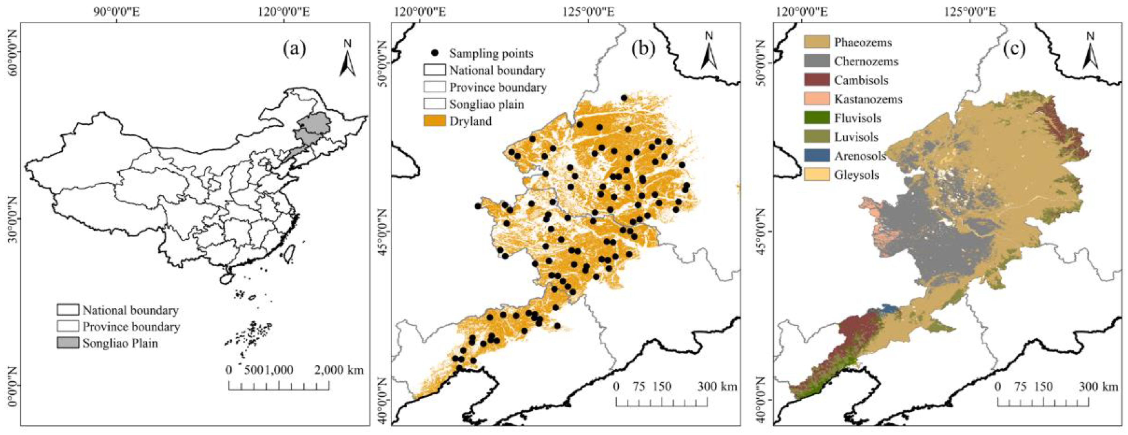
2.1. Study Area

The study was carried out in the dryland located in the Songliao Plain, China (between 39–49° N and 119–128° E), which covers a total of 133 districts and counties with an area of approximately 25.57 × 104 km² (Figure 1). The dryland refers to the region with a topographic slope of <5° and >40% of the cultivated land in a 1 km2 grid. The terrain of the study area consists mainly by piedmont diluvial, alluvial plains, and terraces, with altitudes ranging from 50 to 300 m. The area is dominated by a warm-temperate continental monsoon climate. The annual temperature changes between 3 and 8 °C. The annual precipitation varies from 400 to 750 mm, with 60–65% of precipitation occurring in June, July, and August. The major soil types in the study area are Phaeozems, Chernozems, and Cambisols, according to the World Reference Base for Soil Resources (WRB). The primary cropping system in the study area is monoculture.

2.2. Field Sampling and Environmental Data Collection

The Digital Elevation Model (DEM) (http://www.gscloud.cn/, (accessed on 5 June 2021)) and land-use map in 2015 (https://www.resdc.cn/, (accessed on 12 April 2020)) were overlaid to select dryland farming patches. The maps of dryland farming patches and soil types were spatially joined. The sampling sites were established to ensure the following criteria: (1) each major soil type and sub-category were covered, (2) each district and county were included with at least one sampling site, and (3) all clay content degrees had sampling sites distributed.

At each sampling site, the top 20 cm layer of soil was sampled, and a composite sample was obtained by mixing soil from five points. A total of 107 composite soil samples were collected in April 2017 (Figure 1), which were air dried and sieved to <2 mm. In addition, three soil cores were taken using an undisturbed soil sampler (100 cm3 in volume) and dried at 105 °C for 48 h until a constant weight was reached to measure bulk densities (BD). Sand content (0.05–2.0 mm), silt content (0.002–0.05 mm), and clay content (<0.002 mm) were determined by laser diffraction using LS-909E (Omec Instruments Co., Ltd., Zhuhai, China). The SOM was measured using the potassium dichromate oxidation method.

Various environmental factors, including topography, climate, vegetation, and edaphic attributes, were considered to assess their effects on SOM. Topographic attributes such as elevation, slope, and topographic wetness index (TWI) were included. Elevation was obtained from the DEM with a resolution of 30 m. Slope was extracted using ArcGIS 10.8 (ESRI, Inc., USA), while TWI was calculated by SAGA GIS software (http://www.passagesoftware.net/index.php, (accessed on 21 July 2020)). Climatic attributes such as mean annual temperature (MAT) and mean annual precipitation (MAP) were included. A total of 62 weather stations were scattered across the study area, which records daily temperatures and precipitations via ground observations. These data were obtained from the China Meteorological Data Service Centre (http://cdc.nmic.cn, (accessed on 5 November 2020)). Continuous surface data of MAT and MAP in 2017 were interpolated across the study area through the inverse distance weighting (IDW) method. Vegetative attributes such as normalized difference vegetation index (NDVI) and net primary productivity (NPP) were included. Landsat-8 data in 2017 with 30 m resolution was provided by the Geospatial Data Cloud site (http://www.gscloud.cn/, (accessed on 3 September 2021)), and NDVI was extracted using ENVI 5.1 (ESRI Inc, USA). The NPP data were calculated from the 2017 MOD17A3HGF dataset at 500 m and the spatial resolution was provided by NASA (https://ladsweb.modaps.eosdis.nasa.gov/, (accessed on 3 September 2021)). Edaphic attributes, including sand content, clay content, and BD, were derived from the laboratory analyses as mentioned in the previous. Environmental factors that did not meet the resolution of 30 m were processed to the same grid.

2.3. Transect Establishment

The measured SOM was interpolated onto a 30 m grid by the IDW method, with the cross-validation determination coefficient of 0.53 (Figure 2). Anisotropy was modeled by an ellipse, whose major and minor axes represent the longest (major range) and shortest distance (minor range) to reach the sill [30]. The major range and minor ranges of semivariograms in different directions were identified using the Geostatistical Analyst Tool embedded in ArcGIS 10.8. The major and minor ranges of the SOM were along the east by north 56° (S1) and 146° (S2), respectively. The S1 axis is oriented in the same direction as the major ranges of the Greater Khingan and Changbai Mountains. Following the identification of the major and minor ranges, two representative transects were constructed and were resampled at 1 km sampling intervals. One transect (S1) was 495 km long along the major axis with 495 sampling points. The other transect (S2) was 280 km long along the minor axis with 280 sampling points. The SOM and environmental factors were extracted from each sampling point.

2.4. MWC and BWC

The MWC method is an extension of bivariate wavelet coherence (BWC) to the multivariate based on a series of auto- and cross-wavelet power spectra [20]. The wavelet coherence between SOM (Y) and multiple environmental factors X (X = [X₁, X₂, ⋯, X_m]) at various scales and locations (s, τ) is expressed as:

$${\rho }_{\mathrm{MWC}}{}^2(s,\tau )=\frac{{\overleftrightarrow{W}}^{Y,X}(s,\tau )\overline{{\overleftrightarrow{W}}^{Y,X}(s,\tau )}}{{\overleftrightarrow{W}}^{X,X}(s,\tau ){\overleftrightarrow{W}}^{Y,Y}(s,\tau )}$$

(1)

where s is the scale, τ is the location, ${\overleftrightarrow{W}}^{Y,X}(s,\tau )$ is the smoothed cross-wavelet power spectrum between SOM and multiple factors, and $\overline{{\overleftrightarrow{W}}^{Y,X}(s,\tau )}$ is its complex conjugate. The ${\overleftrightarrow{W}}^{Y,Y}(s,\tau )$ and ${\overleftrightarrow{W}}^{X,X}(s,\tau )$ are the smoothed auto and cross-wavelet power spectra of SOM and multiple environmental factors, respectively.

The ${\overleftrightarrow{W}}^{Y,X}(s,\tau )$ is enumerated as:

$${\overleftrightarrow{W}}^{Y,X}(s,\tau )=[{\overleftrightarrow{W}}^{Y,X_1}(s,\tau ){\overleftrightarrow{W}}^{Y,X_2}(s,\tau )\cdots {\overleftrightarrow{W}}^{Y,X_m}(s,\tau )]$$

(2)

The ${\overleftrightarrow{W}}^{X,X}(s,\tau )$ is represented as [15]:

$$\begin{array}{l}{\overleftrightarrow{W}}^{X,X}(s,\tau )=\left[\begin{array}{cccc}{\overleftrightarrow{W}}^{X_1,X_1}(s,\tau )& {\overleftrightarrow{W}}^{X_1,X_2}(s,\tau )& \cdots & {\overleftrightarrow{W}}^{X_1,X_m}(s,\tau )\\ {\overleftrightarrow{W}}^{X_2,X_1}(s,\tau )& {\overleftrightarrow{W}}^{X_2,X_2}(s,\tau )& \cdots & {\overleftrightarrow{W}}^{X_2,X_m}(s,\tau )\\ ⋮& ⋮& & ⋮\\ {\overleftrightarrow{W}}^{X_m,X_1}(s,\tau )& {\overleftrightarrow{W}}^{X_m,X_2}(s,\tau )& \cdots & {\overleftrightarrow{W}}^{X_m,X_m}(s,\tau )\end{array}\right]\end{array}$$

(3)

When only one variable (X₁) is included in X, Equation (1) can be used to determine the BWC. In this case, ${\rho }_{\mathrm{BWC}}{}^2(s,\tau )$ is represented as [31]:

$${\rho }_{\mathrm{BWC}}{}^2(s,\tau )=\frac{{\overleftrightarrow{W}}^{Y,X_1}(s,\tau )\overline{{\overleftrightarrow{W}}^{Y,X_1}(s,\tau )}}{{\overleftrightarrow{W}}^{X_1,X_1}(s,\tau ){\overleftrightarrow{W}}^{Y,Y}(s,\tau )}$$

(4)

The wavelet phase difference between SOM and single factor is expressed as:

$$\varphi (s,\tau )={\tan }^{-1}\left(\frac{\mathrm{Im}(W^{Y,X_1}(s,t))}{\mathrm{Re}(W^{Y,X_1}(s,t))}\right)$$

(5)

where Im and Re represent the imaginary and real part of $W^{Y,X_1}(s,t)$, respectively. The wavelet phase difference can be defined by the direction of the arrow. The phase difference falls within the range of $(-\frac{\pi }{2},\frac{\pi }{2})$ (arrow pointing to the right) and $(\frac{\pi }{2},\frac{3\pi }{2})$ (arrow pointing to the left), indicating positive and negative correlations, respectively.

The 95% significant level for BWC and MWC were computed using the Monte Carlo method (1000 repetitions). All calculations were conducted in MATLAB 2018a (MathWorks Inc., USA).

2.5. Assessment of Performance of Environmental Factors

The BWC between SOM and each single environmental factor, and the MWC between SOM and all combinations of multiple environmental factors, were calculated. The average wavelet coherence (AWC) and the percentage area of significant coherence (PASC) were calculated to evaluate the ability of different environmental factors or combinations to explain SOM variability at different scales. Specifically, small scale (<32 km), medium scale (32–64 km), large scale (>64 km), and all scales (overall). The stronger the ability of the environmental factor to explain SOM variability at a given scale, the higher AWC and PASC. For the combination of factors, it is mainly determined by the PASC value, as the AWC generally increases with the addition of factors. It is considered to be statistically significant when an additional factor leads to an increase in PASC >5%.

3. Results

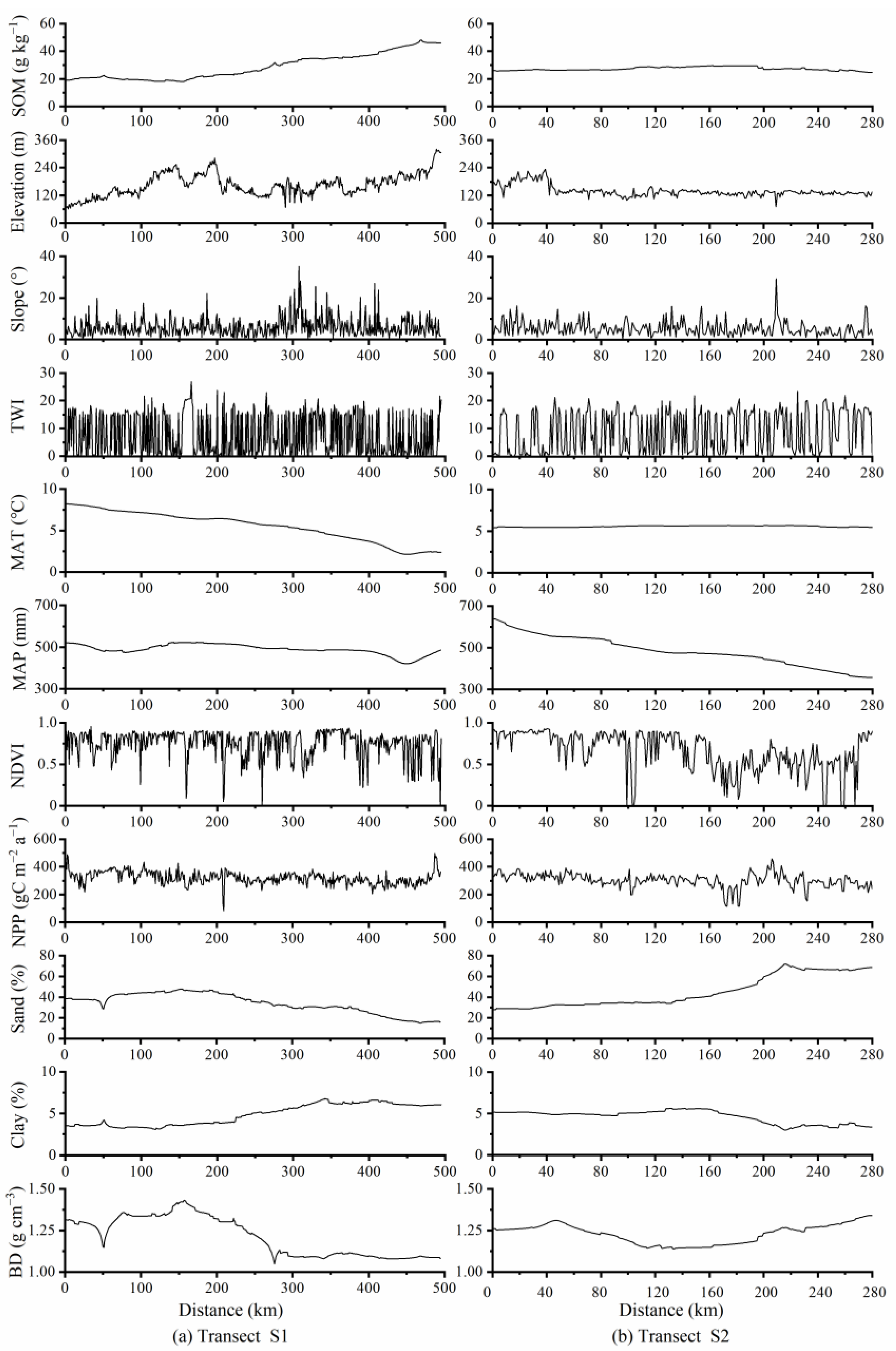
3.1. Characteristics of SOM and Environmental Factors

The mean values of SOM along the two transects were similar (

Table 1. Statistical characteristics of soil organic matter (SOM) and environmental factors along the S1 and S2 transects.

Transect		SOM (g kg−1)	Elevation (m)	Slope (°)	TWI	MAT (°C)	MAP (mm)	NDVI	NPP (gC m−2 a−1)	Sand (%)	Clay (%)	BD (g cm−3)
S1	Mean	28.84	164.48	5.88	7.55	5.50	489.27	0.75	320.03	34.17	4.85	1.21
	Minmum	18.02	61.00	0.00	0.01	2.13	420.70	0.00	82.40	15.07	3.08	1.05
	Maxmum	48.03	320.00	35.24	26.86	8.22	522.54	0.95	496.60	47.67	6.77	1.43
	Deviation	9.22	49.02	4.65	7.52	1.79	24.65	0.17	54.11	9.65	1.24	0.12
	CV (%)	31.98	29.80	78.97	99.63	32.59	5.04	22.58	14.44	28.25	25.47	9.67
S2	Mean	27.22	138.95	5.36	8.75	5.55	482.50	0.65	303.41	45.11	4.60	1.23
	Minmum	24.58	72.00	0.00	0.13	5.41	356.03	0.00	114.40	27.97	2.99	1.14
	Maxmum	29.75	233.00	29.35	23.33	5.67	639.25	0.93	457.40	72.05	5.64	1.34
	Deviation	1.30	24.97	3.65	7.69	0.08	71.19	0.24	49.65	14.99	0.76	0.06
	CV (%)	4.76	17.97	68.05	87.83	1.50	14.75	36.49	16.36	33.23	16.53	4.70

). However, the SOM variation along the S1 transect (CV = 31.98%) was more intense than that along the S2 transect (CV = 4.76%). Along the S1 transect, a general increasing trend of SOM was observed from southwest to northeast (Figure 3). Along the S2 transect, SOM was stably kept at 27 g kg⁻¹, and the change in SOM was less than 5 g kg⁻¹. Similarly, the mean and variability of elevation along the S1 transect were slightly greater than those along the S2 transect. Elevation increased at the beginning of the S1 transect, then decreased, and finally increased again from southwest to northeast. The elevation along the S2 transect initially decreased and then remained stable. Slope, TWI, NDVI, and NPP oscillated strongly along both transects. The NDVI and NPP values were higher along the S1 transect compared to the S2 transect because of its higher elevation and forest cover.

The mean MAT and MAP values were approximately equal along the two transects. However, the spatial trend of MAT along both transects was opposite to the spatial trend of MAP. Along the S1 transect from southwest to northeast, the MAT decreased from the transect to approximately 450 km MAT and then kept stable. A similar trend was observed for MAP from southwest to northeast along the S1 transect. However, the decreasing trend was stopped at around 480 mm. In contrast, MAT stabilized around 5.5 °C along the entire S2 transect, whereas MAP showed a decreasing trend from southeast to northwest with a reduction by nearly 40 mm per 40 km from the transect.

The mean sand content along the S1 transect was smaller than that of the S2 transect. Along the S1 transect, the sand content decreased sharply from 0–50 km, increased slightly from 50–150 km, and decreased gradually from 150 km to the end of the S1 transect. For the S2 transect, the sand content gradually increased from 0–250 km and then decreased until the end. The clay content showed an opposite variation trend compared to the sand along the S1 and S2 transects. The BD decreased dramatically at the beginning of the S1 transect and followed by an increase, then decreased again and finally remained stable at the end. Along the S2 transect, BD increased at the beginning of the transect and then decreased, and then increased again. Along the S1 transect, the variation of BD was greater than that of the S2 transect.

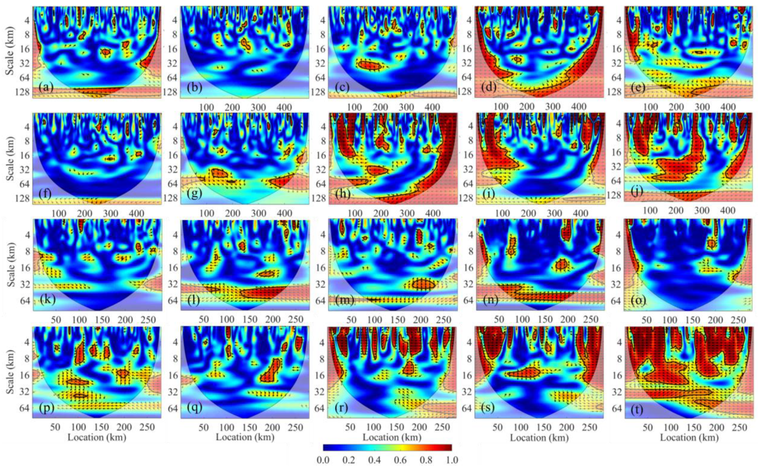
3.2. Single Environmental Factor Explaining SOM Variability

Figure 4 shows the BWC between the SOM and single environmental factor along both transects. There is a strong coherence in the red area. The area surrounded by the black thick contours is at the 95% significant level, and the pale area outside the thin black line is the cone of influence, where the edge effects influence the explanation. The arrows pointing to the right and left indicate positive and negative correlations, respectively. The overall correlation between SOM and elevation or clay was positive for both transects. Conversely, the correlation between SOM and MAT, NDVI, sand, or BD was negative.

Table 2. Wavelet coherence between soil organic matter (SOM) and single environmental factors along the S1 and S2 transect.

Transect	Factor	Small Scale (<32 km)		Medium Scale (32–64 km)		Large Scale (>64 km)		All Scales
		AWC	PASC(%)	AWC	PASC(%)	AWC	PASC(%)	AWC	PASC(%)
S1	Elevation	0.33	10.43	0.33	10.62	0.58	31.08	0.39	14.96
	Slope	0.25	3.12	0.22	0.00	0.27	0.00	0.25	1.96
	TWI	0.27	4.40	0.20	6.43	0.15	0.00	0.23	3.76
	MAT	0.39	20.24	0.60	49.23	0.75	70.65	0.50	35.69
	MAP	0.36	11.77	0.34	0.00	0.68	31.94	0.43	14.36
	NDVI	0.24	1.84	0.18	0.00	0.28	0.00	0.24	1.16
	NPP	0.27	2.91	0.57	29.43	0.43	5.28	0.35	7.51
	Sand	0.53	32.17	0.55	40.39	0.70	63.76	0.57	40.32
	Clay	0.48	31.17	0.41	20.56	0.42	5.01	0.46	23.84
	BD	0.55	36.07	0.58	33.74	0.61	46.25	0.57	37.93
S2	Elevation	0.28	3.86	0.28	3.01	0.15	0.00	0.27	3.31
	Slope	0.27	1.98	0.70	45.60	0.22	0.00	0.34	9.47
	TWI	0.29	3.77	0.31	6.13	0.21	0.00	0.28	3.80
	MAT	0.29	11.12	0.64	55.98	0.22	0.00	0.34	17.89
	MAP	0.29	13.83	0.25	0.71	0.34	0.00	0.29	10.09
	NDVI	0.35	7.98	0.49	1.40	0.22	0.00	0.36	6.00
	NPP	0.27	5.41	0.30	0.00	0.16	0.00	0.27	3.90
	Sand	0.49	28.47	0.39	8.63	0.46	8.83	0.47	22.95
	Clay	0.50	31.72	0.39	1.64	0.22	0.00	0.45	23.15
	BD	0.72	58.77	0.58	37.11	0.32	12.30	0.66	50.16

indicates the AWC and PASC of the BWC between the SOM and individual factor along both transects. Along the S1 transect, edaphic factors dominated SOM variability at all scales. Sand was the strongest factor controlling the variations in SOM, as indicated by the largest AWC (0.57) and PASC (40.32%) at all scales. There was a strong negative correlation between sand and SOM at all scales after 400 km along the transect. The other two edaphic factors, clay and BD, also displayed strong control on SOM variability with AWC values of 0.57 and 0.46, respectively.

Climatic was the second most critical factor, with relatively high AWC values for MAT (0.50) and MAP (0.43) at all scales. MAT was the major factor to explain the SOM variability at medium and large scales, with the AWC of 0.75 and 0.60 (Table 2). Topographic and vegetation factors displayed weak control over SOM variability.

For the S2 transect, edaphic factors showed the strongest effect in interpreting SOM variability at all scales. In particular, BD was the principal single factor to explain SOM variability at all scales with the maximum values of AWC (0.66) and PASC (50.16%) (Figure 4t). It showed dominance in explaining SOM variations at a small scale (AWC = 0.70 and PASC = 58.77%). Sand and clay also displayed a strong control on SOM variations at all scales with AWC values of 0.47 and 0.45. The significant coherence areas of BD broadly included those of sand and clay (Figure 4r–t). Among the topographic factors, slope had the largest AWC value (0.70) and a relatively higher PASC value (45.60%), indicating its critical role in the explanation of SOM variability at medium scale. Compared to slope, elevation and TWI showed weaker control on SOM variations. For climatic factors, MAT and MAP had high AWC (0.64 and 0.34) at medium and large scales, respectively. Similar to the case of S1 transect, the vegetation factor had a weaker control on SOM variability.

The above results indicate that a single environmental factor can only dominate SOM variations at specific scales and locations, but not for all scales and locations (Figure 4a–t). This implies that environmental factors cannot independently dominate the SOM variations.

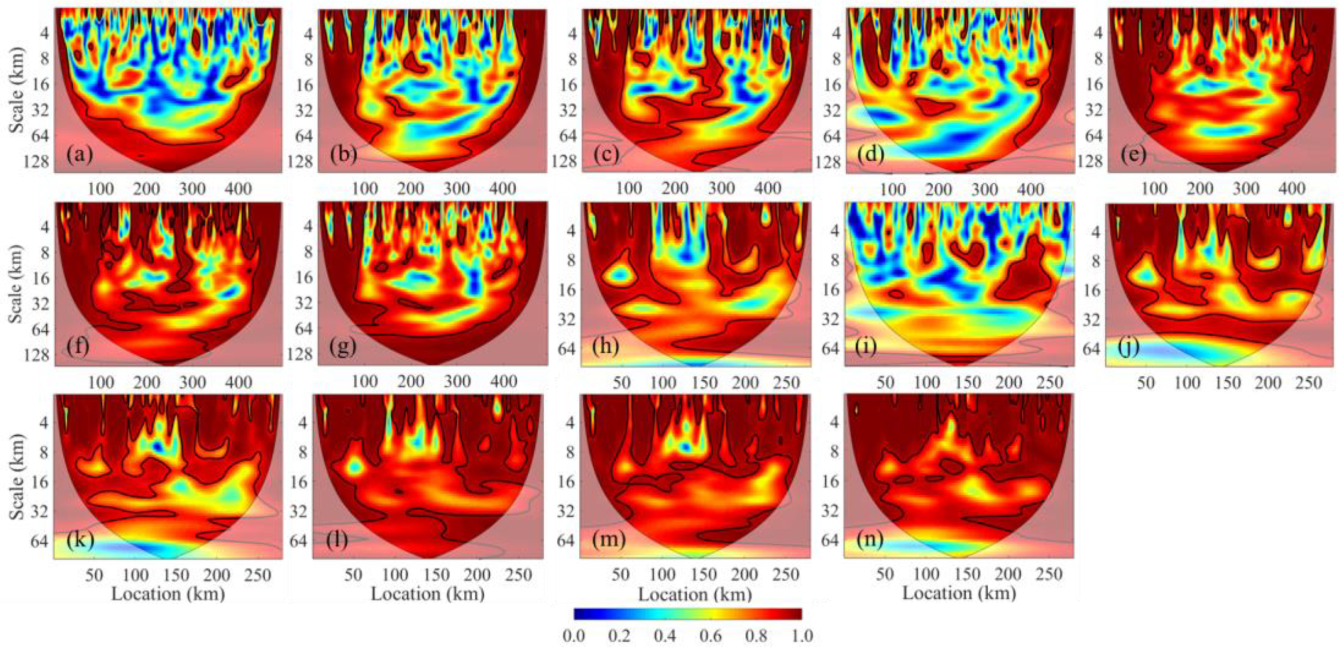
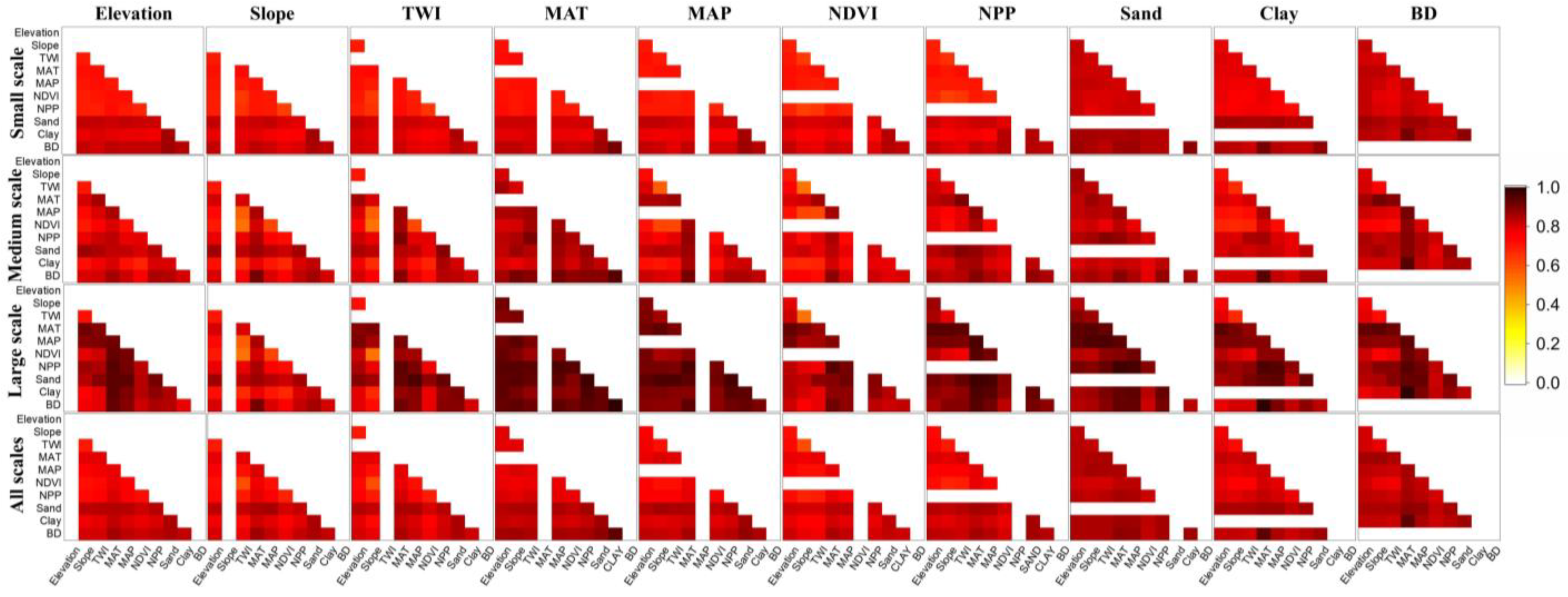
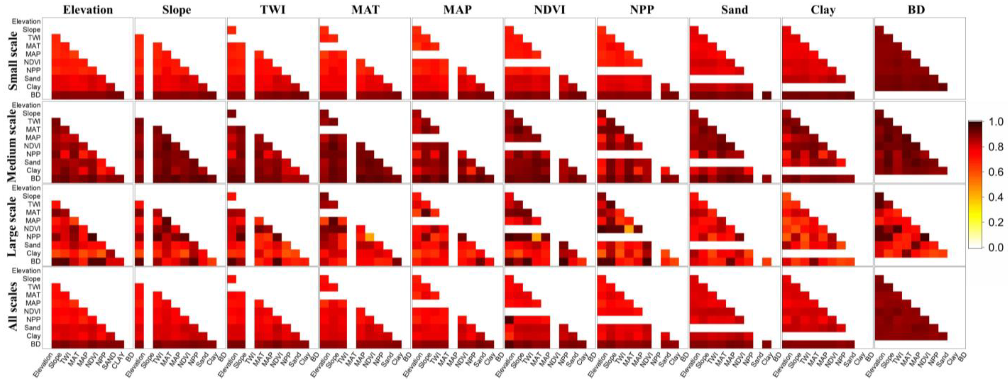
3.3. Multiple Environmental Factors Explaining SOM Variability

MWC between SOM and the combinations of typical multiple environmental factors are shown in Figure 5 and

Table 3. Wavelet coherence between soil organic matter (SOM) and single environmental factors along the S1 and S2 transect.

Transect	Factor	Small Scale (<32 km)		Medium Scale (32–64 km)		Large Scale (>64 km)		All Scales
		AWC	PASC(%)	AWC	PASC(%)	AWC	PASC(%)	AWC	PASC(%)
S1	MAT + NPP	0.56	17.85	0.79	54.16	0.93	94.07	0.68	40.05
	MAT + Sand	0.71	35.06	0.76	48.05	0.88	69.48	0.75	44.56
	MAT+BD	0.74	40.15	0.83	57.64	0.88	55.67	0.78	46.23
	NDVI + Sand	0.78	25.98	0.75	23.57	0.83	27.36	0.76	25.91
	MAT + Sand + CLAY	0.85	43.22	0.82	39.07	0.93	62.91	0.86	46.87
	MAT + Sand + BD	0.87	46.92	0.89	50.86	0.94	54.76	0.89	49.23
	NPP + MAT + Sand	0.81	32.67	0.87	48.91	0.98	93.38	0.86	48.40
S2	MAP+BD	0.82	50.82	0.88	57.77	0.63	9.95	0.81	47.84
	NDVI+NPP	0.54	7.33	0.61	0.06	0.80	12.35	0.58	6.56
	Sand + BD	0.85	57.84	0.81	59.40	0.59	3.32	0.82	52.51
	Clay + BD	0.87	62.05	0.82	40.12	0.53	1.89	0.82	51.99
	MAP + Sand + BD	0.90	51.14	0.95	59.64	0.93	22.35	0.92	49.68
	MAP + Clay + BD	0.91	53.72	0.91	45.18	0.74	3.06	0.89	47.00
	Sand + Clay + BD	0.93	62.37	0.88	40.95	0.64	0.00	0.89	52.17

. The AWC between SOM and the two or three-factor combinations is shown in Figure 6, Figure 7 and Figure 8. The AWC between SOM and the combination of multiple environmental factors along both transects was always greater than that of a single factor, confirming that the SOM was due to the coupling effect of environmental factors. The AWC generally increased with the addition of environmental factors.

The combination of climatic and edaphic factors improved the performance at all scales along the S1 transect for the cases of two-factor combinations. The combination of MAT and BD showed the best interpretation of SOM at all scales, as shown by the largest AWC (0.78). Additionally, it dominated the SOM variability at the medium scale (AWC = 0.88). At the large scale, the combination of climatic factors and other factors indicated the best explanation of SOM. In particular, the combination of MAT and NPP was the largest AWC (0.93). Additionally, the combination of edaphic factors and other factors showed the best explanation of SOM at a small scale. Particularly, the combination of NDVI and sand displayed the strongest control on SOM variability with the largest AWC (0.78).

Along the S2 transect, the performance of the combination of two edaphic factors were greatly improved at all scales. The combination of BD and sand or clay indicated the largest AWC (both 0.82). The best factors to explain SOM variability were different at various scales. Specifically, the combination of NDVI and NPP, MAP and BD, clay and BD, had the best explanation for SOM at large, medium, and small scales, separately.

Among the three-factors cases, the combination of climatic and edaphic factors had the best explanation for the variations in SOM, due to the dominance of the combined control of climatic factors at medium and large scales and edaphic factors at all scales. The combination of MAT, sand, and BD showed the largest AWC (0.89) along the S1 transect at all scales. Along the S2 transect, the combination of MAP, sand, and BD had the best explanation of SOM at all scales with the largest AWC (0.92), which was due to the combination of BD and other factors that enhanced the explanation of SOM variability at each scale.

4. Discussion

4.1. Anisotropy and Scale-Location Specific Factors Explaining SOM

The results show that the scale and location-specific variations in SOM and environmental factors were direction-specific. Edaphic factors were important in explaining SOM variations along both transects. This is consistent with the findings that edaphic factors displayed a strong ability to explain SOM variations in dryland farming regions [32]. The strongest single factor explaining SOM variability was different between the two dominant directions. Sand provided the best explanation for SOM variations along the major direction due to the significant negative correlation between sand and SOM from 400 km to the end of the transect. Sand is relatively inert and well drained, leading to higher SOM oxidation and counting against the retention and protection of SOM [33]. The most influential single factor explaining SOM variations along the minor direction was the BD. The BD reflects the conditions of soil porosity and compaction, and it is closely bound up with the water and solute transport, soil respiration, and root growth, which greatly influences the dynamic processes of SOM [34].

Climatic factors were considered to be the main drivers of SOM distribution over a large scale [35,36]. With decreasing temperature and increasing precipitation, the decomposition rate usually decreases, leading to the accumulation of SOM. Our study indicates that climatic factors show a strong control at large scale along the major direction whereas the control was absent along the minor direction. This might be because latitudinal variations were not enough to influence the distribution of temperature along the minor direction. However, the underlying causes need to be explored more.

It is widely accepted that topographic factors play a key role in influencing soil properties [37,38]. Topographic factors indirectly control SOM by altering the microclimate that influences the decomposition of SOM [39]. However, in the present study, topographic factors were not significantly controlled at all scales. The reason for this is that the topography in Songliao Plain is relatively flat and the sampling points were mainly distributed in dryland where slopes are less than 5° [32].

Vegetation factors did not exhibit a distinct correlation with SOM variations. This may be due to the long history of cultivation and intensive agricultural practices in the study area [40]. Vegetation production is highly dependent on the agronomic management, such as tillage and fertilization practice. The effect of vegetation factors conditions on SOM was not as pronounced as anthropogenic factors. However, it is worthwhile mentioning that the combination of vegetation factors and other factors showed a strong ability to interpret the variations in SOM. This may be due to the significant coherent area between the SOM and vegetation factors supplementing the low coherent area between SOM and other factors at various scales.

4.2. Can More Factors Be Included to Better Explain SOM Variability?

As shown previously, an increase in the number of factors may lead to an increase in AWC. Hu and Si reported that AWC could increase with the number of factors, but PASC does not [20]. AWC and PASC for combinations of four or more factors were also calculated. For example, when clay was added to the combination of MAT, sand, and BD (the best three-factor combination) along the major direction, AWC increased from 0.89 to 0.94, while PASC decreased from 49.23% to 47.06%. This is because most areas with significant coherence between SOM and MAT are superposed with those of SOM and BD. The increment of AWC gradually shrank when the factors increase to four or more. However, the change in PASC was <5%, which was not statistically significant. Thus, in our study, the combination of two factors is adequate to explain SOM variability along the major direction, whereas a single factor (i.e., BD) is sufficient along the minor direction. Previous studies have typically included too many variables to explain SOM variability [41,42,43]. This may be redundant and even reduce the ability to explain SOM variability [44], due to ignoring the anisotropy and scale-location dependence relationship between SOM and environmental factors.

5. Conclusions

In this study, the anisotropy and scale-location dependence relationship between SOM and multiple environmental factors was explored in dryland farming regions of Songliao Plain, China by multiple wavelet coherence and anisotropic analysis. Two dominant directions of SOM spatial distribution were found. Specifically, the major direction along which SOM varied the most significantly was 56° east by north, and the minor direction was perpendicular to the major direction. At all scales, edaphic factors were important in controlling SOM variation. The strongest single factor explaining SOM variations was different between two dominant directions, with sand along the major direction and BD along the minor direction. The combination of MAT and BD performed best in explaining SOM variability along the major direction, with a significant increase in both AWC and PASC. Our work shows that the two-factor combination is sufficient to explain the SOM variations along the major direction, whereas a single factor is adequate along the minor direction. Therefore, the SOM variations can be better explained in an efficient way with few variables after considering the anisotropy and scale-location dependence relationship between SOM and environmental factors.

References

1. Tiessen, H.; Cuevas, E.; Chacon, P. The role of soil organic matter in sustaining soil fertility. Nature 1994, 371, 783–785. [Google Scholar] [CrossRef]
2. Davidson, E.A.; Janssens, I.A. Temperature sensitivity of soil carbon decomposition and feedbacks to climate change. Nature 2006, 440, 165–173. [Google Scholar] [CrossRef] [PubMed] [Green Version]
3. Biswas, A. Scale–location specific soil spatial variability: A comparison of continuous wavelet transform and Hilbert-Huang transform. Catena 2018, 160, 24–31. [Google Scholar] [CrossRef]
4. Bonfatti, B.R.; Hartemink, A.E.; Giasson, E.; Tornquist, G.C.; Adhikari, K. Digital mapping of soil carbon in a viticultural region of southern brazil. Geoderma 2016, 261, 204–221. [Google Scholar] [CrossRef]
5. Guan, J.H.; Deng, L.; Zhang, J.G.; He, Q.Y.; Shi, W.Y.; Li, G.; Du, S. Soil organic carbon density and its driving factors in forest ecosystems across a northwestern province in China. Geoderma 2019, 352, 1–12. [Google Scholar] [CrossRef]
6. Mishra, U.; Hugelius, G.; Shelef, E.; Yang, Y.; Strauss, J.; Lupachev, A.; Harden, J.M.; Jastrow, J.D.; Ping, C.L.; Riley, W.J.; et al. Spatial heterogeneity and environmental predictors of permafrost region soil organic carbon stocks. Sci. Adv. 2021, 7, 5236. [Google Scholar] [CrossRef]
7. Zeleke, T.B.; Si, B.C. Characterizing scale-dependent spatial relationships between soil properties using multifractal techniques. Geoderma 2006, 134, 440–452. [Google Scholar] [CrossRef]
8. Webster, R. Spectral analysis of gilgai soil. Aust. J. Soil Res. 1977, 15, 191–204. [Google Scholar] [CrossRef]
9. Guo, Y.D.; Zhao, R.Y.; Zeng, Y.N.; Shi, Z.; Zhou, Q. Identifying scale-specific controls of soil organic matter distribution in mountain areas using anisotropy analysis and discrete wavelet transform. Catena 2018, 160, 1–9. [Google Scholar] [CrossRef]
10. Zhu, H.F.; Hu, W.; Jing, Y.D.; Cao, Y.; Bi, R.T.; Yang, W.D. Soil organic carbon prediction based on scale-specific relationships with environmental factors by discrete wavelet transform. Geoderma 2018, 330, 9–18. [Google Scholar] [CrossRef]
11. Biswas, A.; Cresswell, H.P.; Viscarra Rossel, R.A.; Si, B.C. Separating scale-specific spatial variability in two dimensions using bi-dimensional empirical mode decomposition. Soil Sci. Soc. Am. J. 2013, 77, 1991. [Google Scholar] [CrossRef]
12. Zhou, Y.; Chen, S.C.; Zhu, A.X.; Hu, B.F.; Shi, Z.; Li, Y. Revealing the scale- and location-specific controlling factors of soil organic carbon in Tibet. Geoderma 2021, 382, 114713. [Google Scholar] [CrossRef]
13. Biswas, A.; Cresswell, H.P.; Rossel, R.V.; Si, B.C. Characterizing scale- and location-specific variation in non-linear soil systems using the wavelet transform. Eur. J. Soil Sci. 2013, 64, 706–715. [Google Scholar] [CrossRef]
14. Bahri, H.; Raclot, D.; Barbouchi, M.; Lagacherie, P.; Annabi, M. Mapping soil organic carbon stocks in Tunisian topsoils. Geoderma Reg. 2022, 30, e00561. [Google Scholar] [CrossRef]
15. Koopman, L.H. The Spectral Analysis of Time Series; Academic Press: Cambridge, MA, USA, 1974; pp. 119–164. [Google Scholar]
16. Si, B.C. Spatial scaling analyses of soil physical properties: A review of spectral and wavelet methods. Vadose Zone J. 2008, 7, 547. [Google Scholar] [CrossRef] [Green Version]
17. Fleureau, J.; Kachenoura, A.; Albera, L.; Nunes, J.; Senhadji, L. Multivariate empirical mode decomposition and application to multichannel filtering. Signal Process. 2011, 91, 2783–2792. [Google Scholar] [CrossRef] [Green Version]
18. Zhu, H.F.; Cao, Y.; Jing, Y.D.; Liu, G.; Bi, R.; Yang, W.D. Multi-scale spatial relationships between soil total nitrogen and influencing factors in a basin landscape based on multivariate empirical mode decomposition. J. Arid Land 2019, 11, 385–399. [Google Scholar] [CrossRef] [Green Version]
19. Zhu, X.C.; Liang, Y.; Tian, Z.Y.; Wang, X. Analysis of scale-specific factors controlling soil erodibility in southeastern China using multivariate empirical mode decomposition. Catena 2021, 199, 105131. [Google Scholar] [CrossRef]
20. Hu, W.; Si, B.C. Technical note: Multiple wavelet coherence for untangling scale specific and localized multivariate relationships in geosciences. Hydrol. Earth Syst. Sci. 2016, 20, 3183–3191. [Google Scholar] [CrossRef] [Green Version]
21. Agarwal, A.; Marwan, N.; Rathinasamy, M.; Merz, B.; Kurths, J. Multi-scale event synchronization analysis for unravelling climate processes: A wavelet-based approach. Nonlin. Process. Geophys. 2017, 24, 599–611. [Google Scholar] [CrossRef]
22. Centeno, L.N.; Hu, W.; Timm, L.C.; She, D.; da Silva Ferreira, A.; Barros, W.S.; Beskow, S.; Caldeira, T.L. Dominant control of macroporosity on saturated soil hydraulic conductivity at multiple scales and locations revealed by wavelet analyses. J. Soil Sci. Plant Nutr. 2020, 20, 1686–1702. [Google Scholar] [CrossRef]
23. Trangmar, B.B.; Yost, R.S.; Uehara, G. Application of geostatistics to spatial studies of soil properties. Adv. Agron. 1985, 38, 45–94. [Google Scholar] [CrossRef]
24. Burgess, T.M.; Webster, R. Optimal interpolation and isarithmic mapping of soil properties. I. The semivariogram and punctual kriging. Eur. J. Soil Sci. 2019, 31, 315–331. [Google Scholar] [CrossRef]
25. Biswas, A.; Cresswell, H.P.; Viscarra Rossel, R.A.; Si, B.C. Curvelet transform to study scale-dependent anisotropic soil spatial variation. Geoderma 2014, 213, 589–599. [Google Scholar] [CrossRef]
26. Simon, G. An angular version of spatial correlations with exact significance tests. Geogr. Anal. 1997, 29, 267–278. [Google Scholar] [CrossRef]
27. Zhao, R.; Biswas, A.; Zhou, Y.; Zhou, Y.; Shi, Z.; Li, H. Identifying localized and scale-specific multivariate controls of soil organic matter variations using multiple wavelet coherence. Sci. Total Environ. 2018, 643, 548–558. [Google Scholar] [CrossRef]
28. Zhu, H.F.; Hu, W.; Ding, H.X.; Lv, C.J.; Bi, R.T. Scale- and location-specific multivariate controls of topsoil organic carbon density depend on landform heterogeneity. Catena 2021, 207, 105695. [Google Scholar] [CrossRef]
29. Tian, H.W.; Zhang, J.H.; Zhu, L.Q.; Liu, M.; Shi, J.Q.; Li, G.D. Revealing the scale- and location-specific relationship between soil organic carbon and environmental factors in China’s north-south transition zone. Geoderma 2022, 409, 115600. [Google Scholar] [CrossRef]
30. Huang, J.Y.; Shi, Z.; Biswas, A. Characterizing anisotropic scale-specific variations in soil salinity from a reclaimed marshland in China. Catena 2015, 131, 64–73. [Google Scholar] [CrossRef]
31. Grinsted, A.; Moore, J.C.; Jevrejeva, S. Application of the cross wavelet transform and wavelet coherence to geophysical time series. Nonlin. Process. Geophys. 2004, 11, 561–566. [Google Scholar] [CrossRef]
32. Zhuo, Z.Q.; Chen, Q.Q.; Zhang, X.L.; Chen, S.C.; Gou, Y.X.; Sun, Z.X.; Huang, Y.F.; Shi, Z. Soil organic carbon storage, distribution, and influencing factors at different depths in the dryland farming regions of Northeast and North China. Catena 2022, 210, 105934. [Google Scholar] [CrossRef]
33. Augustin, C.; Cihacek, L.J. Relationships between soil carbon and soil texture in the Northern Great Plains. Soil Sci. 2007, 181, 386–392. [Google Scholar] [CrossRef]
34. Liu, Z.P.; Shao, M.A.; Wang, Y.Q. Estimating soil organic carbon across a large-scale region: A state-space modeling approach. Soil Sci. 2012, 177, 607–618. [Google Scholar] [CrossRef]
35. Heimann, M.; Reichstein, M. Terrestrial ecosystem carbon dynamics and climate feedbacks. Nature 2008, 451, 289–292. [Google Scholar] [CrossRef] [PubMed] [Green Version]
36. Carey, C.J.; Weverka, J.; Digaudio, R.; Gardali, T.; Porzig, E.L. Exploring variability in rangeland soil organic carbon stocks across California (USA) using a voluntary monitoring network. Geoderma Reg. 2020, 22. [Google Scholar] [CrossRef]
37. Grimm, R.; Behrens, T.; Marker, M.; Elsenbeer, H. Soil organic carbon concentrations and stocks on Barro Colorado Island-digital soil mapping using random forests analysis. Geoderma 2008, 146, 102–113. [Google Scholar] [CrossRef]
38. Zhang, S.W.; Huang, Y.F.; Shen, C.Y.; Ye, H.C.; Du, Y.C. Spatial prediction of soil organic matter using terrain indices and categorical variables as auxiliary information. Geoderma 2012, 171, 35–43. [Google Scholar] [CrossRef]
39. Chen, L.; He, Z.; Du, J.; Yang, J.; Zhu, X. Patterns and environmental controls of soil organic carbon and total nitrogen in alpine ecosystems of northwestern China. Catena 2016, 137, 37–43. [Google Scholar] [CrossRef]
40. Zhou, Y.; Biswas, A.; Ma, Z.; Lu, Y.; Chen, Q.; Shi, Z. Revealing the scale-specific controls of soil organic matter at large scale in Northeast and North China Plain. Geoderma 2018, 271, 71–79. [Google Scholar] [CrossRef]
41. Schillaci, C.; Acutis, M.; Lombardo, L.; Lipani, A.; Fantappie, M.; Marker, M.; Saia, S. Spatio-temporal topsoil organic carbon mapping of a semi-arid Mediterranean region: The role of land use, soil texture, topographic indices and the influence of remote sensing data to modelling. Sci. Total Environ. 2017, 601–602, 821–832. [Google Scholar] [CrossRef]
42. Wiesmeier, M.; Urbanski, L.; Hobley, E.; Lang, B.; von Lützow, M.; Marin-Spiotta, E.; van Wesemael, B.; Rabot, E.; Ließ, M.; Garcia-Franco, N.; et al. Soil organic carbon storage as a key function of soils–a review of drivers and indicators at various scales. Geoderma 2019, 333, 149–162. [Google Scholar] [CrossRef]
43. Adhikari, K.; Mishra, U.; Owens, P.R.; Libohova, Z.; Wills, S.A.; Riley, W.J.; Hoffman, F.M.; Smith, D.R. Importance and strength of environmental controllers of soil organic carbon changes with scale. Geoderma 2020, 375, 114472. [Google Scholar] [CrossRef]
44. Hu, W.; Si, B.C.; Biswas, A.; Chau, H.W. Temporally stable patterns but seasonal dependent controls of soil water content: Evidence from wavelet analyses. Hydrol. Process. 2017, 31, 3697–3707. [Google Scholar] [CrossRef]
Figure 1. The location of study area in Songliao Plain (a); the distribution of sampling points (b); and the main soil types (c).
Sustainability 14 12569 g001
Figure 2. The distribution of soil organic matter (SOM) across the study area and location of S1 and S2 transects.
Sustainability 14 12569 g002
Figure 3. Spatial distribution of soil organic matter (SOM) and environmental factors along the S1 and S2 transects.
Sustainability 14 12569 g003
Figure 4. Bivariate wavelet coherency between soil organic matter (SOM) and individual factor along the S1 and S2 transect. Arrows show the phase angles of the wavelet spectra. Thin solid lines demarcate the cones of influence and thick solid lines show the 95% significance levels. Note: (at) represent wavelet coherency spectra between Elevation, Slope, TWI, MAT, MAP, NDVI, NPP, Sand, Clay and BD along S1 and S2 transects, successively.
Sustainability 14 12569 g004
Figure 5. Multivariate wavelet coherency between soil organic matter (SOM) and typical multiple factors combinations (a) MAT and NPP, (b) MAT and Sand, (c) MAT and BD, (d) NDVI and Sand, (e) MAT, Sand, and Clay, (f) MAT, Sand, and BD, (g) NPP, MAT, and Sand along the S1 transect. Multivariate wavelet coherency between SOM and typical multiple factors combinations (h) MAP and BD, (i) NDVI and NPP, (j) Sand and BD, (k) Clay and BD, (l) MAP, Sand, and BD, (m) MAP, Clay, and BD, (n) Sand, Clay, and BD along the S2 transect.
Sustainability 14 12569 g005
Figure 6. Average wavelet coherence (AWC) between soil organic matter (SOM) and the combination of each two factors along the S1 and S2 transects. The small scale is <32 km, medium scale is between 32 and 64 km, and large scale is >64 km. All scales are indicated by the overall coherence.
Sustainability 14 12569 g006
Figure 7. Average wavelet coherence (AWC) between soil organic matter (SOM) and the combination of each three factors along the S1 transect. The small scale is <32 km, medium scale is between 32 and 64 km, and large scale is >64 km. All scales are indicated by the overall coherence.
Sustainability 14 12569 g007
Figure 8. Average wavelet coherence (AWC) between soil organic matter (SOM) and the combination of each three factors along the S2 transect. The small scale is <32 km, medium scale is between 32 and 64 km, and large scale is >64 km. All scales are indicated by the overall coherence.
Sustainability 14 12569 g008