Abstract
Wildfires are a major environmental issue that have an impact on land degradation. Remote sensing spectral indices provide valuable information for short-term mitigation and rehabilitation after wildfires. A study area in the Centre inland of Portugal occupied with Maritime pine and Eucalypts forests and affected by wildfires in 2003, 2017 and 2020 was used. The aims of the study were twofold: (1) to compute the Normalized Difference Vegetation Index (NDVI) and with forest inventory data derivate a Maritime pine production model, differentiate evergreen coniferous forests (e.g., Maritime pine), evergreen broadleaved forests (e.g., Eucalypts), and shrubland, and monitor vegetation and its post-fire recovery; and (2) to compute the Normalized Burn Ratio (NBR) difference between pre-fire and post-fire dates for burn severity levels assessment. The plots of a previous forest inventory were used to follow the NDVI values in 2007 and from 2020 to 2022. An aerial coverage in 2007 and the Sentinel-2 imagery in 2020–2022 were used. Linear models fitted maritime pine production with the transformed NDVI by age, showing a fitting efficiency of 60%. The stratification of cover types by stand development stage and fire occurrence was possible using the NDVI time curve, which also showed the impact of fire and of low precipitation. Cover types were ranked by decreasing NDVI values as follows: mature Eucalypts plantations, young Maritime pine regeneration, mature Maritime pine, young Eucalypts plantations, Strawberry tree shrubland, Eucalypts plantations post-fire, Maritime pine post-fire, tall shrubland, and short shrubland. Vegetation post-fire recovery was lower in higher burn severity level areas. Maritime pine areas have lost their natural regeneration capability due to the wildfires’ short cycles. Spectral indices were effective tools to differentiate cover types and assist in the evaluation of forest and shrubland conditions.
1. Introduction
In a wide range of world ecosystems, wildfires constitute a major environmental issue and, in some cases, are a significant cause of land degradation [1]. Wildfires are a problematic and recurrent issue in Mediterranean ecosystems, especially in countries such as Spain and Portugal [2,3,4]. They are a major disturbance factor for Mediterranean forests and play a critical role in the cycle of vegetation succession and ecosystem structure and function [5]. Currently, there is a growing concern about the ecological and socio-economic impacts of wildfires, particularly under a climate change context that implies an increase in the frequency and severity of wildfires in European countries in the future [6].
Remote sensing can provide valuable information about the type and status of the vegetation in a consistent way at different spatial and temporal scales [7]. Currently, a variety of remotely sensed imagery sources are available with different known spectral, spatial, radiometric and temporal resolutions increasing the choice and suitability for different purposes of vegetation mapping [8]. Furthermore, remotely sensed imagery can be processed and transformed to enhance the target phenomena under study [9,10].
One of the most common techniques of imagery enhancement is the computation of spectral indices [10]. These indices use the most sensitive spectral bands that allow highlighting a particular target (e.g., land cover and/or its change and temporal trend). Nowadays, the most popular spectral indices in use are the Normalized Difference Vegetation Index (NDVI) and the Normalized Burn Ratio (NBR), respectively, to monitor vegetation productivity [11,12,13,14,15,16] and to detect burned areas and their severity [2,3,4,9,17,18,19]. These indices have also been incorporated in time series analysis to systematically detect burned areas and monitor long-term vegetation recovery [9,20,21,22,23,24,25].
The NDVI measures vegetation greenness and is related to the structural properties of plants (e.g., leaf area index and green biomass) and properties of vegetation productivity (e.g., absorbed photosynthetic active radiation and foliar nitrogen). As NDVI is related to various vegetation properties, multiple explanations for a change in NDVI are possible. Nevertheless, the NDVI is being successfully used to assess post-fire effects such as vegetation regrowth. This is appropriate if a direct change in green vegetation cover is the main ecological process being measured [21,26].
Since accurate, reliable, and timely burn severity maps are critical for short-term mitigation and rehabilitation after wildfires [2,17,27], the difference in NBR between pre-and post-fire images (dNBR) is also being used to infer fire severity from remotely sensed data [26]. Thus, providing important information regarding the impact of fire on the environment and how it is distributed throughout the burned area [27]. It is known that highly severe fires can greatly impact the ecosystem attributes and processes, namely soil erosion and sedimentation, habitat fragmentation and availability, patterns of vegetation and community recovery, alien plant invasion and carbon dynamics [28].
Satellite observations also provide a global NDVI time series dataset that allows the quantification and attribution of ecosystem changes due to ecosystem dynamics and varying climate conditions [15,21]. Some applications of the NDVI time series have been the retrospective modeling of forest productivity over larger areas regarding the maximum growing season NDVI [15] and the differentiation of forestland types, such as evergreen, deciduous, and mixed forests, by its characteristic NDVI time curves throughout the annual growing season [22]. Indeed, in the past years, NDVI time-series imagery has been widely used to monitor evergreen forests on a large scale. But when using low spatial resolution imagery to study large areas and/or low complexity landscapes, the mixed pixel problem should be considered when extracting land cover types [23].
Vegetation types can be differentiated as the NDVI annual mean or peak provides an integrated view of photosynthetic activity, the seasonal NDVI amplitude infers the composition of evergreen and deciduous vegetation and the length of the NDVI growing season can be related to phenological change. Regarding the occurrence of negative NDVI trends (“browning”), they are usually associated with fire activity, increasing water vapor pressure deficit or to cooling spring temperatures [15,21]. In that view, an NDVI-CV method is a methodological approach that was successfully applied to differentiate various types of vegetation. The method is based on the analysis of the NDVI time curve throughout the annual growing cycle by combining the annual minimum NDVI (NDVIann-min) with the observed coefficient of variation (CV) and so considering all the phenological critical phases to differentiate the cover types (e.g., evergreen trees, deciduous trees, mixed trees, farmland, and fallow land) [23].
For instance, when comparing the NDVI values of evergreen forests with deciduous forests throughout the year, the latter shows a lower NDVI before the green up. It increases rapidly from green up to maturity, stays higher from maturity to senescence and then gets lower again after dormancy. Conversely, evergreen forest NDVI values throughout the year are frequently high, with small-scale fluctuation. As might be expected, mixed forests combine the characteristics of both deciduous forests and evergreen forests: intermediate NDVI values before the green up and after dormancy and higher NDVI values from maturity to senescence but with a fluctuation range [22].
In Portugal, according to the National Forest Inventory (NFI) data, although Maritime pine (Pinus pinaster Aiton) was the most widespread species until 2005, the Eucalypts (mainly, Eucalyptus globulus Labill.) are presently the most abundant species (26%; 811,943 ha) followed by Cork oak (Quercus suber L.; 23%; 736,775 ha), Maritime pine (23%; 714,445 ha), and Holm oak (Quercus rotundifolia Lam.; 11%; 331,179 ha) [29]. Maritime pine is a native pioneer evergreen coniferous species mainly established by natural regeneration. In contrast, Eucalypts is an exotic evergreen broadleaved species installed by plantation. Maritime pine and Eucalypts forests provide most of the wood harvested in Portugal, used mainly as raw materials for the wood-based industry. In the last decades, the Maritime pine area has been decreasing mainly due to forest fires. Most of the species’ burned area has been converted into shrubland, pastures, and Eucalyptus plantations [29].
Moreover, both Maritime pine and Eucalypts forests have a concurrent geographical distribution in Portugal, so it is important to apply methodologies that may allow the differentiation of these two types of forests. Indeed, the NDVI-CV method has proved to be effective in extracting evergreen trees from other types of vegetation. As evergreen tree growth characteristics remain nearly unchanged during the phenological cycle, the NDVIann-min is the optimal moment to separate them from other vegetation types [23]. However, to our best knowledge, this method has not yet been essayed to differentiate evergreen coniferous forests (e.g., Maritime pine) from evergreen broadleaved forests (e.g., Eucalypts).
Therefore, this study’s research hypotheses were that the use of remotely sensed spectral indices would be effective: (1) to model Maritime pine production (wood and biomass) using the NDVI as the explanatory variable; (2) to differentiate evergreen coniferous forests (e.g., Maritime pine), evergreen broadleaved forests (e.g., Eucalypts), and shrubland by their NDVI time curve patterns; and (3) to monitor vegetation disturbances such as fire events and/or stress by weather conditions variations using the NDVI and the NBR.
Thus, the aims of this study were twofold: (1) to compute the NDVI and use forest inventory data to derivate a Maritime pine production model, differentiate evergreen coniferous forests (e.g., Maritime pine), evergreen broadleaved forests (e.g., Eucalypts), and shrubland, and monitor vegetation and its post-fire recovery; and (2) to compute the NBR difference of pre-fire and post-fire dates for burn severity levels assessment.
To that end, it was selected a study area in the Centre inland of Portugal mainly occupied by evergreen forests (Maritime pine naturally regenerated forests and Eucalypts plantations) and affected by wildfires in 2003, 2017 and 2020. The inventory data collected in 2007 and the NDVI computed from the aerial coverage of the same year were used for modeling purposes. After, the inventory plots were used to follow cover types change from 2007 to 2020 due to the occurrence of the wildfires. The Sentinel-2 imagery was used to compute the NDVI for 2020–2022 and the NBR pre and post 2000 wildfire dates. Plots’ NDVI values in 2007 and 2020 were used to explore cover types. The NDVI time curve throughout the 2020 growing season was used to differentiate the cover types. Regarding the last wildfire in 2000, the NBR was used to assess its severity and the NDVI to monitor the post-fire effects on vegetation and its recovery until the present year of 2022. The burn severity map for the 2020 wildfire was used to explain plots’ NDVI values post-fire and vegetation recovery. Climatological data was also used to explain other plots’ NDVI anomalies.
2. Materials and Methods
2.1. Study Area
The study area is a locality in the Centre inland of Portugal (Figure 1a) with 3100 ha of area. This study area, the locality of Sarnadas de S. Simão (6.04734° W, 6.11400° E, 44.19665° S, 44.28486° N), has suffered significant changes in its forest cover throughout the last decades. According to the Portuguese land cover/land use official maps (COS—Carta de Ocupação do Solo) [30], in 1995, the study area was mainly occupied by Maritime pine forest (Figure 1b). In 2007, due to the 2003 wildfire (Figure 2b), the Maritime pine forest decreased substantially (Figure 1c). After a decade, in 2017, another severe wildfire (Figure 2c) was the vector for the continuing decrease of Maritime pine forests and the increase of Eucalypts plantations (Figure 1d).
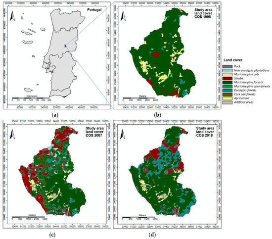
Figure 1.
Study area—locality of Sarnadas de S. Simão (Portugal): (a) Geographic location (6.04734° W, 6.11400° E, 44.19665° S, 44.28486° N); (b) land cover in 1995 (COS 1995); (c) land cover in 2007 (COS 2007); and (d) land cover in 2018 (COS 2018) [30].
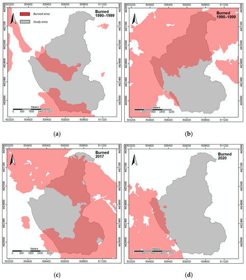
Figure 2.
Study area—locality of Sarnadas de S. Simão (Portugal)—burned area (1990–2020): (a) 1990–1999; (b) 2000–2008; (c) 2017; and (d) 2020 [31].
According to the Portuguese burned areas’ official maps [31], between 1990 and 1999 (Figure 2a), the study area was considerably burned. Later in 2003, a severe wildfire burned the study area’s northern zone (Figure 2b). Fourteen years later, in 2017, another severe wildfire burned the study area’s northern-east and southern-east zones extensively (Figure 2c). More recently, in 2020, a wildfire burned the study area’s western zone, a mountain area that integrates the Geopark of “Naturtejo da Meseta Meridional” belonging to the UNESCO World Geoparks (Figure 2d). As a result, currently, the only unburned area is located within an area set by the triangulation of the three settlements of this locality due to the efforts of firefighting to defend people and assets.
2.2. Data
2.2.1. Field Data—Forest Inventory (2007)
A forest inventory data performed in 2007 was used, wherein a systematic sampling supported by a geo-referenced 500 m spacing grid allowed to install 60 circular plots of 500 m2 [32].
Due to the wildfire in 2003 (Figure 2b), the northern zone was covered either by shrubland (13 plots) or by young naturally regenerated Maritime pine stands that were too small to be measured (18 plots) (Figure 1c). Differences in plot land cover in 2007 and the Portuguese official land cover map COS 2007 [30] are due to the minimum mapping unit used in that map (set as one ha) when compared with the plot area (500 m2) (Appendix A—Table A1).
The most representative species in shrubland areas were Cytisus sp., Cistus sp., and Erica sp., Arbutus unedo, Pterospartum tridentatum and Pteridium sp.
Maritime pine regeneration of around 1000 to 50,000 seedlings per ha was observed three-four years after the 2003 wildfire, although irregularly distributed over the plot area (ground cover ranging from 10 to 30 %). A better ground cover was verified in areas with shorter seedlings (Table 1) [32].

Table 1.
Forest inventory—summary statistics for Maritime pine natural regeneration (n = 18) [32].
Mature Maritime pine stands could only be found in the southern zone of this locality (25 plots; Figure 1b and Figure 2b). Eucalypts plantations were quite residual (one plot), but the species was also found in mixed dominant or dominated stands with Maritime pine (three plots). In each plot, the diameter at breast height (d) was measured for all trees larger than 5 cm. Tree total height (h) was measured in a subset of trees (sample trees) proportionally selected to the diameter class frequency and in dominant trees. The data collected allowed for an overall characterization of Maritime pine stands in 2007. The standard stand variables considered were the following: N, number of trees per hectare (trees ha−1); G, basal area per hectare (m2 ha−1); dg, quadratic mean diameter (cm); , mean height (m); ddom, dominant diameter (cm); hdom, dominant height (m); Fw, Wilson’s factor; t, stand age (year); Sh25, site productivity; and V, stand volume (m3 ha−1) (Table 2).
Table 2.
Forest inventory—summary statistics for Maritime pine stand variables (n = 25) [32].
Wilson’s factor (Fw) is a density index used to assess the stand stocking, and values of 0.11, 0.16, 0.20, 0.23 and 0.28 correspond, respectively, to the thinning grades A (natural mortality), C (light thinning), C/D, D and E (heavy thinning) [32].
Site productivity was assessed using a height index model (Sh25) that is defined as the expected tree height at the reference diameter of 25 cm [33]. The following was the correspondence between Sh25 and the mean annual increment of stand total volume at the rotation age of 45 years (MAI45): for Sh25 = 13 a MAI45 = 5 m3 ha–1 year–1, for Sh25 = 15 a MAI45 = 7 m3 ha–1 year–1 and for Sh25 = 17 a MAI45 = 9 m3 ha–1 year–1 [32,34].
In this study, Maritime pine biomass production (Mg ha−1 of dry matter) by tree component (e.g., stem under bark, bark, branches, leaves and roots) was simulated by applying the prediction equations for the species in Portugal by Faias [35] (Appendix A—Table A2).
2.2.2. Remote Sensing Imagery (2007 and 2020–2022)—Spectral Indices
For the year 2007, the official aerial coverage for Portugal obtained between July and November of that year, with a spatial resolution of 0.5 m, was used. The coverage of the study area comprises seven infrared false color orthophoto imagery (Figure 3a).
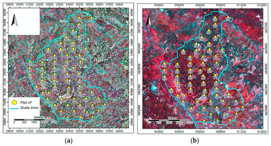
Figure 3.
Study area’s—locality of Sarnadas de S. Simão (Portugal)—infrared false color composition imagery with the inventory plots (n = 60). (a) orthophotos imagery (July 2007)—spatial resolution 0.5 m; and (b) Sentinel-2 MSI imagery (28 July 2020)—spatial resolution 10 m.
For the years from 2020 to 2022, the year of the last wildfire and after, the Sentinel-2 imagery was used. Sentinel-2 is one of the various missions of the European Union’s earth observation program called Copernicus. The first satellite, Sentinel-2A, was launched on 23 June 2015 (https://sentinels.copernicus.eu/web/sentinel/missions/sentinel-2 (accessed on 1 September 2022)). Currently, two twin Sentinel-2 satellites (A and B) offer coverage with a high spatial resolution (up to 10 m) and temporal resolution (5 days) [36].
For this study, the Sentinel-2 Multispectral Instrument (MSI) imagery, level 2A (atmospherically, radiometrically and geometrically corrected), with less than 5% of clouds coverage (Figure 3b), was downloaded for 10 dates of the years 2020–2022 (Table 3).
Table 3.
Sentinel-2A MSI imagery—date of acquisition.
The Sentinel-2 MSI imagery has 13 spectral bands covering the spectral range from 440 to 2180 nm, with spatial resolutions of 10, 20 and 60 m (Table 4).
Table 4.
Sentinel-2 MSI—spectral bands and spatial resolution [4].
The NDVI (Table 5) was computed from both sets of imagery, respectively, with a spatial resolution of 0.5 m for the orthophotos imagery and with a spatial resolution of 10 m for the Sentinel-2 imagery. The NBR (Table 5) was computed from the Sentinel-2 imagery, using the SWIR2 band with a spatial resolution of 20 m, for the dates before and after the wildfire on 13 September 2020.
Table 5.
Spectral indices—Normalized Difference Vegetation Index (NDVI) and Normalized Burn Ratio (NBR) [2].
A Geographic Information System (GIS) software, the free open-source software SAGA (System for Automated Geoscientific Analyses) (https://saga-gis.sourceforge.io/en/index.html (accessed on 1 September 2022)), was used to perform the imagery computations. The Coordinate System [EPSG 32629]: WGS84/UTM zone 29N was used.
2.2.3. Climatological Data—Local Station (2020–2022)
The closest local climatological station to the study area is located in Castelo Branco (around 40 km). The monthly climatological reports were downloaded from the official national portal of Instituto Português do Mar e da Atmosfera (IPMA) [37].
In this study, the climatological data regarding the hydrological years 2019/2020, 2020/2021 and 2021/2022 (until May) were used to obtain the evolution of monthly average temperatures (minimum and maximum °C) and total monthly precipitation (mm) (Figure 4). The accumulated monthly precipitation (mm) for each hydrological year was 708.9 mm, 695.8 mm and 326.2 mm (until May). These data were used to explain the NDVI values observed in the study area throughout 2020–2022.
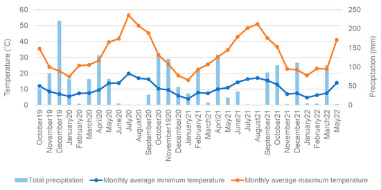
Figure 4.
Climatological data: Castelo Branco station (2020–2022)—monthly average temperatures (minimum and maximum °C) and total monthly precipitation (mm) [37].
2.3. Methods
2.3.1. Forest Inventory Plots’ NDVI Assessment
The NDVI imagery computed from the orthophotos obtained in July 2007 (Figure 5a) allowed to evaluate the average NDVI for each forest inventory plot (500 m2) using a sub-sample consisting of a kernel of 20 × 20 pixels around the plot center (100 m2) (Figure 6b).
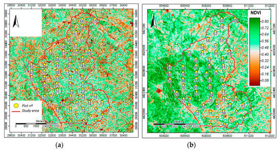
Figure 5.
Study area’s—locality of Sarnadas de S. Simão (Portugal)—NDVI imagery with the inventory plots (n = 60): (a) NDVI (July 2007)—spatial resolution 0.5 m; and (b) NDVI (28 July 2020)—spatial resolution 10 m.
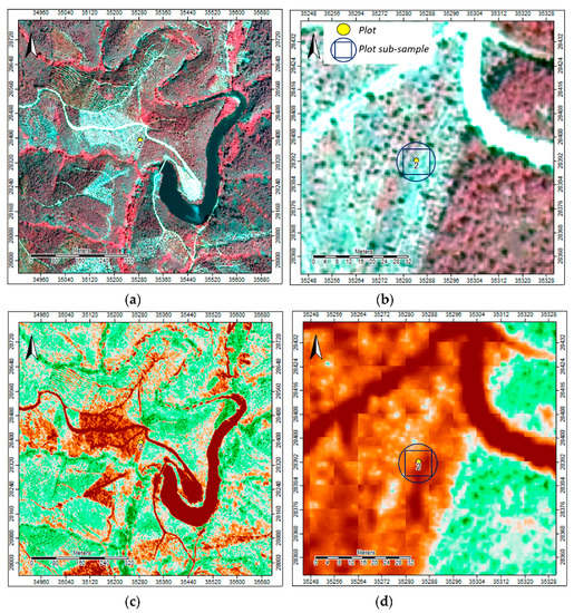
Figure 6.
Orthophoto and NDVI imagery (July 2007)—spatial resolution 0.5 m: (a) FCC showing plot n° 2; (b) FCC zoom—circular plot (500 m2) and sub-sample of a kernel of 20 × 20 pixels around the plot center (100 m2); (c) NDVI showing plot n° 2; and (d) NDVI zoom—circular plot (500 m2) and sub-sample of a kernel of 20 × 20 pixels around the plot center (100 m2) to assess plots’ average spectral vegetation index.
The NDVI imagery computed from the Sentinel-2 imagery for the 10 dates (Figure 5b—e.g., 28 July 2020) allowed to evaluate the NDVI for each forest inventory plot (500 m2) using as a sample the plot center pixel (100 m2) (Figure 7b—e.g., 28 July 2020).
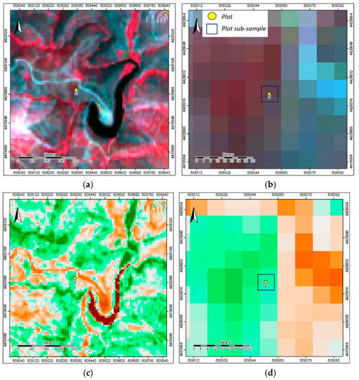
Figure 7.
Sentinel-2 and NDVI imagery (28 July 2020)—spatial resolution 10 m: (a) FCC showing plot n° 2; (b) FCC zoom—plot center pixel (100 m2); (c) NDVI showing plot n° 2; and (d) NDVI zoom—plot center pixel (100 m2) to assess plot spectral vegetation index.
2.3.2. NDVI and Maritime Pine Production (2007)
The WEKA (Waikato Environment for Knowledge Analysis) open-source software was used for modeling purposes [38,39]. Maritime pine plots’ average NDVI in 2007, computed in a sub-sample of a kernel of 20 × 20 pixels around the plot center (100 m2), were first explored regarding this species’ dendrometric characteristics (Table 2). In the WEKA software, the search method “Rankers” under the “Correlation Attribute Evaluation” was used as it provides a selection ranking technique for the predictors’ inclusion in the final regression model by measuring the correlation (Pearson) between the predictor and the class.
Afterward, Maritime pine wood production (V) and aboveground biomass production (Wa) were fitted by simple linear regression using the plots’ average NDVI as the explanatory variable. Due to the poor correlation observed between the plots’ average NDVI and V and Wa, the transformed NDVI, set as NDVI_a = NDVI (t/R) with R = 40 year, was also essayed [12]. In the WEKA software, under “Classify,” several modeling algorithms are available, namely simple linear regression. WEKA software provides k-fold cross-validation to test the algorithm’s accuracy by dividing the data set into k subsets. One of these subsets is randomly selected as the test set, and the other k-1 subset constitutes the training sample in each run. The models’ fitting performance is assessed using statistics such as the pseudo-coefficient of determination (R2), the mean absolute error (MAE) and the root mean squared error (RMSE).
2.3.3. NDVI by Cover Type (2007 and 2020–2021)
The plots’ average NDVI in 2007 was also used to explore the differences between cover types (e.g., shrub; Maritime pine regeneration; Maritime pine; and pure and mixed Eucalyptus).
Afterward, the cover type in each plot in 2020 was updated using the Portuguese official land cover map COS 2018 [30] (Figure 1d) and by Google Earth imagery photo interpretation (May–Jun 2019). Again, the plots’ NDVI was used to explore the differences between cover types (e.g., shrub; Maritime pine; Eucalyptus) throughout the 2020 growing season (10 March 2020, 29 May 2020, 28 June 2020, 28 July 2020 and 26 September 2020).
A two-sample Z-test for means, at a confidence level of 95%, was performed to compare the plots’ average NDVI by cover type in July 2007 and on 28 July 2020. Then, the NDVI ann-min and CV method was used to differentiate the cover types throughout the 2020 growing season by its NDVI time curve [23]. Then, a further detailed analysis was also performed for plots of specific cover types throughout the 2020 growing season by its NDVI time curve.
2.3.4. Burn Severity and Post-Fire Vegetation Recovery Monitoring (2020–2022)
In the year 2020, a wildfire on 13 September affected the study area (Figure 2d). Fire burn scars were explored using the NBR pre-fire (6 September 2020) and post-fire (26 September 2020). Then, the difference in the NBR between the two dates was obtained. After, the dNBR was used to classify burn severity according to the levels proposed by the European Forest Fire Information Service (EFFIS) (Table 6) [4]. The Portuguese official burned area map of 2020 (Figure 2d) was overlaid on the dNBR image and used as a reference.
Table 6.
Burn severity—differenced Normalized Burn Ratio (dNBR) thresholds proposed by the European Forest Fire Information Service (EFFIS) [4].
The NDVI was used to monitor vegetation recovery post-fire (26 September 2020) during three six-month periods from 2021 to 2022 (15 March 2021, 21 September 2021 and 9 May 2022). As it is known, the NDVI values range from −1 to 1, where water surfaces, manmade structures, rocks, clouds, and snow correspond to negative values; bare soil usually falls within the 0.1–0.2 range and plants will always have positive values between 0.2 and 1. Particularly, a healthy, dense vegetation canopy should be above 0.5, and sparse vegetation will most likely fall within the 0.2 to 0.5 range [40]. Thus, the NDVI imagery was reclassified considering three greenness classes (Table 7) to monitor vegetation recovery post-fire.
Table 7.
Normalized Difference Vegetation Index (NDVI) thresholds for greenness classes [40].
In addition, the burned plots in the 2020 wildfire were monitored to understand the NDVI pattern regarding its burn severity levels between 2020 and 2022 (10 March 2020, 29 May 2020, 28 June 2020, 28 July 2020, 6 September 2020, 26 September 2020, 15 March 2021, 14 May 20021, 21 September 2021, 30 March 2022 and 9 May 2022).
3. Results
3.1. NDVI and Maritime Pine Production (2007)
The correlation between the Maritime pine plots’ average NDVI and stand variables was poor (less than 0.22). The best five variables correlation were the following: G (−0.22); Sh25 (−0.18); N (0.17); Wl (0.17); and Wr (0.17). The variables G and N are absolute measures of stand density, the variable Sh25 is an indicator of site productivity, and the variables Wl and Wr give an insight, respectively, of tree crown photosynthesis capability and tree roots growing space in the stand. All these variables are important parameters that determine stand production.
Regarding the plots’ average NDVI correlation with wood production (V) and aboveground biomass production (Wa), it was found to be very low (around 0.03). Only, using the transformed NDVI_a, correlations between 0.72 and 0.73 were achieved. Therefore, as expected, the modeling efficiency of the linear models V = f(NDVI_a) and Wa = f(NDVI_a) was not very high (R2 around 60%) (Figure 8a,b).
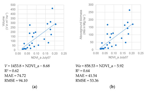
Figure 8.
Mature Maritime pine naturally regenerated production (V and Wa) and NDVI_a models: (a) V = f(NDVI_a)—plot, model, and fitting and prediction statistics; and (b) Wa = f(NDVI_a)—plot, model, and fitting and prediction statistics.
These Maritime pine stands were established by natural regeneration, and, in 2007, they were mainly under-stocked or very under-stocked. The inexistent or inappropriate silvicultural intervention may explain this under-stocked condition, such as the application of a single and late high-grade thinning without having stand stability under consideration [32]. Both the establishment regime of these stands (natural regeneration, thus with irregular spacing) and the absence of an appropriate stand management prescription convey a high variability of the development conditions between stands and as well in horizontal and vertical stands’ structures (diametric and height distributions) (Table 2). This variability has a negative impact on the modeling efforts, as was verified. These stands also have a substantial understory coverage (average around 54%) that may have influenced the observed NDVI values.
3.2. NDVI by Cover Type (2007 and 2020–2021)
In 2007, the plots’ average NDVI by cover type (e.g., S—Shrub; MP—Maritime pine; MPr—Maritime pine regeneration; and E—pure and mixed Eucalypts) showed high variation, thus not allowing good discrimination between covers (Figure 9; Appendix A—Figure A1).
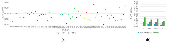
Figure 9.
Forest inventory plots’ NDVI (2007): (a) plots’ NDVI by cover types (S—Shrub; MP—Maritime pine; MPr—Maritime pine regeneration; and E—pure and mixed Eucalypts; and (b) NDVI variability by cover type.
In 2020, the plots’ NDVI by cover type (e.g., shrub, Maritime pine and Eucalyptus) showed high variation again, thus not allowing good discrimination between them (Figure 10).
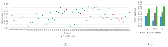
Figure 10.
Forest inventory plots’ NDVI (28 July 2020): (a) plots’ NDVI by cover types (S—Shrub; MP—Maritime pine; and E—Eucalypts); and (b) NDVI variability by cover type.
The results of the two sample Z-test for means to compare the plots’ average NDVI by cover type, either in July 2007 and on 28 July 2020, indicated that no statistically significant differences were found, at a 95% confidence level, between mature Maritime pine and the other cover types.
The analysis of plots’ NDVI by cover type throughout the growing season (March to September 2020) showed a peak (greening) in early spring and early fall and a hole (browning—NDVI ann-min) in July for the three cover types (Figure 11a).
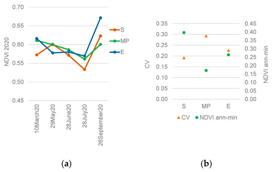
Figure 11.
Forest inventory plots’ NDVI during the 2020 growing season (March–September 2020): (a) Plots’ mean NDVI by cover type (S—Shrub; MP—Maritime pine; and E—Eucalypts); and (b) Annual minimum NDVI and coefficient of variation (CV) by cover type.
When analyzing the annual minimum NDVI (NDVI ann-min) with the coefficient of variation (CV) throughout the 2020 growing season for each cover type (e.g., shrub, Maritime pine and Eucalyptus), significant differences were shown (Figure 11b). Shrubs showed high NDVI ann-min and intermediate CV. Eucalypts plantations showed both intermediate NDVI ann-min and CV, and Maritime pine naturally regenerated forest showed low NDVI ann-min and high CV (Figure 11b).
The detailed analysis of plots’ NDVI allowed to stratify plots of specific cover types by stand development and fire occurrence (Figure 12a) as follows: Eucalypts mature (plot n° 44), young (plot n° 48), and post-fire (plot n° 49); Maritime pine mature (plot n° 24), young (plot n° 37), and post-fire (plot n° 6); and shrubs post-fire (plot n° 17—Arbutus unedo, plot n° 51—Erica sp. And plot n° 54—Cytisus sp.). All plots were burned in the 2003 wildfire except for plot n° 24 (Maritime pine mature). Most of the plots were also burned in the 2017 wildfire except for plots n° 24 (Maritime pine mature), plot n° 37 (Maritime pine young regeneration), plot n° 44 (Eucalypts mature) and plot n° 48 (Eucalypts young) (Appendix A—Table A1, Figure A2, Figure A3 and Figure A4).
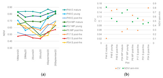
Figure 12.
Chosen forest inventory plots’ NDVI throughout the 2020 growing season (March–September 2020): (a) Plots’ mean NDVI by cover type (Eucalypts mature, young, and post-fire; Maritime pine mature, young, and post-fire; and Shrubs and shrubs post-fire); and (b) Annual minimum NDVI and coefficient of variation (CV) by cover type.
These nine plots’ NDVI were analyzed regarding their NDVI time curve throughout the 2020 growing season (March–September 2020) (Figure 12a), and their NDVI ann-min and CV were evaluated (Figure 12b).
The nine plots’ cover types could be ranked by decreasing NDVI values as follows: mature Eucalypts plantations (plot n° 44: NDVI = 0.82; CV = 0.02), young Maritime pine regeneration (plot n° 37: NDVI = 0.75; CV = 0.07), mature Maritime pine (plot n° 24: NDVI = 0.68; CV = 0.05), young Eucalypts plantations (plot n° 48: NDVI = 0.56; CV = 0.15), Strawberry tree shrubland (plot n° 17: NDVI = 0.56; CV = 0.17), Eucalypts plantations post-fire (plot n° 49: NDVI = 0.49; CV = 0.15), Maritime pine post-fire (plot n° 6: NDVI = 0.48; CV = 0.13), tall shrubland (plot n° 54: NDVI = 0.46; CV = 0.16) and short shrubland (plot n° 51: NDVI = 0.44; CV = 0.11) (Figure 12b).
3.3. Burn Severity and Post-Fire Vegetation Recovery Monitoring (2020–2022)
The fire burn scar of the wildfire on 13 September 2020 was extracted using the dNBR (Figure 13c) between the pre-fire date (Figure 13a—6 September 2020) and the post-fire date (Figure 13b—26 September 2020). This allowed the observation of a very high burn severity throughout all the study areas burned areas (Figure 13).
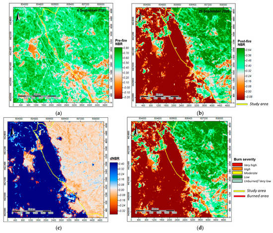
Figure 13.
Wildfire—13 September 2020: (a) NBR 6 September 2020; (b) NBR 26 September 2020 (fire scar in shades of brown); and (c) dNDVI 6–26 September 2020 (shades of blue) and official 2020 fire limits (in red); and (d) dNBR levels for burn severity by EFFIS and official 2020 fire limits (in red).
Forest vegetation recovery post-fire (after 13 September 2020) showed that in early spring (15 March 2021), the recovery was not very significant (Figure 14a,d). However, substantial recovery was already observed in late summer (21 September 2021) (Figure 14b,e). In the following year, early spring (9 May 2022), an overall decrease in greenness was observed (Figure 14c,f) because of a very dry winter (Figure 4—January and February 2022).
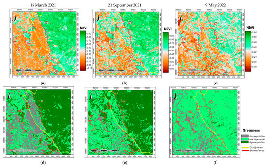
Figure 14.
Post-fire recovery—13 September 2020 (fire limits in red): (a) NDVI 15 March 2021; (b) NDVI 21 September 2021; (c) NDVI 9 May 2022; (d) NDVI classes 15 March 2021; (e) NDVI classes 21 September 2021; and (f) NDVI classes 9 May 2022.
Only four plots (plots n° 26, 35, 40 and 45) were burned in the 2020 wildfire but with different fire severities (Figure 15 and Figure 16).
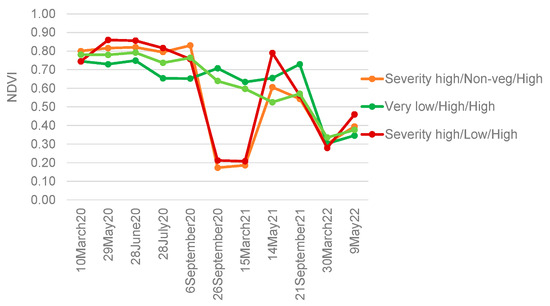
Figure 15.
Forest inventory burned plots in 2020: NDVI (March 2020–May 2021).
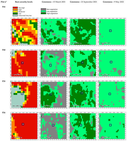
Figure 16.
Forest inventory burned plots (marked in blue) in 2020—post-fire recovery: burn severity levels; NDVI classes 15 March 2021; NDVI classes 21 September 2021; and NDVI classes 9 May 2022.
These plots were also burned in the 2003 and 2017 wildfires (Appendix A—Table A1, Figure A2 and Figure A4). In 2007, the plot n° 26 land cover was shrub (50% Erica sp.), plot n° 35 was shrub (50% Cytisus sp.), plot n° 40 was shrub (60% Arbutus unedo) and plot n° 45 was shrub (50% Cistus sp.) (Appendix A—Figure A5). Again, in early spring (15 March 2021), these plots’ landcover recovery was not very significant, followed in late summer (21 September 2021) by a substantial recovery, and in the following year, early spring (9 May 2022) by an overall decrease in greenness (Figure 15 and Figure 16) due to a very dry winter (Figure 4—January and February 2022).
4. Discussion
This study’s research hypothesis was that the use of remotely sensed spectral indices would be effective: (1) to model Maritime pine production (wood and biomass) using the NDVI as the explanatory variable; (2) to differentiate evergreen coniferous forests (e.g., Maritime pine), evergreen broadleaved forests (e.g., Eucalypts), and shrubland by their NDVI time curve patterns; and (3) to monitor vegetation disturbances such as fire events and/or stress by weather conditions variations using the NDVI and the NBR.
Regarding the first purpose of modeling mature Maritime pine wood production (V) and aboveground biomass production (Wa), the NDVI was successfully achieved with a fitting efficiency of around 60% using the transformed NDVI by stand age (NDVI_a) as the explanatory variable. Indeed, the NDVI has been used for the quantitative assessment of vegetation and biomass in several other studies [11]. Moreover, the results obtained in this study are consistent with other studies that used the NDVI with forest inventory data to model wood production and biomass [12,13]. Wherein the wood production (m3 ha−1) of planted forests of Eucalypts and Pine was modeled using a linear model of NDVI_a as the explanatory variable with fitting efficiencies of 79% and 60%, respectively, for each species [12]. However, other studies pointed out that better efficiencies in modeling forest aboveground biomass were achieved when a fusion of remote sensing data sources (e.g., hyperspectral, LiDAR and RADAR imagery) was used [41,42]. Moreover, the NDVI was used to monitor forest plantations’ wood quality due to its positive correlation with a uniformity index that is stand height-based [14].
Moving to the second purpose, which focused on the use of the NDVI to differentiate cover types, it should be first noted that the NDVI computed from the orthophoto imagery (spatial resolution of 0.5 m) was found to be much lower than the NDVI computed from the Sentinel-2 imagery (spatial resolution of 10 m). This difference is consistent with the findings of a study that compared the NDVI values of three land cover types (e.g., forest, golf course grass and airport runway in concrete) computed from one aerial and four free satellite data sources acquired in autumn between 2016 and 2019. In that study, the NDVI computed from the USDA National Agriculture Imagery Program aerial photography (spatial resolution of 0.6 m) for vegetation covers was found to be much lower when compared to the one computed from the Sentinel-2 surface reflectance data (spatial resolution of 10 m) [19].
In fact, continuous efforts have been made to compare NDVI values acquired with different sensors. But as is known, sensor types are characterized by varying sensor technologies and platforms, which differentiate remote sensing data sets. Thus, due to differences in bandwidths, spatial resolutions and data processing, different sensors can deliver notably different NDVI behaviors, particularly between spaceborne and airborne sensors [19]. Nevertheless, the NDVI effectively expresses vegetation status and quantifies vegetation attributes. Still, aspects such as the atmospheric effect, saturation phenomenon, and sensor factors must be considered to avoid its misuse, especially in unmanned aerial systems (Drones) applications [19].
Secondly, regarding plots’ average NDVI by cover type, computed from the orthophoto imagery of July 2007, a high variation was observed, thus not allowing discrimination between covers. The same was verified in the plots’ average NDVI by cover type computed from the Sentinel-2 imagery of 28 July 2020. Moreover, no significant statically differences were found between mature Maritime pine and the other types of cover under analysis in July 2007 and on 28 July 2020. Therefore, indicating that features other than the cover type, such as stand development stage (young vs. mature) and fire occurrence (unburned vs. burned), must be considered to differentiate them. In effect, it is known that NDVI measures vegetation greenness and is related to structural properties of plants (e.g., leaf area index and green biomass) but also to properties of vegetation productivity (e.g., absorbed photosynthetic active radiation and foliar nitrogen) [21].
Even so, the NDVI ann-min and CV approach proved to be efficient in differentiating cover types using its NDVI time curve throughout the growing season. As a result, shrubs showed a high NDVI ann-min and intermediate CV (NDVI = 0.40; CV = 0.19), Eucalypts plantations showed both intermediate NDVI ann-min and CV (NDVI = 0.26; CV = 0.23) and Maritime pine naturally regenerated forest showed a low NDVI ann-min and high CV (NDVI = 0.17; CV = 0.29). These results are consistent with the theoretical knowledge that coniferous forests (e.g., Maritime pine) have a lower NIR reflectance when compared to broadleaved forests (e.g., Eucalypts) [10,43] and hence respectively, have lower and higher NDVI values. Regarding Maritime pine, the higher CV may be explained due to these stands being established by natural regeneration (irregular tree spacing), resulting in high variability in density and biomass. Conversely, Eucalypts are established by plantations following a well-defined silvicultural prescription (e.g., regular spacing of 3 × 2 or 3 × 3 m, that is, an initial stand density of 1111 to 1667 trees per ha).
When considering the cover types stratification by stand development stage and by the occurrence of fire, a ranking by decreasing NDVI values was obtained as follows: mature Eucalypts plantations (NDVI = 0.82; CV = 0.02), young Maritime pine regeneration (NDVI = 0.75; CV = 0.07), mature Maritime pine (NDVI = 0.68; CV = 0.05), young Eucalypts plantations (NDVI = 0.56; CV = 0.15), Strawberry tree shrubland (NDVI = 0.56; CV = 0.17), Eucalypts plantations pos-fire (NDVI = 0.49; CV = 0.15), Maritime pine post-fire (NDVI = 0.48; CV = 0.13), tall shrubland (NDVI = 0.46; CV = 0.16) and short shrubland (NDVI = 0.44; CV = 0.11).
As expected, mature Eucalypts plantations showed higher NDVI than mature Maritime pine naturally regenerated. Eucalypts plantations post-fire and Maritime pine post-fire also showed the same trend. But the same was not true for young Eucalypts plantations, and young Maritime pine naturally regenerated due to the type of stand establishment (plantation vs. natural regeneration). In young Eucalypts plantations, the mixed pixel problem may explain the low NDVI value as, at the plantation stage, substantial bare soil is exposed (spatial resolution 10 × 10 m) [23]. Conversely, the establishment of young maritime pine by intense natural regeneration and providing complete ground coverage had a high NDVI value.
In view of the third purpose focused on the use of NDVI and NBR to monitor vegetation disturbances (e.g., fire events and/or low precipitation). The dNBR allowed to map the 2020 burned area and assess the burn severity levels. It was possible to observe that the mountain area in the study area’s western zone had burned with high burn severity. Indeed, the NBR computed from the Sentinel-2 MSI short-wave infrared 2—SWIR2 produced good results for detecting burned areas and obtaining the burning severity levels [3,4,17,18]. Several studies have proved that Sentinel-2 MSI imagery can be used to differentiate burned areas and burning severity [17]. Wherein the most suitable MSI bands to detect burned areas were the 20 m NIR, SWIR and red-edge bands [18]. Indeed, the NBR computed with the SWIR2 band produced the best results for detecting burned areas and separating burning severity levels in the Sierra de Gata region (Spain) [17]. In Galicia (Spain), to carry out a restoration campaign after the 2017 forest fires, the dNDVI and dNBR of pre-fire and post-fire dates were used. Moreover, the burn severity levels obtained by reclassifying the dNBR were validated with field data showing good accuracy [3]. The NBR was also used to assess the burn severity levels according to the EFFIS of the fires that occurred in October 2017 in Spain and Portugal. This study revealed that the use of the Sentinel-2 imagery improved the burned area estimation and that the burn severity levels obtained showed a high correlation with those produced by EFFIS [4]. Both the NDVI and the NBR were used successfully to assess the 2016 post-fire conditions in Madeira (Portugal) [36].
Regarding the use of the NDVI to monitor vegetation post-fire recovery, it was observed that recovery was lower in higher burn severity levels (e.g., dNBR class very high). During the period under analysis in this study, this mountain area was irregularly burned in 2003, 2017 and 2020. As a result, it is currently dominated by shrubland (mainly Arbutus unedo), which has a good recovery capability. Eucalypts plantations also have a good recovery capability post-fire. In opposition, the existent Maritime pine natural regeneration was burned, so it is very unlikely that this species will occur in this area again in the short term. Since Maritime pine is a light pioneer species, viable seed production occurs later in stands of 15 to 20 years old, ensuring the desirable natural regeneration [44].
This has been observed in other Maritime pine regenerated areas that have been affected by a short cycle of wildfires. Indeed, fire occurrence affects landscape patterns and dynamics by changing vegetation type and structure and the soil processes according to the fire adaptations of each ecosystem. Moreover, landowners’ decisions as a response to the presence (or absence) of fire are likely to also have a determinant role in post-fire land cover dynamics as wildfires offer either an opportunity for land cover change or might be a discouraging element, leading land owners to stop managing their land [45]. For instance, in Portugal, most of the Maritime pine burned area has been converted into shrubland, pastures, and Eucalypts plantations [29].
When analyzing the burned plots’ NDVI in the 2020 wildfire, a strong reduction in NDVI was observed when the burn severity was high, conversely to a small reduction when the burn severity was low and moderate. Nevertheless, all plots observed a good recovery in the next spring. Due to a very dry winter, an important reduction in NDVI was again observed in the following spring in all plots. Indeed, the 2021/2022 hydrological year (until May) was the fourth driest year since 1931 [46]. These results are consistent with other studies that indicate it as the cause for the NDVI decrease in the impact of fire and/or low precipitation (NDVI anomalies) [3,15,21,24,25].
Finally, despite the good results that the NBR and NDVI have shown in measuring fire-induced vegetation loss, these indices and others should be tested against field data (e.g., canopy scorch, tree mortality, ground char, fuels consumption, ash cover) across a variety of vegetation biomes and fire regimes to determine where they are most useful and what they actually measure in terms of post-fire ecological effects [26].
5. Conclusions
The main conclusions of this study were as follows: (1) the linear models of Maritime pine production (wood and biomass) with NDVI_a showed a fitting efficiency of around 60%; (2) the NDVI values computed from the orthophoto imagery were found not to be comparable to those computed from the Sentinel-2 imagery due to differences in sensors, bandwidths and spatial resolutions; (3) the plots’ NDVI values by cover type, both in 2007 and 2020, showed high variability and no statistically significant differences were found between mature Maritime pine, Eucalypts and shrubland. But the differentiation between cover types by stand development stage and by fire occurrence was possible when the NDVI-CV method was applied to the NDVI time curve throughout the 2020 growing season. Consequently, cover types were ranked by decreasing NDVI values as follows: mature Eucalypts plantations, young Maritime pine regeneration, mature Maritime pine, young Eucalypts plantations, Strawberry tree shrubland, Eucalypts plantations pos-fire, Maritime pine post-fire, tall shrubland, and short shrubland; and (4) the 2020 burned area was well detected by the dNBR, allowing to assess the burn severity levels. The NDVI and the NBR showed that vegetation post-fire recovery was lower in higher burn severity levels. Due to the sequence of short cycles of wildfires in the study area, Maritime pine areas have lost their natural regeneration capability. Shrubland (e.g., Arbutus unedo) had a very significant post-fire recovery a year later, and the burned plots’ NDVI time curve during 2000–2022 clearly showed the reduction of NDVI due to the impact of the wildfire (13 September 2020) and last winter’s low precipitation (January and February 2022).
In sum, NDVI and NBR proved to be effective in differentiating cover types and as monitoring tools to assist in the evaluation of forests and shrubland conditions. Therefore, it is crucial to keep investigating the species’ unique spectral characteristics based on its phenology to extract them from other species. In that view, further research is still needed using more robust time-series data to define species growing pattern NDVI time curves and its subsequent validation by field data and other ancillary data (e.g., precipitation) to support vegetation mapping and monitoring.
Funding
This study was funded by CERNAS-IPCB [UIDB/00681/2020] funding from the Foundation for Science and Technology (Fundação para a Ciência e Tecnologia—FCT)].
Institutional Review Board Statement
Not applicable.
Informed Consent Statement
Not applicable.
Conflicts of Interest
The author declares no conflict of interest.
Appendix A
Table A1.
Forest inventory plots (2007): fires in grey (1975–1989, 1990–1999, 2000–2009, 2017 and 2020), land cover (COS 1995, 2007 and 2018) and plot cover (2007).
Table A1.
Forest inventory plots (2007): fires in grey (1975–1989, 1990–1999, 2000–2009, 2017 and 2020), land cover (COS 1995, 2007 and 2018) and plot cover (2007).
| Plot n° | Fires 1975–1989 | Fires 1990–1999 | COS 1995 | Fires 2000–2009 | COS 2007 | Plot cover | Fire 2017 | COS 2018 | Fire 2020 |
|---|---|---|---|---|---|---|---|---|---|
| 1 | E | E | MP | E | |||||
| 2 | MP | E | E | E | |||||
| 3 | MP | MP | MP | MP | |||||
| 4 | MP | MP | MP | E | |||||
| 5 | MP | MP | MP | MP | |||||
| 6 | MP | S | MP | MP | |||||
| 7 | MP | MP | MP | MP | |||||
| 8 | MP | MP | ExMP | MP | |||||
| 9 | MP | MP | MP | MP | |||||
| 10 | MP | MP | MP | MP | |||||
| 11 | MP | MP | MP | MP | |||||
| 12 | MP | MP | MP | MP | |||||
| 13 | MP | MP | MP | MP | |||||
| 14 | MP | MP | MP | MP | |||||
| 15 | MP | MP | MP | MP | |||||
| 16 | A | A | MP | A | |||||
| 17 | MP | S | S | MP | |||||
| 18 | MP | MP | MP | MP | |||||
| 19 | MP | MP | MP | MP | |||||
| 20 | MP | MP | MP | MP | |||||
| 21 | MP | MP | MP | MP | |||||
| 22 | MP | MP | MP | MP | |||||
| 23 | MP | MP | MP | MP | |||||
| 24 | MP | MP | MP | MP | |||||
| 25 | MP | MP | MPxE | MP | |||||
| 26 | MP | MP | S | MP | |||||
| 27 | MP | MP | MPxE | MP | |||||
| 28 | MP | MP | MP | MP | |||||
| 29 | S | S | MPr | S | |||||
| 30 | A | A | S | A | |||||
| 31 | MP | MP | MP | MP | |||||
| 32 | MP | MP | MP | MP | |||||
| 33 | MP | MP | MP | MP | |||||
| 34 | MP | MP | MPr | MP | |||||
| 35 | MP | S | S | MP | |||||
| 36 | MP | MP | MPr | S | |||||
| 37 | MP | MP | MPr | MP | |||||
| 38 | S | S | S | E | |||||
| 39 | MP | S | MPr | MP | |||||
| 40 | MP | S | S | MP | |||||
| 41 | MP | S | MPr | E | |||||
| 42 | MP | MP | MPr | MP | |||||
| 43 | MP | MP | MPr | MP | |||||
| 44 | MP | E | S | E | |||||
| 45 | MP | S | S | MP | |||||
| 46 | MP | S | S | E | |||||
| 47 | MP | E | MPr | E | |||||
| 48 | MP | MP | MPr | E | |||||
| 49 | MP | MP | S | E | |||||
| 50 | MP | MP | MPr | MP | |||||
| 51 | MP | S | MPr | S | |||||
| 52 | MP | S | MPr | S | |||||
| 53 | MP | MP | MPr | MP | |||||
| 54 | MP | S | S | S | |||||
| 55 | MP | MP | MPr | S | |||||
| 56 | MP | MP | MPr | S | |||||
| 57 | MP | E | MPr | E | |||||
| 58 | MP | S | MPr | MP | |||||
| 59 | MP | S | S | S | |||||
| 60 | MP | S | S | MP |
Legend: E—Eucalypts; ExMP—Mixed Eucalypts and Maritime pine; MPxE—Mixed Maritime pine and Eucalypts; MP—Maritime pine; MPr—Maritime pine regeneration; S—Shrubs; and A—Agriculture; fire occurrence marked in grey.
Table A2.
Individual tree biomass prediction equations for Maritime pine in Portugal [35].
Table A2.
Individual tree biomass prediction equations for Maritime pine in Portugal [35].
| Variable | Equation |
|---|---|
| Stem under bark | |
| Bark | |
| Branches | |
| Leaves | |
| Roots | |
| Aboveground | |
| Tree |
Legend: d—individual tree diameter, over bark, at breast height (1.30 m above ground) (cm); h—tree total height (m); ws—stem biomass under bark (Kg); wb—bark biomass (Kg); wbr—branch biomass (Kg); wl—leaves biomass (Kg); wa—aboveground biomass (Kg); wr—roots biomass (Kg); and w—tree biomass (Kg).

Figure A1.
Orthophotos imagery (July 2007): plots (circled in orange) with NDVI maximum and minimum by cover type.
Figure A1.
Orthophotos imagery (July 2007): plots (circled in orange) with NDVI maximum and minimum by cover type.


Figure A2.
Google Earth imagery (May–June 2019): (a) chosen plots by cover type (marked in orange); and (b) plots that burned in 2020 (circled in orange).
Figure A2.
Google Earth imagery (May–June 2019): (a) chosen plots by cover type (marked in orange); and (b) plots that burned in 2020 (circled in orange).


Figure A3.
Orthophotos imagery (July 2007): chosen plots (circled in orange).
Figure A3.
Orthophotos imagery (July 2007): chosen plots (circled in orange).


Figure A4.
Sentinel-2 imagery (28 July 2020): chosen plots (circled in orange).
Figure A4.
Sentinel-2 imagery (28 July 2020): chosen plots (circled in orange).


Figure A5.
Temporal perspective of the plots (circles in orange) that burned in 2020: (a) orthophotos imagery July 2007; (b) Sentinel-2 imagery (28 July 2020); and (c) Sentinel-2 imagery (9 May 2022).
Figure A5.
Temporal perspective of the plots (circles in orange) that burned in 2020: (a) orthophotos imagery July 2007; (b) Sentinel-2 imagery (28 July 2020); and (c) Sentinel-2 imagery (9 May 2022).

References
- Arroyo, L.A.; Pascual, C.; Manzanera, J.A. Fire models and methods to map fuel types: The role of remote sensing. For. Ecol. Manag. 2008, 256, 1239–1252. [Google Scholar] [CrossRef]
- Fernández-Manso, A.; Fernández-Manso, O.; Quintano, C. SENTINEL-2A red-edge spectral indices suitability for discriminating burn severity. Int. J. Appl. Earth Obs. Geoinf. 2016, 50, 170–175. [Google Scholar] [CrossRef]
- Sobrino, J.A.; Llorens, R.; Fernández, C.; Fernández-Alonso, J.M.; Vega, J.A. Relationship between forest fires severity measured in situ and through remotely sensed spectral indices. Forests 2019, 10, 457. [Google Scholar] [CrossRef]
- Llorens, R.; Sobrino, J.A.; Fernández, C.; Fernández-Alonso, J.M.; Vega, J.A. A methodology to estimate forest fires burned areas and burn severity degrees using Sentinel-2 data. Application to the October 2017 fires in the Iberian Peninsula. Int. J. Appl. Earth Obs. Geoinf. 2021, 95, 102243. [Google Scholar] [CrossRef]
- García, M.; Riaño, D.; Chuvieco, E.; Salas, J.; Danson, F.M. Multispectral and LiDAR data fusion for fuel type mapping using Support Vector Machine and decision rules. Remote Sens. Environ. 2011, 115, 1369–1379. [Google Scholar] [CrossRef]
- Moreira, F.; Viedma, O.; Arianoutsou, M.; Curt, T.; Koutsias, N.; Rigolot, E.; Barbati, A.; Corona, P.; Vaz, P.; Xanthopoulos, G.; et al. Landscape—wildfire interactions in southern Europe: Implications for landscape management. J. Environ. Manag. 2011, 92, 2389–2402. [Google Scholar] [CrossRef]
- Lasaponara, R.; Lanorte, A. Remotely sensed characterization of forest fuel types by using satellite ASTER data. Int. J. Appl. Earth Obs. Geoinf. 2007, 9, 225–234. [Google Scholar] [CrossRef]
- Xie, Y.; Sha, Z.; Yu, M. Remote sensing imagery in vegetation mapping: A review. J. Plant Ecol. 2008, 1, 9–23. [Google Scholar] [CrossRef]
- Fornacca, D.; Ren, G.; Xiao, W. Evaluating the best spectral indices for the detection of burn scars at several post-fire dates in a Mountainous Region of Northwest Yunnan, China. Remote Sens. 2018, 10, 1196. [Google Scholar] [CrossRef]
- Lillesand, T.; Kiefer, R. Remote Sensing and Image Interpretation; John Wiley & Sons: New York, NY, USA; Chichester, UK; Brisbane, Australia; Toronto, ON, Canada; Singapore, 1994; 376p. [Google Scholar]
- Kumar, L.; Sinha, P.; Taylor, S.; Alqurashi, A.F. Review of the use of remote sensing for biomass estimation to support renewable energy generation. J. Appl. Remote Sens. 2015, 9, 97696. [Google Scholar] [CrossRef]
- Berra, E.F.; Fontana, D.C.; Kuplich, T.M. Tree Age As Adjustment Factor to Ndvi. Rev. Árvore 2017, 41, e410307. [Google Scholar] [CrossRef]
- Gizachew, B.; Solberg, S.; Næsset, E.; Gobakken, T.; Bollandsås, O.M.; Breidenbach, J.; Zahabu, E.; Mauya, E.W. Mapping and estimating the total living biomass and carbon in low-biomass woodlands using Landsat 8 CDR data. Carbon Balance Manag. 2016, 11, 13. [Google Scholar] [CrossRef] [PubMed]
- Santos, L.H.O.; Ramirez, G.M.; Roque, M.W.; de Lima Chaves, M.P.; Diaz, L.M.G.R.; Chaves, S.P. Correlação entre uniformidade e NDVI em povoamentos de Tectona grandis L. f. BIOFIX Sci. J. 2019, 4, 130. [Google Scholar] [CrossRef]
- Erasmi, S.; Klinge, M.; Dulamsuren, C.; Schneider, F.; Hauck, M. Modelling the productivity of Siberian larch forests from Landsat NDVI time series in fragmented forest stands of the Mongolian forest-steppe. Environ. Monit. Assess. 2021, 193, 200. [Google Scholar] [CrossRef]
- Mendes, T.R.S.; Miguel, E.P.; Vasconcelos, P.G.A.; Valadão, M.B.X.; Rezende, A.V.; Matricardi, E.A.T.; Angelo, H.; Gatto, A.; Nappo, M.E. Use of aerial image in the estimation of volume and biomass of Eucalyptus sp. forest stand. Aust. J. Crop Sci. 2020, 14, 286–294. [Google Scholar] [CrossRef]
- Amos, C.; Petropoulos, G.P.; Ferentinos, K.P. Determining the use of Sentinel-2A MSI for wildfire burning & severity detection. Int. J. Remote Sens. 2019, 40, 905–930. [Google Scholar] [CrossRef]
- Huang, H.; Roy, D.P.; Boschetti, L.; Zhang, H.K.; Yan, L.; Kumar, S.S.; Gomez-Dans, J.; Li, J. Separability analysis of Sentinel-2A Multi-Spectral Instrument (MSI) data for burned area discrimination. Remote Sens. 2016, 8, 873. [Google Scholar] [CrossRef]
- Huang, S.; Tang, L.; Hupy, J.P.; Wang, Y.; Shao, G. A commentary review on the use of normalized difference vegetation index (NDVI) in the era of popular remote sensing. J. For. Res. 2021, 32, 1–6. [Google Scholar] [CrossRef]
- Veraverbeke, S.; Lhermitte, S.; Verstraeten, W.W.; Goossens, R. The temporal dimension of differenced Normalized Burn Ratio (dNBR) fire/burn severity. Remote Sens. Environ. 2010, 114, 2548–2563. [Google Scholar] [CrossRef]
- Forkel, M.; Carvalhais, N.; Verbesselt, J.; Mahecha, M.D.; Neigh, C.S.R.; Reichstein, M. Trend Change detection in NDVI time series: Effects of inter-annual variability and methodology. Remote Sens. 2013, 5, 2113–2144. [Google Scholar] [CrossRef]
- Zhao, X.; Xu, P.; Zhou, T.; Li, Q.; Wu, D. Distribution and variation of forests in china from 2001 to 2011: A study based on remotely sensed data. Forests 2013, 4, 632–649. [Google Scholar] [CrossRef]
- Yang, Y.; Wu, T.; Wang, S.; Li, J.; Muhanmmad, F. The NDVI-CV Method for mapping evergreen trees in complex urban areas using reconstructed landsat 8 time-series data. Forests 2019, 10, 139. [Google Scholar] [CrossRef]
- Navarro, A.; Catalao, J.; Calvao, J. Assessing the use of Sentinel-2 time series data for monitoring Cork Oak decline in Portugal. Remote Sens. 2019, 11, 2515. [Google Scholar] [CrossRef]
- Petropoulos, G.P.; Griffiths, H.M.; Kalivas, D.P. Quantifying spatial and temporal vegetation recovery dynamics following a wildfire event in a Mediterranean landscape using EO data and GIS. Appl. Geogr. 2014, 50, 120–131. [Google Scholar] [CrossRef]
- Lentile, L.B.; Holden, Z.A.; Smith, A.M.S.; Falkowski, M.J.; Hudak, A.T.; Morgan, P.; Lewis, S.A.; Gessler, P.E.; Benson, N.C. Remote sensing techniques to assess active fire characteristics and post-fire effects. Int. J. Wildl. Fire 2006, 15, 319–345. [Google Scholar] [CrossRef]
- Gitas, I.Z.; De Santis, A.; Mitri, G.H. Remote sensing of burn severity. In Earth Observation of Wildland Fires in Mediterranean Ecosystems; Springer: Berlin/Heidelberg, Germany, 2009; pp. 129–148. ISBN 9783642017537. [Google Scholar]
- Fernandes, P.M.; Luz, A.; Loureiro, C. Changes in wildfire severity from maritime pine woodland to contiguous forest types in the mountains of northwestern Portugal. For. Ecol. Manag. 2010, 260, 883–892. [Google Scholar] [CrossRef]
- ICNF. 6° Inventário Florestal Nacional—IFN6. 2015. Relatório Final; Instituto da Conservação da Natureza e das Florestas: Lisboa, Portugal, 2019; 284p, Available online: https://www.icnf.pt/api/file/doc/c8cc40b3b7ec8541 (accessed on 1 September 2022).
- DGT. Carta de Uso e Ocupação do Solo. Registo Nacional de Dados Geográficos; SNIG. Direção-Geral do Território: Lisboa, Portugal. Available online: https://snig.dgterritorio.gov.pt/rndg/srv/por/catalog.search#/search?anysnig=COS&fast=index (accessed on 1 September 2022).
- ICNF. Informação Geográfica. Territórios ardidos (formato “shapefile”): 1990–1999; 2000–2008; 2009; 2010; 2011; 2012; 2013; 2014; 2015; 2016; 2017; 2018; e 2019; Instituto da Conservação da Natureza e das Florestas: Lisboa, Portugal; Available online: https://geocatalogo.icnf.pt/catalogo_tema5.html (accessed on 1 September 2022).
- Alegria, C.; Teixeira, M.C. An overview of maritime pine private non-industrial forest in the centre of Portugal: A 19-year case study. Folia For. Pol. Ser. A For. 2016, 58, 198–213. [Google Scholar] [CrossRef][Green Version]
- Vanclay, J.K. Modelling Forest Growth and Yield. Applications to Mixed Tropical Forests; CAB International: Wallingford, UK, 1994; 312p. [Google Scholar]
- Alegria, C. Simulation of silvicultural scenarios and economic efficiency for maritime pine (Pinus pinaster Aiton) wood-oriented management in centre inland of Portugal. For. Syst. 2011, 20, 361–378. [Google Scholar] [CrossRef]
- Faias, S.P. Analysis of Biomass Expansion Factors for the Most Important Tree Species in Portugal. Master’s Thesis, Universidade Técina de Lisboa, Instituto Superior de Agronomia, Lisboa, Portugal, 2009; 48p. [Google Scholar]
- Navarro, G.; Caballero, I.; Silva, G.; Parra, P.-C.; Vázquez, Á.; Caldeira, R. Evaluation of forest fire on Madeira Island using Sentinel-2A MSI imagery. Int. J. Appl. Earth Obs. Geoinf. 2017, 58, 97–106. [Google Scholar] [CrossRef]
- IPMA. Boletins Climatológicos de Portugal Continental. Instituto Português do Mar e da Atmosfera. Available online: https://www.ipma.pt/pt/publicacoes/boletins.jsp?cmbDep=cli&cmbTema=pcl&idDep=cli&idTema=pcl&curAno=-1 (accessed on 1 September 2022).
- WEKA. WEKA Software, Machine Learning Group at the University of Waikato: Waikato, New Zealand. Available online: https://www.cs.waikato.ac.nz/ml/weka/ (accessed on 1 September 2022).
- Hall, M.; Frank, E.; Holmes, G.; Pfahringer, B.; Reutemann, P.; Witten, I.H. The WEKA data mining software: An update. SIGKDD Explor. 2008, 11, 10–18. [Google Scholar] [CrossRef]
- EOS NDVI FAQ: All You Need to Know about Index. Available online: https://eos.com/blog/ndvi-faq-all-you-need-to-know-about-ndvi/ (accessed on 13 September 2022).
- Shobairi, S.O.R.; Li, M.Y. Evaluation Methods of Predicting Forest Carbon Stocks with Remote Sensing. Res. J. For. 2016, 3, 1–16. [Google Scholar]
- Man, Q.; Dong, P.; Guo, H.; Liu, G.; Shi, R. Light detection and ranging and hyperspectral data for estimation of forest biomass: A review. J. Appl. Remote Sens. 2014, 8, 081598. [Google Scholar] [CrossRef]
- Cárdenas, J.L.S.; Romero, N.C.; Pizaña, J.M.G.; Hernández, J.M.N.; Gómez, J.M.M. Old-Growth Forests and Coniferous Forests: Ecology, Habitat and Conservation. In Geospatial Technologies to Support Coniferous Forests Research and Conservation Efforts in Mexico; Weber, R.B., Ed.; Nova Science Publishers: Hauppauge, NY, USA, 2015; pp. 67–123. [Google Scholar]
- Soares, P.; Calado, N.; Carneiro, S. Manual de Boas Práticas Para o Pinheiro-Bravo; Centro PINUS: Viana do Castelo, Portugal, 2020; 34p, Available online: https://www.centropinus.org/files/upload/edicoes_tecnicas/silvicultura-centro-pinus-digital.pdf (accessed on 1 September 2022).
- Silva, J.S.; Vaz, P.; Moreira, F.; Catry, F.; Rego, F.C. Wildfires as a major driver of landscape dynamics in three fire-prone areas of Portugal. Landsc. Urban Plan. 2011, 101, 349–358. [Google Scholar] [CrossRef]
- IPMA. In Boletim Seca Meteorológica—15 de Março 2022; Instituto Português do Mar e da Atmosfera: Lisbon, Portugal, 2022; 7p.


Publisher’s Note: MDPI stays neutral with regard to jurisdictional claims in published maps and institutional affiliations. |
© 2022 by the author. Licensee MDPI, Basel, Switzerland. This article is an open access article distributed under the terms and conditions of the Creative Commons Attribution (CC BY) license (https://creativecommons.org/licenses/by/4.0/).