Citizen Science for Traffic Monitoring: Investigating the Potentials for Complementing Traffic Counters with Crowdsourced Data

Abstract

Traffic counts are among the most frequently employed data to assess the traffic patterns and key performance indicators of next generation sustainable cities. Automatised counting is often based on conventional traffic monitoring systems such as inductive loop counters (ILCs). These are costly to install, maintain, and support. In this paper, we investigate the possibilities to complement and potentially replace the existing traffic monitoring infrastructure with crowdsourcing solutions. More precisely, we investigate the capabilities to predict the ILC-obtained data using Telraam counters, low-cost camera counters voluntarily employed by citizens and freely accessible by the general public. In this context, we apply different exploratory data analysis approaches and demonstrate a regression procedure with a selected set of regression models. The presented analysis is demonstrated on different urban and highway road segments in Slovenia. Our results show that the data obtained from low-cost and easily accessible counters can be used to replace the existing traffic monitoring infrastructure in different scenarios. These results confirm the prospective to directly apply the citizen engagement in the process of planning and maintaining sustainable future cities.

1. Introduction

Diminished traffic performance with strong modal-split imbalance is one of the key issues affecting sustainable development and the principles of liveability in urban environments. Planning strategies in many cities today are struggling with recurrent road congestion, extended travel duration, less reliable travel times, rat-run traffic, air and noise pollution, or decreased traffic safety [1,2]. The first steps in addressing these issues are data collection and analysis of traffic parameters which further conduct strategic planning and maintenance of traffic network and public services; support environmental, financial, or travel pattern analysis; and assist long-term urban planning or planning individuals’ daily commute. Here, some new actors also enter the stage and bring new approaches to the field. Perhaps the most significant developments have happened in the domain of data-intense methodologies, where great amounts of machine-readable information is generated by the socio-technical systems in which citizens are increasingly entangled, by choice or by necessity [3,4].

Engaging members of the public in the development of effective monitoring systems by providing digital data ‘from the field’ is gaining relevance in transport monitoring [5]. Introduced by the environmental studies, other professional fields have also opened their gates to new ways of capturing data. Several terms have emerged in the literature in the past decade describing public contribution of data, from collective sensing, public crowdsourcing, or community-based monitoring to citizen science. Although these terms are often used inconsistently and there is limited consensus in relation to how different approaches could be classified within one conceptual framework, there are certain criteria [5,6,7] that classify them according to estimated data accuracy and reliability rates, expertise needed for operation, necessary investments in hardware and software, the rate of cleaning and filtering required to eliminate redundant or irrelevant data, etc.

Amongst the different practices of citizen engagement, citizen science is regarded as a directed attempt to the active participation of the general public and its contribution to scientific research [8,9,10]. In comparison to the concepts of collective sensing, public crowdsourcing, or community-based monitoring, this approach proposes more intentional and pre-planned collecting of particular data, which results in better control of the data quality [11]. More studies comparing scientifically collected versus citizen collected data showed acceptable levels of correlation [12,13,14]. Since the mobility and accessibility aspects are closely connected to our daily routines, such data become valuable resources by also demonstrating/conferring some well-appreciated concepts, such as integration, interchangeability, and reusability of data. The implementation of these concepts in the transport domain and the analytical methods used in this context seem to lag far behind their potential.

This paper introduces a novel analytical approach to the examination of road vehicle counts in Slovenia based on two different publicly available data sets—governmental traffic data, based on inductive loop counters (ILCs), and the Telraam crowdsourced data, based on low-cost video sensors used by the interested public [15]. Our research aims to increase the understanding of how the conventional monitoring of traffic flows and traffic diagnosing can be integrated with a concept of publicly collected data to monitor up-to-date traffic situations and performance. Based on the regression analysis, we elaborate on the possibility to replace the selected ILCs by the geo-equivalent Telraam counters. We open the discussion on the potential to complement or even substitute the existing traffic monitoring infrastructure with emerging citizen-based solutions, such as Telraam counters.

2. Background

Commonly, the network travel performance and the efficiency of road systems have been estimated by roadway flow rates directly rendered from the vehicle counts. The three crucial variables characterising traffic streams on roadways are flow, density, and speed, which establish an interrelation in the distribution, often referred to as a network fundamental diagram [16,17]. A range of metrics can be derived from this setting to track the network congestion or to estimate the efficiency once the travel flow distribution has been recognised. Ultimately, these parameters are combined to estimate typical traffic situations or events such as free-flow, bottleneck effect, stop-and-go waves, and similar [18]. In practice, network performance is often reflected by travel times on certain routes and the travelling reliability referred to.

Traditionally, the prevailing ways in which traffic agencies receive information on traffic patterns are through traffic counts collected by temporary or permanent sensors. The state-of-practice procedures propose stationary on-road or over-road counting devices such as ILCs, microwave, or laser radar sensors, ultrasonic and passive infrared sensors, etc. The ILC loops embedded in the pavement of the roadway are by far the most widely used sensors in conventional traffic control systems [19,20]. They present mature, well-verified technology for estimating traffic parameters (vehicles count, type, density, speed) providing count data 24 h per day, 365 days per year with minimal privacy and security concerns. Their prolific use in transportation management industry has also been a result of their detection accuracy [21,22] and high prediction of the error rates or prediction of possible difficulties, e.g., inaccuracies classifying vehicles in conditions where vehicles do not operate at a constant speed, in dense traffic, or where stop-and-go traffic occurs [23]. However, the installation and operation of inductive-loop detectors bring significant costs. Every mounting requires pavement cutting and lane closures, and it can be influenced by pavement deterioration, improper installation, or pavement repair, which may impair loop integrity [24]. Thus, constant acceptance testing, repair, and maintenance is required to sustain the operational status of the inductive-loop-based vehicle detection systems [25]. These cannot be performed without additional and continuous resources. To keep traffic monitoring at a reasonable cost, ILCs are commonly positioned individually on main roads and strategic points with their coverage being relatively wide, but still considerably limited in comparison to dynamic data sources and other collection methods nowadays available.

Technical advances of the last decade have attested a strong development in both sensor-based solutions (remote and in situ) and cellular network monitoring, namely, from satellite data acquisition [26] and laser remote sensing methods such as LiDAR [27], GPS location services supporting data collecting through large networks of connected vehicles such as floating car data [18,28], or data collected by network-enabled devices [29], by social media networks and platforms such as Google Traffic, Twitter, and Instagram [30,31], and the engagement of smart traffic cameras with innovative image/video analytical solutions [32]. Especially the visual monitoring of dynamic objects, particularly vehicles on the road, has been an active research topic in computer vision and intelligent transportation systems over the past decade. Important advances have been achieved in vehicle detection, tracking, and speed analysis [33]. Different motion-based algorithms were developed to overcome the issues related to the appearance, shape, shades, or disparity by using dynamic background modelling, optical flow, and occupancy grids [34,35,36,37]. Several reviews of the current advances and applications in this field are available in the literature (see, e.g., [38,39,40]). Object detection algorithms are commonly divided into conventional machine learning and deep learning methods. Deep learning methods such as convolutional neural networks mostly improve prediction performance using big data and plentiful computing resources and have pushed the boundaries of what was possible [41]. Recently, Yang et al. [42] introduced a fast and accurate vehicle counting and traffic volume estimation based on a convolutional neural network. Wang et al. [43] introduced a detection and classification of moving vehicles from video using multiple spatio-temporal features and further developed a system for detection and classification of moving vehicles termed as improved spatio-temporal sample consensus algorithm fixing the intrusion of brightness variation and the vehicles shadow. Zhang et al. [44] proposed real-time vehicle detection and tracking using improved histogram of gradient features and Kalman filters. Azimjonov and Özmen developed a real-time traffic flow data extraction system by processing camera images and using vehicle detection and tracking algorithms on highway videos [45]. This study proposes improving the vehicle classification accuracy of you only look once (YOLO) object detector, and introduces a novel bounding box (Bbox)-based vehicle tracking algorithm. The authors also provide a concise literature review on existent vehicle detection and vehicle tracking methodologies applied in different related works. Considering some of the possible limitations of the above-mentioned methods, such as demanding processing, deficient validation, uncertain accuracy, or privacy concerns, the deliberated combination with more verified methods seems a reasonable next step in acquiring broader understanding of the traffic conditions [19,46]. As [47] points out, the combination of conventional and new techniques opens up many possibilities to generate more complete and comprehensive picture of traffic flows in areas that were previously difficult to map.

Furthermore, participatory concepts where citizens voluntarily contribute data using location-based technologies also proliferate individuals’ sense of commitment and concern about the issues of local environments. Previous research in this field has demonstrated how the participation and engagement of citizens is reflected in stronger environmental awareness [48], higher sense of commitment, and more motivated engagement in local decision making [7,49]. However, there is also a growing demand from citizens to engage in sensing as means to answer their own questions and benefits from time, costs, or increases in their own productivit, by gaining information using mobile devices or other technologies [50]. To this end, this research aims to increase the understanding of how conventional monitoring of traffic flows and traffic diagnosing can work reliably alongside with the targeted participatory data captured by low-cost, camera-based automated sensors, introduced by the WeCount (citizen science) platform Telraam [15].

3. Methods

3.1. Data Collection

We gathered the available traffic data starting from August 2020 to the end of April 2021. We employed traffic data from four different micro-locations equipped with ILCs and Telraam counters. Three of these are located within the city of Ljubljana (see

Table 1. Matching of inductive loop counters (ILCs) with Telraam counters on the observed road segments. For each counter, the primary direction is labelled with a postfix -1 and the secondary direction with a postfix -2. Direction centre denotes the city centre of Ljubljana.

Segment	ILC	Telraam Counters
Dunajska (from centre)	1003-116-1	0656-1, 0655-2
Dunajska (to centre)	1004-136-1	0656-2, 0655-1
Ižanska (from centre)	1040-236-1	0820-1, 1506-1
Ižanska (to centre)	1040-236-2	0820-2, 1506-2
Slovenska (from centre)	1026-136-1	0619-1
Slovenska (to centre)	1025-116-1	0619-2
Škofije (towards Koper)	686-1	1092-1
Škofije (towards Trieste)	686-2	1092-2

, the first six segments). The fourth microlocation is located on a highway exit near the city of Koper (see Table 1, the last two segments denoted as Škofije). While Ljubljana is the capital of Slovenia, Koper presents the largest coastal city in the country, located in the proximity of the Italian border. We observed the traffic data in both directions on each micro-location. Eight different road segments were thus applied in our analysis (see Table 1).

Data gathered from the ILCs are publicly available on request either from the Municipality of Ljubljana (MOL) for the roads within the city of Ljubljana or from the Ministry of Infrastructure of the Republic of Slovenia for the highway counters. Data gathered within the WeCount project by Telraam counters are accessible through the application programming interface (API), which can be accessed at https://telraam-api.net (accessed on 25 November 2021).

Inductive loop counters automatically collect data 24 h per day and are able to detect and categorise different types of motorised vehicles. We merged these into a single category. Telraam counters are composed of a low-resolution camera and a Raspberry Pi module which processes the sensor and camera inputs and sends the count data to the central database [15]. Since the counting is based on visual inputs, the counting can be performed only in the daytime. Telraam counters can detect traffic in both directions. Similar to the ILCs, these counters are able to categorise different types of motorised vehicles as well as pedestrians and bicycles. Only the former were aligned with the data obtained with the inductive loop counters.

We matched the counter data with the weather data obtained from the VisualCrossing weather history API [51]. Two weather locations were used, namely, Ljubljana for the road segments in the city of Ljubljana and Koper for the road segments around Koper (denoted as Škofije).

3.2. Data Preprocessing

We eliminated the outliers for each counter. Namely, we removed the measurements that deviated from the mean for more than 3 standard deviations. For each hour, the Telraam counters report the percentage of the up-time ($pctup$), which is then used to rescale the measured number of observed entities (vehicles, bicycles, pedestrians) ($n_m$) to the whole hour ($n=n_m/pctup$). We removed the counts (hours) for which 0 number of vehicles were reported. Moreover, to increase the reliability of the data, we removed all the counts (hours) for which the counter up-time was lower than 50%.

We selected segments with a single ILC and several Telraam counters. However, some of the latter reflected very limited reliability even after the removal of outliers and were thus eliminated from the further analysis. Since the Telraam counters only operate during the day, zero counts should be sparse when the counters are operating normally. Telraam counters reflecting right-skewed distributions can thus be eliminated from further analysis (for example, see Figure 1, counters 0529 and 1783).

The same does not hold for ILCs. These operate throughout the whole day and thus often reflect an excess of zeros. In normal operating conditions, bimodal distributions are observed in these counters with one peak close to zero and the other near the expected traffic flow (see Figure 2). If the latter is close to zero (less frequent roads), the two peaks can merge into a single peak (see Figure 2, counters 1025-116-1 and 1026-136-1).

ILCs 1003-116-1, 1004-136-1, 1040-236-1, and 1040-236-2 are located at main arterial roads leading in and out of Ljubljana, Slovenia’s largest city. Their histograms show relatively high vehicle count. They also exhibit bimodality, with one peak corresponding to low traffic (close to zero count, e.g., at night) and the other one corresponding to the rush hour traffic. Devices 1025-116-1 and 1026-136-1 count vehicles near the centre of Ljubljana, where traffic is partially restricted, thus the count is comparably low, and there is no distinct rush hour peak. Finally, ILCs 686-1 and 686-2 monitor the highway exit near Koper, the country’s largest coastal city, but 10 times less populous than Ljubljana.

The count distributions of matching Telraam sensors are presented in Figure 1. Shown distributions are aggregated measures in both directions, so we subsequently separated the data for each direction, as explained in Section 3.3. Devices 0619, 0655, 0656, 0820, 1029, and 1506 are matched with ILCs as declared in Table 1. Additionally, three anomalous distributions are displayed, to show unsuitable characteristics, for which we excluded these examples from further analysis. Right-skewed distributions from counters 0529 and 1783 indicate unreliable operation, while the low frequency of counts at sensor 1950 exhibits its recurrent inactivity.

According to the typical weather situations in central and coastal Slovenia, we transformed the weather data to two categories. Namely, weather was classified as bad in case of rain/fog (precipitation > 2 mm/day) or snow (precipitation > 0 mm/day) and in case of low temperatures (T < 5 °C if dry; T < 10 °C if humid). Weather was classified as good in the remaining cases.

3.3. Matching the Counters

We observed 8 different road segments with a single ILC and at least 1 Telraam counter. Some of the observed counters measure the traffic data in both directions. We matched only the subsets of data that describe the traffic counts measured in the same direction (see Table 1). We labelled the data describing the traffic in the primary directions with a postfix -1 and the data describing the traffic in the secondary direction with a postfix -2. In the context of the Telraam counter, the primary direction is defined by the side of the road on which the counter is located. Even though counting the traffic on the same side of the road should reflect higher accuracy, this is not always the case. The accuracy of the counter is also strongly affected by the local configuration of the counter (e.g., orientation of the camera). In the context of ILCs, the accuracy between the primary and the secondary direction should be the same, since inductive loops are installed on both sides of the road. The observed segments together with their labels and corresponding counters are presented in Table 1.

3.4. Additional Features

We supplemented the count data obtained from ILCs and Telraam counters (see Table 1) with additional features. Namely, we additionally observed the time, the type of a day (weekend or workday) and the weather (good or bad) when each measurement was obtained. We observed if the prediction accuracy of ILC data is increased if these features are included or not. Moreover, we observed the prediction of ILC values based on these features only (i.e., without Telraam counters) on the selected segments.

3.5. Regression of Inductive Loop Counter Data

We tested different regression models on the prediction accuracy of an ILC data (labels) by using different features. More precisely, we applied kernel ridge [52], support vector [53], random forest [54], Gaussian process [55], Bayesian ridge [56], k-nearest neighbors [57], elastic-net [58], LASSO (Least Absolute Shrinkage and Selection Operator) [59], AdaBoost [60], bootstrap aggregating (bagging) [61], and gradient boosting regression [62] in our analysis. All regression models were trained on 70% of the data and tested on the remaining 30% of the data. Hyperparameter tuning for each model was performed using the grid search cross-validation as implemented in scikit-learn Python library [63]. The prediction accuracy of each model was evaluated with the coefficient of determination ($R^2$), which describes the proportion of predictable variation of the observed label (ILC) from the features (Telraam counters, hour of a day, type of day (workday or weekend), and weather).

4. Results

4.1. Telraam Counters Positively Correlate with Inductive Loop Counters

Using the matching from Table 1, we analysed the correlations and normalised the mean absolute error (NMAE) between the ILC and Telraam counters on each segment (see Figure 3). Overall, the correlation coefficients indicate strong positive correlations for most of the segments. However, the data exhibit heteroscedasticity, meaning the variance is not constant—it increases with the growing vehicle count. On the other hand, low counts (near zero) by some Telraam counters (e.g., those on Dunajska segments) correspond to relatively large values (above 100) measured by ILCs. This indicates that the Telraam sensors can miss some vehicles in low traffic. For these reasons, to improve the prediction accuracy, we used advanced regression models instead of simple linear regression.

4.2. Prediction Accuracy Increases with the Number of Features

Secondly, we analysed the coefficient of determination ($R^2$) values in dependence on the included features (see Section 3.4). We ran the regression process using the selected regression models in a combination with grid search cross-validation to perform the hyperparameter tuning on the training dataset (70% of the data). Furthermore, we identified the best model based on the testing dataset (remaining 30% of the data) for each segment and for each feature set. The results of this analysis are presented in Figure 4. These indicate that selecting all the available features considerably increases the coefficient of determination in the great majority of the cases. However, in most cases, having a single (more accurate) Telraam counter is able to predict the state of the ILC accurately in combination with basic features (namely, time of a day, type of a day, and weather conditions). Overall, basic features should be included in the regression model since they substantially increase the $R^2$ values. Moreover, their collection does not present any additional costs.

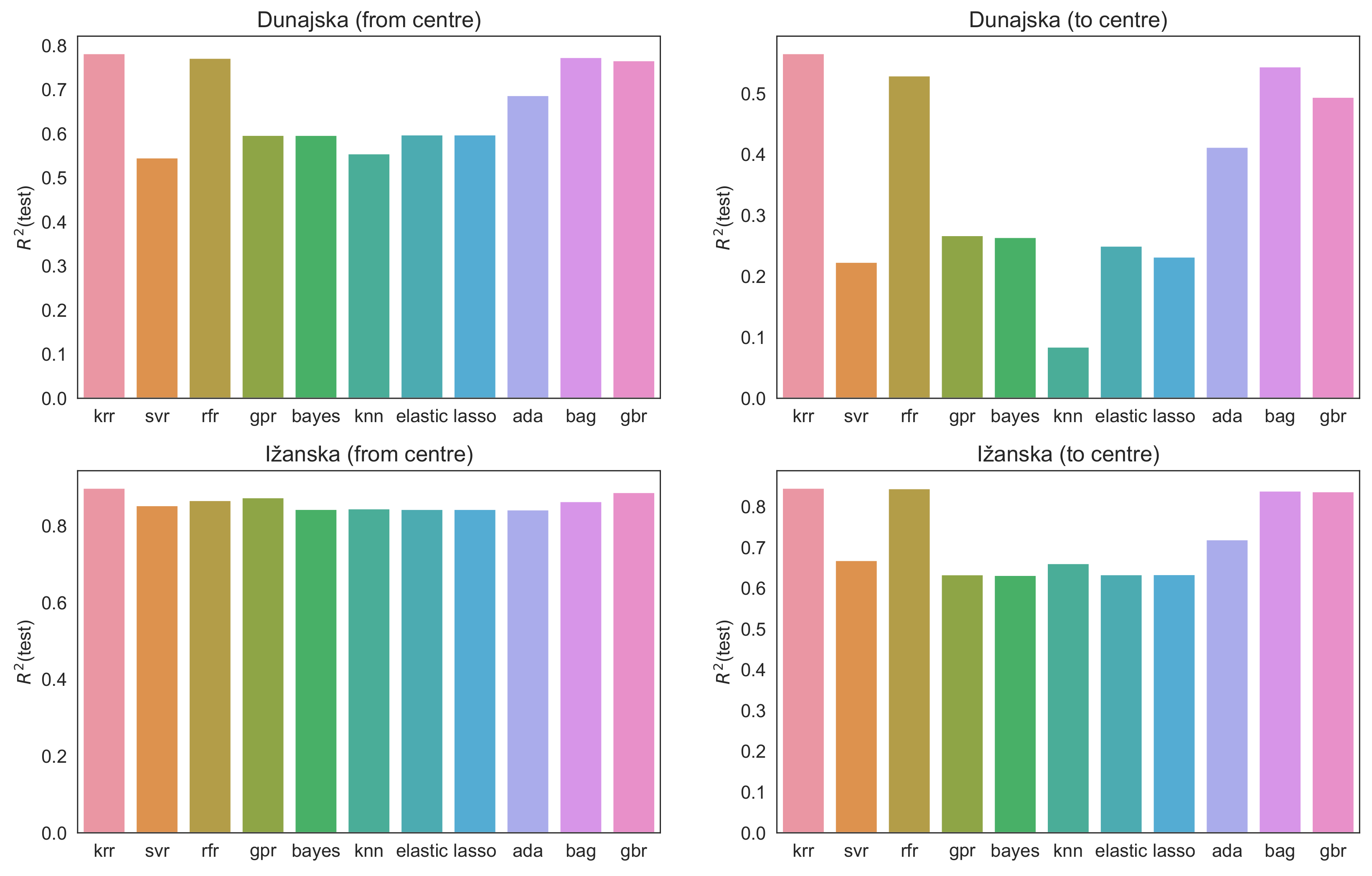
4.3. Optimal Regression Models Are Consistent through Different Segments

Finally, we identified the best regression model for a given segment using a similar procedure as described in Section 4.2. For each regression model and for each segment, we identified the feature set that yielded the best $R^2$ score on the testing dataset. The best performing models for each segment are presented in

Table 2. A summary of the results of the best regression model per each segment. The feature set denoted as basic presents the basic features, which incorporate time of day, weather conditions (good or bad), and type of day (workday or weekend). Other features describe the data obtained from Telraam counters. Abbreviations and symbols: krr—kernel ridge regression; gbr—gradient boosting regression; $R^2$ (train): coefficient of determination evaluated on the training dataset; $R^2$ (test): coefficient of determination evaluated on the testing dataset.

Segment	Features	Best Model	${\mathit{R}}^2$ (Train)	${\mathit{R}}^2$ (Test)
Dunajska (from centre)	basic, 0656-1, 0655-2	krr	0.803	0.782
Dunajska (to centre)	basic, 0656-2, 0655-1	krr	0.774	0.566
Ižanska (from centre)	basic, 0820-1, 1506-1	krr	0.947	0.899
Ižanska (to centre)	basic, 0820-2, 1506-2	krr	0.894	0.846
Slovenska (from centre)	basic, 0619-1	krr	0.898	0.892
Slovenska (to centre)	basic, 0619-2	krr	0.785	0.706
Škofije (towards Koper)	basic, 1092-1	gbr	0.895	0.867
Škofije (towards Trieste)	basic, 1092-2	krr	0.885	0.892

.

All possible features were selected in all of the cases. However, an additional (less reliable) Telraam counter did not have a significant contribution to the $R^2$ increase in the majority of the cases (see Figure 4). Even though the kernel ridge regression model performed the best on the majority of the segments, random forest regression, bagging, and gradient boost regression had very similar scores in most cases (see Figure 5).

A more accurate description of the best performing models together with their parameters is available at https://github.com/SusTra/TraCo/blob/master/best_models.pdf (accessed on 25 November 2021). We also provide these models in a pickle format to allow an interested user to reuse them. A brief description of how to load these models is provided in a README file of the repository supplementing this paper (please see https://github.com/SusTra/TraCo#readme, accessed on 25 November 2021).

5. Discussion and Conclusions

Traffic monitoring is still mostly based on conventional traffic sensors governed by traffic agencies. These are frequent on major roadways, but since their installation is difficult and costly, they are not present at all locations where vehicle counting is desired. Our goal in this research was to predict the vehicle counts based on data which are collected at low cost and easily accessible, and at the same time also fostering the engagement of wider audiences in data collecting and involving them in the scientific process by monitoring protocols. We developed a methodology to accurately predict the vehicle count data with inexpensive and less reliable sources, namely, Telraam counters combined with weather and time data. We showed that in places with absent reliable sensors these can be replaced with simple and low cost, although possibly less precise sensor systems.

A Telraam counter offers a simple device that can be used by citizens to monitor the traffic for different types of vehicles as well as pedestrians. However, these measurements can be inaccurate due to variety of reasons, e.g., bad placement of the camera or poor outdoor visibility. Some of these factors also affect the traffic conditions and were included in our models. We used regression analysis to evaluate relations between the observed variables and to increase the accuracy of an individual Telraam counter. Data gathered by reliable ILCs were taken as a reference point. Namely, the number of vehicles detected by an ILC in a given timeframe (i.e., within an hour) was regarded as the dependent variable. Initially, independent variables presented measurements by Telraam devices at approximately the same location as ILCs. To improve the prediction accuracy, we added additional features. These include the weather conditions (good or bad), the time of the day, and the type of the day (workday or weekend) when each measurement was collected. To disregard the specificity of a single micro-location, we included eight different road segments with an installed ILC and one or more Telraam counters.

For each analysed segment, we established several regression models which predicted the values of the dependent variable based on independent variables. We tested how well each model fits the observed data by calculating the respective coefficients of determination ($R^2$). In most cases, all models performed well and produced similar $R^2$ values (see Figure 5). This can be seen especially in segments Ižanska (from centre) and Slovenska (from centre), where all 11 models presented $R^2$ values above $0.8$, indicating a good fit. On the other hand, the models for segment Dunajska (to centre) showed substantially distinct relative performance. Overall, the best model with the highest $R^2$ was consistently the kernel ridge regression, winning in all cases but one (see Table 2). However, as evident from Figure 5, random forest regression, bagging, and gradient boost regression had a very similar scores as kernel ridge regression in most cases.

Kernel ridge regression combines ridge regression with the kernel trick. It learns a linear function in the space induced by the kernel and the data. If the kernel is not linear, this corresponds to a nonlinear function in the original space. Kernel ridge regression can reduce variance by shrinking parameter estimates, which makes it less susceptible to overfitting. It increases prediction accuracy even when dealing with noisy data. This is also evident in our study, where kernel ridge regression consistently yields the best results. Boosting algorithms train several models in sequence, each trying to improve the performance of its predecessor. Gradient boosting solves an optimisation problem, reducing a loss function by adding a weak learner at each step. Random forest consists of several simpler decision trees (weak learners), combining their results to make a better prediction. Each tree operates on a different subset of training data, so it observes different patterns. The combination of trees produces more robust predictions and often yields better results than linear regression, which is evident in our case. Bagging regression is another ensemble learning method that fits regressors on different random subsets of the training data and then aggregates their predictions. The techniques presented above help to reduce overfitting and gave good results in our study (see Figure 5). They also handle the collinear data well, e.g., a linear relation between two independent variables corresponding to counts by two Telraam devices. Unlike linear regression, the models that we used are nonparametric, i.e., they do not assume anything about the underlying distribution of the data. This is useful in vehicle count data since we cannot expect it to be normally distributed.

Additionally, we examined which independent variables contribute most to the goodness of model fit, i.e., how the inclusion of different variables increases $R^2$. The highest $R^2$ value was always achieved by considering all features (all Telraam counters, weather conditions, time of day, and type of day), as shown in Table 2. However, the impact of individual features varied drastically in some road segments (see Figure 4). In the Slovenska (from centre) segment, the Telraam counter 0619-1 alone sufficed for accurate prediction. In other cases (e.g., Slovenska (to centre) and Škofije (towards Trieste)), adding additional features to the Telraam counter significantly raised the $R^2$. Thus, our results showed that prediction by the less reliable Telraam counter can be substantially improved by including extra features relevant to traffic conditions. In addition, the analysis singled out the unreliable Telraam counters that do not contribute much to the model’s performance. For example, counter 0820-1 in segment Ižanska (from centre) predicted almost as well as both counters 0820-1 and 1506-1 or all features, but concerning only counter 1506-1 and excluding other variables yielded much lower values of $R^2$. Moreover, even in segments where each Telraam counter is highly unreliable, e.g., Dunajska segments, combining all these counters with basic features immensely increased the $R^2$.

Our analysis identified distinct characteristics of models relative to different road segments and various included features. Some of them were “well-behaved”, e.g., the Telraam counter 0619-1 in segment Slovenska (from centre) and counter 0820-1 in segment Ižanska (from centre). Both counters were sufficient to achieve good model fit with high $R^2$, attaining it even without considering other features (see Figure 4). Additionally, this was accomplished by all tested regression models (see Figure 5). This indicates that some Telraam counters are very reliable, i.e., they correlate highly with ILCs, as can be observed in Figure 3. The plots of counters 0820-1 and 0619-1 show high values of both Pearson’s and Spearman’s correlation coefficients and also homoscedastic behaviour. Telraam counters with these characteristics can be used to substitute ILCs with little or no loss in accuracy. Oppositely, few other counters exhibited poor performance, e.g., the aforementioned Telraam counters on the Dunajska segments. The regression models for the Dunajska (to centre) segment produced a wide range of $R^2$ values, yet even the best model achieved a relatively low score. Using any counter 0656-2 or 0655-1 alone resulted in extremely low $R^2$; thus, they had to be coupled with other features to yield useful predictions. Low correlation is noticed in the corresponding plots in Figure 3, showing low Pearson’s and Spearman’s correlation coefficients and high heteroscedasticity. We also observed the normalised mean absolute error (NMAE) of each Telraam counter regarding the observed ILC counter. This can be interpreted as a relative accuracy of a Telraam counter. However, the detection accuracy should be analysed together with correlation coefficients. Lower but consistent values of detection accuracy might produce better predictions than higher but inconsistent detection accuracy values. The segment Dunajska (to center) has a significantly higher detection accuracy than the segment Škofije (towards Koper). However, in the latter case, Telraam measurements are much better correlated with ILC measurements in comparison to the former, and thus a more accurate prediction can be obtained. The reduced detection accuracy of the observed segment is probably due to the higher vehicle speeds on the Škofije (towards Koper) segment, which is located on a highway exit. However, these errors seem to be consistent throughout the experiment and do not reduce the predictive power of the observed Telraam counter.

Although there is a growing belief that data collected by citizens promises to transform how we live, move, work, and think, there is also a growing demand to establish straightforward procedures to validate these data. Namely, the realisation of the potential of citizen science relies not only on the ability to extract information and to interpret massive data by deliberating data analytics, machine learning, and the ability to provide data-driven decisions and predictions [64] but also on the constant validation of the obtained data. Telraam data include inaccuracies due to different factors. These inaccuracies are also recognised and documented by Telramm developers [15]. They relate to the positioning of the camera, viewing angle of the camera, window transparency, etc. However, they also relate to road characteristics such as the number of lanes, road levelling, and the vicinity of traffic lights or crossroads, which can cause queuing on the counting point and thus poor vehicle recognition. Many of these challenges can be fixed by a suitable installation of the counters and information about the street profile. The accuracy of car detection is currently estimated to at least 85% in most scenarios if the device placement follows the basic requirements. The quality of the collected data and the potential to detect errors thus depend also on the end-user. The question, however is how much support and stimulation users receive by the scientific community to accurately set the devices, consciously track the data, and to intervene when deviations are detected. In this regard, Telraam encourages citizen users to provide additional information about their street profiles and to follow the ranking and benchmarking of their street segments. If a particular street has to absorb significantly more car traffic compared to other similar streets, then residents have an extra objective argument to enter into a dialogue with the local government and to engage in the planning process. This can also be considered as a step towards more verified data. Nevertheless, there is also a declared objective to develop a Telraam system also in terms of automatic solutions to filter out bad data and to advance the extrapolation techniques to estimate the typical traffic and relative traffic counts. In the near future, the Telraam sensor version 2 is planned to be released with redesigned hardware and software and an overhauled detection algorithm adopting artificial intelligence for increased accuracy of the traffic count data. As estimated by the developers, this would additionally improve the accuracy of detection and classification of different objects. Currently, more evident difficulties in object recognition are associated with distinguishing between cars and large vehicles and accurately distinguishing bikes versus pedestrians. Since in our study we only observe the vehicle counts and do not distinguish between the vehicle categories, this should not affect the observed accuracy. Another aspect to note is the visibility issues related to sunlight and weather conditions. During the night hours, the camera is not active. Since the counts are rescaled and reported for each full hour, the first and the last hour of counting in a day can have a very low up-time. For example, if the camera activates near sunrise at 6:50 in the morning, there is only a small portion of this full hour available for counting, and consequently, the rescaled data for this hour have a relatively large uncertainty. This can be managed by removing the count data for hours with camera up-times lower than some threshold, as also used in this study. However, if the up-time of the first and the last hour of daylight is nonetheless adequate even though the light conditions are poor, this can affect the obtained results due to low visibility. The same can happen in rare extreme weather conditions, such as heavy showers or extremely dense fog. The described situations are rather rare or well expected (recurrent) and thus can be managed by removing such data. Moreover, the Telraam community is planning to develop and apply a sensor that will be capable of traffic counting even in dark conditions, which will solve the above issues.

One of the contributions of this paper also includes the introduction of a methodology that can be used to validate emergent, less reliable datasources (i.e., Telraam counters) using a well-established platform (i.e., ILCs). Using the proposed methodology, we identified the anomalies in the data and tried to find the reasons for these by gaining information of the actual positions of cameras and the characteristics of a road section to acquire wider understanding of the traffic records gathered by Telraam sensors.

Another issue to be addressed here regarding the open data used in this study is in finding the reasons for the possible cut outs of counting for shorter or longer periods, due to technical problems or the subjective decision of a participant citizen to start/stop using the sensor and contributing data. While in the case of ILCs, their location and operation is constant and provides frequent and regular data, the Telraams sensors, their number, their location, and their periods of operation cannot be well predicted. Broader use of these sensors by citizens would to some extent solve this problem, as possible cut-outs could be replaced by redundant sensors in a direct vicinity. At the time of this study, the distribution of Telraam counters was still relatively sparse which limited possibilities of including more sensors per one location (road segment) in the study. Furthermore, matching the ILCs and the Telraam sensors required some compromised decisions regarding the sensors vicinity and location. We were not always able to find a micro-location with fully overlapping matches. This might not represent a large drawback when the road segment is homogeneous and not subject to major inflows or outflows between two or more counters. However, in the case of the Dunajska (to centre) segment, we recognised a significant inflow/outflow between ILC (1004-136-1) and Telraam (0655-1) counters, which might be the cause of a poor correlation between them.

Overall, the reported regression analysis showed that conventional traffic monitoring systems can be to a large degree substituted with emergent, affordable, and citized-based distributed solutions. We demonstrated this in a case study applying ILCs as current and Telraam counters as a potential future platform. One of the main benefits of the latter is also in its scalability. Namely, the number of Telraam counters can be easily increased on a given (relevant) road segment by simply engaging the general public. This also enhances the participatory role of the citizens and their concerns about their living spaces. In our opinion, increasing the number of Telraam counters to achieve a certain degree of redundancy would be able to reach or even supersede the accuracy of conventional traffic monitoring infrastructure. Using a large number of less reliable sensors to improve the accuracy of obtained data has already been successfully employed in different engineering disciplines [65]. An example vividly illustrating the concept of improving the measurement accuracy by redundancy was reported by Weiss et al., who presented a highly accurate clock implemented with the integration of data obtained by using a set of inexpensive and imprecise watches [66]. In our case, we were able to obtain relatively accurate predictions of count data by employing a single or two Telraam counters. We believe that increasing their numbers would additionally improve the prediction accuracy and would thus provide a reliable infrastructure for traffic monitoring. In the near future, this infrastructure could as well be supplemented with alternative citizen-engaged projects and initiatives directed towards planning and maintaining sustainable cities.

References

1. Zhao, P.; Hu, H. Geographical patterns of traffic congestion in growing megacities: Big data analytics from Beijing. Cities 2019, 92, 164–174. [Google Scholar] [CrossRef]
2. Buzási, A.; Csete, M. Sustainability indicators in assessing urban transport systems. Period. Polytech. Transp. Eng. 2015, 43, 138–145. [Google Scholar] [CrossRef] [Green Version]
3. Lin, Y.; Benneker, K. Assessing collaborative planning and the added value of planning support apps in The Netherlands. Environ. Plan. B Urban Anal. City Sci. 2021. [Google Scholar] [CrossRef]
4. Offenhuber, D.; Ratti, C. Decoding the City; Birkhäuser: Basel, Switzerland, 2014. [Google Scholar]
5. Becken, S.; Connolly, R.M.; Chen, J.; Stantic, B. A hybrid is born: Integrating collective sensing, citizen science and professional monitoring of the environment. Ecol. Inform. 2019, 52, 35–45. [Google Scholar] [CrossRef]
6. Welvaert, M.; Caley, P. Citizen surveillance for environmental monitoring: Combining the efforts of citizen science and crowdsourcing in a quantitative data framework. SpringerPlus 2016, 5, 1–14. [Google Scholar] [CrossRef] [Green Version]
7. Coulson, S.; Woods, M. Citizen Sensing: An action-orientated framework for citizen science. Front. Commun. 2021, 6, 629700. [Google Scholar] [CrossRef]
8. Eitzel, M.V.; Cappadonna, J.L.; Santos-Lang, C.; Duerr, R.E.; Virapongse, A.; West, S.E.; Kyba, C.; Bowser, A.; Cooper, C.B.; Sforzi, A.; et al. Citizen science terminology matters: Exploring key terms. Citiz. Sci. Theory Pract. 2017, 2, 1. [Google Scholar] [CrossRef] [Green Version]
9. Riesch, H.; Potter, C. Citizen science as seen by scientists: Methodological, epistemological and ethical dimensions. Public Underst. Sci. 2014, 23, 107–120. [Google Scholar] [CrossRef]
10. Boulos, M.N.K.; Resch, B.; Crowley, D.N.; Breslin, J.G.; Sohn, G.; Burtner, R.; Pike, W.A.; Jezierski, E.; Chuang, K.Y.S. Crowdsourcing, citizen sensing and sensor web technologies for public and environmental health surveillance and crisis management: Trends, OGC standards and application examples. Int. J. Health Geogr. 2011, 10, 1–29. [Google Scholar]
11. Kosmala, M.; Wiggins, A.; Swanson, A.; Simmons, B. Assessing data quality in citizen science. Front. Ecol. Environ. 2016, 14, 551–560. [Google Scholar] [CrossRef] [Green Version]
12. Uhlmann, E.L.; Ebersole, C.R.; Chartier, C.R.; Errington, T.M.; Kidwell, M.C.; Lai, C.K.; McCarthy, R.J.; Riegelman, A.; Silberzahn, R.; Nosek, B.A. Scientific utopia III: Crowdsourcing science. Perspect. Psychol. Sci. 2019, 14, 711–733. [Google Scholar] [CrossRef] [Green Version]
13. Lodi, L.; Tardin, R. Citizen science contributes to the understanding of the occurrence and distribution of cetaceans in southeastern Brazil—A case study. Ocean Coast. Manag. 2018, 158, 45–55. [Google Scholar] [CrossRef]
14. Ekman, K.; Weilenmann, A. Behind the scenes of planning for public participation: Planning for air-quality monitoring with low-cost sensors. J. Environ. Plan. Manag. 2021, 64, 865–882. [Google Scholar] [CrossRef]
15. Telraam. Available online: https://telraam.net/ (accessed on 25 November 2021).
16. Elfar, A.; Talebpour, A.; Mahmassani, H.S. Machine learning approach to short-term traffic congestion prediction in a connected environment. Transp. Res. Rec. 2018, 2672, 185–195. [Google Scholar] [CrossRef]
17. Büchel, B.; Corman, F. Review on Statistical Modeling of Travel Time Variability for Road-Based Public Transport. Front. Built Environ. 2020, 6, 70. [Google Scholar] [CrossRef]
18. Altintasi, O.; Tuydes-Yaman, H.; Tuncay, K. Detection of urban traffic patterns from Floating Car Data (FCD). Transp. Res. Procedia 2017, 22, 382–391. [Google Scholar] [CrossRef]
19. Tasgaonkar, P.P.; Garg, R.D.; Garg, P.K. Vehicle detection and traffic estimation with sensors technologies for intelligent transportation systems. Sens. Imaging 2020, 21, 1–28. [Google Scholar] [CrossRef]
20. Jain, N.K.; Saini, R.; Mittal, P. A review on traffic monitoring system techniques. In Soft Computing: Theories and Applications; Springer: Singapore, 2019; pp. 569–577. [Google Scholar]
21. Middleton, D.R.; Parker, R.; Longmire, R. Investigation of Vehicle Detector Performance and ATMS Interface; Technical Report; Texas Transportation Institute, Texas A & M University System: College Station, TX, USA, 2007. [Google Scholar]
22. Bellucci, P.; Cipriani, E. Data accuracy on automatic traffic counting: The SMART project results. Eur. Transp. Res. Rev. 2010, 2, 175–187. [Google Scholar] [CrossRef] [Green Version]
23. Federal Highway Administration. Traffic Monitoring Guide; Technical Report; U.S. Department of Transportation: Washington, DC, USA, 2016. [Google Scholar]
24. Klein, L.A.; Mills, M.K.; Gibson, D.R. Traffic Detector Handbook: Volume I; Technical Report; Turner-Fairbank Highway Research Center: McLean, VA, USA, 2006. [Google Scholar]
25. Holmgren, J.; Fredriksson, H.; Dahl, M. Traffic data collection using active mobile and stationary devices. Procedia Comput. Sci. 2020, 177, 49–56. [Google Scholar] [CrossRef]
26. Ahmadi, S.A.; Ghorbanian, A.; Mohammadzadeh, A. Moving vehicle detection, tracking and traffic parameter estimation from a satellite video: A perspective on a smarter city. Int. J. Remote Sens. 2019, 40, 8379–8394. [Google Scholar] [CrossRef]
27. Lesani, A.; Nateghinia, E.; Miranda-Moreno, L.F. Development and evaluation of a real-time pedestrian counting system for high-volume conditions based on 2D LiDAR. Transp. Res. Part C Emerg. Technol. 2020, 114, 20–35. [Google Scholar] [CrossRef]
28. Astarita, V.; Giofrè, V.P.; Guido, G.; Vitale, A. A review of traffic signal control methods and experiments based on Floating Car Data (FCD). Procedia Comput. Sci. 2020, 175, 745–751. [Google Scholar] [CrossRef]
29. Ghahramani, M.; Zhou, M.; Wang, G. Urban sensing based on mobile phone data: Approaches, applications, and challenges. IEEE/CAA J. Autom. Sin. 2020, 7, 627–637. [Google Scholar] [CrossRef]
30. Alkouz, B.; Al Aghbari, Z. SNSJam: Road traffic analysis and prediction by fusing data from multiple social networks. Inf. Process. Manag. 2020, 57, 102139. [Google Scholar] [CrossRef]
31. Nikolaidou, A.; Papaioannou, P. Utilizing social media in transport planning and public transit quality: Survey of literature. J. Transp. Eng. Part A Syst. 2018, 144, 04018007. [Google Scholar] [CrossRef]
32. Trivedi, J.D.; Mandalapu, S.D.; Dave, D.H. Vision-based Real-time Vehicle Detection and Vehicle Speed Measurement using morphology and binary logical operation. J. Ind. Inf. Integr. 2021, 100280. [Google Scholar] [CrossRef]
33. Datondji, S.R.E.; Dupuis, Y.; Subirats, P.; Vasseur, P. A survey of vision-based traffic monitoring of road intersections. IEEE Trans. Intell. Transp. Syst. 2016, 17, 2681–2698. [Google Scholar] [CrossRef]
34. Unzueta, L.; Nieto, M.; Cortés, A.; Barandiaran, J.; Otaegui, O.; Sánchez, P. Adaptive multicue background subtraction for robust vehicle counting and classification. IEEE Trans. Intell. Transp. Syst. 2011, 13, 527–540. [Google Scholar] [CrossRef]
35. Badino, H.; Franke, U.; Mester, R. Free Space Computation Using Stochastic Occupancy Grids and Dynamic Programming. In Proceedings of the Workshop on Dynamical Vision, ICCV, Rio de Janeiro, Brazil, 14–21 October 2007; Volume 20. [Google Scholar]
36. Zhu, Y.; Comaniciu, D.; Pellkofer, M.; Koehler, T. Reliable detection of overtaking vehicles using robust information fusion. IEEE Trans. Intell. Transp. Syst. 2006, 7, 401–414. [Google Scholar] [CrossRef]
37. Zhou, J.; Gao, D.; Zhang, D. Moving vehicle detection for automatic traffic monitoring. IEEE Trans. Veh. Technol. 2007, 56, 51–59. [Google Scholar] [CrossRef] [Green Version]
38. Zhao, Z.Q.; Zheng, P.; Xu, S.t.; Wu, X. Object detection with deep learning: A review. IEEE Trans. Neural Netw. Learn. Syst. 2019, 30, 3212–3232. [Google Scholar] [CrossRef] [PubMed] [Green Version]
39. Wang, H.; Yu, Y.; Cai, Y.; Chen, X.; Chen, L.; Liu, Q. A comparative study of state-of-the-art deep learning algorithms for vehicle detection. IEEE Intell. Transp. Syst. Mag. 2019, 11, 82–95. [Google Scholar] [CrossRef]
40. Song, H.; Liang, H.; Li, H.; Dai, Z.; Yun, X. Vision-based vehicle detection and counting system using deep learning in highway scenes. Eur. Transp. Res. Rev. 2019, 11, 1–16. [Google Scholar] [CrossRef] [Green Version]
41. O’Mahony, N.; Campbell, S.; Carvalho, A.; Harapanahalli, S.; Hernandez, G.V.; Krpalkova, L.; Riordan, D.; Walsh, J. Deep learning vs. traditional computer vision. In Science and Information Conference; Springer: Cham, Switzerland, 2019; pp. 128–144. [Google Scholar]
42. Yang, H.; Zhang, Y.; Zhang, Y.; Meng, H.; Li, S.; Dai, X. A Fast Vehicle Counting and Traffic Volume Estimation Method Based on Convolutional Neural Network. IEEE Access 2021, 9, 150522–150531. [Google Scholar] [CrossRef]
43. Wang, Y.; Ban, X.; Wang, H.; Wu, D.; Wang, H.; Yang, S.; Liu, S.; Lai, J. Detection and classification of moving vehicle from video using multiple spatio-temporal features. IEEE Access 2019, 7, 80287–80299. [Google Scholar] [CrossRef]
44. Zhang, X.; Gao, H.; Xue, C.; Zhao, J.; Liu, Y. Real-time vehicle detection and tracking using improved histogram of gradient features and Kalman filters. Int. J. Adv. Robot. Syst. 2018, 15, 1729881417749949. [Google Scholar] [CrossRef]
45. Azimjonov, J.; Özmen, A. A real-time vehicle detection and a novel vehicle tracking systems for estimating and monitoring traffic flow on highways. Adv. Eng. Inform. 2021, 50, 101393. [Google Scholar] [CrossRef]
46. Meng, F.; Wong, S.C.; Wong, W.; Li, Y. Estimation of scaling factors for traffic counts based on stationary and mobile sources of data. Int. J. Intell. Transp. Syst. Res. 2017, 15, 180–191. [Google Scholar] [CrossRef] [Green Version]
47. Tavasszy, L.; De Jong, G. Modelling Freight Transport; Elsevier: Amsterdam, The Netherlands, 2013. [Google Scholar]
48. Den Broeder, L.; Lemmens, L.; Uysal, S.; Kauw, K.; Weekenborg, J.; Schönenberger, M.; Klooster-Kwakkelstein, S.; Schoenmakers, M.; Scharwächter, W.; Van de Weerd, A.; et al. Public health citizen science; perceived impacts on citizen scientists: A case study in a low-income neighbourhood in the Netherlands. Citiz. Sci. Theory Pract. 2017, 2, 7. [Google Scholar] [CrossRef] [Green Version]
49. Aoki, P.; Woodruff, A.; Yellapragada, B.; Willett, W. Environmental protection and agency: Motivations, capacity, and goals in participatory sensing. In Proceedings of the 2017 CHI Conference on Human Factors in Computing Systems, Denver, CO, USA, 6–11 May 2017; pp. 3138–3150. [Google Scholar]
50. Bria, F.; Gascó, M.; Kresin, F. Growing a Digital Social Innovation Ecosystem for Europe; Technical Report; European Commission: Brussels, Belgium, 2015. [Google Scholar]
51. Visual Crossing Weather History API. Available online: https://www.visualcrossing.com/weather-api (accessed on 15 November 2021).
52. Vovk, V. Kernel ridge regression. In Empirical Inference; Springer: Berlin/Heidelberg, Germany, 2013; pp. 105–116. [Google Scholar]
53. Awad, M.; Khanna, R. Support vector regression. In Efficient Learning Machines; Springer: Berlin/Heidelberg, Germany, 2015; pp. 67–80. [Google Scholar]
54. Segal, M. Machine Learning Benchmarks and Random Forest Regression; Technical Report; Center for Bioinformatics & Molecular Biostatistics, University of California: San Francisco, CA, USA, 2003. [Google Scholar]
55. Schulz, E.; Speekenbrink, M.; Krause, A. A tutorial on Gaussian process regression: Modelling, exploring, and exploiting functions. J. Math. Psychol. 2018, 85, 1–16. [Google Scholar] [CrossRef]
56. Shi, Q.; Abdel-Aty, M.; Lee, J. A Bayesian ridge regression analysis of congestion’s impact on urban expressway safety. Accid. Anal. Prev. 2016, 88, 124–137. [Google Scholar] [CrossRef] [PubMed]
57. Maltamo, M.; Kangas, A. Methods based on k-nearest neighbor regression in the prediction of basal area diameter distribution. Can. J. For. Res. 1998, 28, 1107–1115. [Google Scholar] [CrossRef]
58. Zou, H.; Hastie, T. Regularization and variable selection via the elastic net. J. R. Stat. Soc. Ser. B (Stat. Methodol.) 2005, 67, 301–320. [Google Scholar] [CrossRef] [Green Version]
59. Ranstam, J.; Cook, J. LASSO regression. J. Br. Surg. 2018, 105, 1348. [Google Scholar] [CrossRef]
60. Schapire, R.E. Explaining adaboost. In Empirical Inference; Springer: Berlin/Heidelberg, Germany, 2013; pp. 37–52. [Google Scholar]
61. Quinlan, J.R. Bagging, boosting, and C4. 5. In Proceedings of the Thirteenth National Conference on Artificial Intelligence (AAAI-96), Portland, OR, USA, 4–8 August 1996; pp. 725–730. [Google Scholar]
62. Zhang, Y.; Haghani, A. A gradient boosting method to improve travel time prediction. Transp. Res. Part C Emerg. Technol. 2015, 58, 308–324. [Google Scholar] [CrossRef]
63. Pedregosa, F.; Varoquaux, G.; Gramfort, A.; Michel, V.; Thirion, B.; Grisel, O.; Blondel, M.; Prettenhofer, P.; Weiss, R.; Dubourg, V.; et al. Scikit-learn: Machine Learning in Python. J. Mach. Learn. Res. 2011, 12, 2825–2830. [Google Scholar]
64. Balázs, B.; Mooney, P.; Nováková, E.; Bastin, L.; Arsanjani, J.J. Data quality in citizen science. In The Science of Citizen Science; Springer: Cham, Switzerland, 2021; p. 139. [Google Scholar]
65. Jafari, M. Optimal redundant sensor configuration for accuracy increasing in space inertial navigation system. Aerosp. Sci. Technol. 2015, 47, 467–472. [Google Scholar] [CrossRef] [Green Version]
66. Weiss, M.; Allan, D.; Davis, D.; Levine, J. Smart clock: A new time. IEEE Trans. Instrum. Meas. 1992, 41, 915–918. [Google Scholar] [CrossRef]
Figure 1. Distributions of data obtained with Telraam counters.
Sustainability 14 00622 g001
Figure 2. Distributions of data obtained with inductive loop counters.
Sustainability 14 00622 g002
Figure 3. Correlations between inductive loop counters (y axes) and Telraam counters (x axes). Different colours indicate different road segments. Symbols and abbreviations: r P —Pearson’s correlation coefficient; r S —Spearman’s correlation coefficient; N M A E —normalised mean absolute error.
Sustainability 14 00622 g003
Figure 4. Dependence of R 2 of a testing dataset on the feature set included in a regression model. Each subplot presents the results obtained on a selected road segment. The feature set denoted as basic presents the basic features, which incorporate time of day, weather conditions (good or bad), and type of a day (workday or weekend). Other features describe the data obtained from Telraam counters. The results obtained with the best regression model for a given scenario are presented. Different colours indicate different feature sets.
Sustainability 14 00622 g004
Figure 5. Dependence of R 2 of a testing dataset on a regression model. Each subplot presents the results obtained on a selected road segment. The results obtained with the best feature set for a given scenario are presented. Different colours indicate different regression models. Abbreviations and symbols: krr—kernel ridge regression; svr—support vector regression; rfr—random forest regression; gpr—Gaussian process regression; bayes—Bayesian ridge regression; knn—K-nearest neighbours regression; elastic—elastic net regression; lasso—LASSO regression; ada—AdaBoost regression; bag—bagging regression; gbr—gradient boosting regression.
Sustainability 14 00622 g005aSustainability 14 00622 g005b