Analysis of Driving Control Characteristics in Typical Road Types
Abstract
:1. Introduction
- (1)
- An experiment is designed in a closed test site to build a naturalistic dataset which contains both vehicle running state parameters collected from typical road types and interaction behaviors between vehicles.
- (2)
- Taking the driving control parameters in a long straight road as the control group, multiple vehicle running parameters and their derivative indices undergo a cross-analysis to show the driving control characteristics in different road types.
- (3)
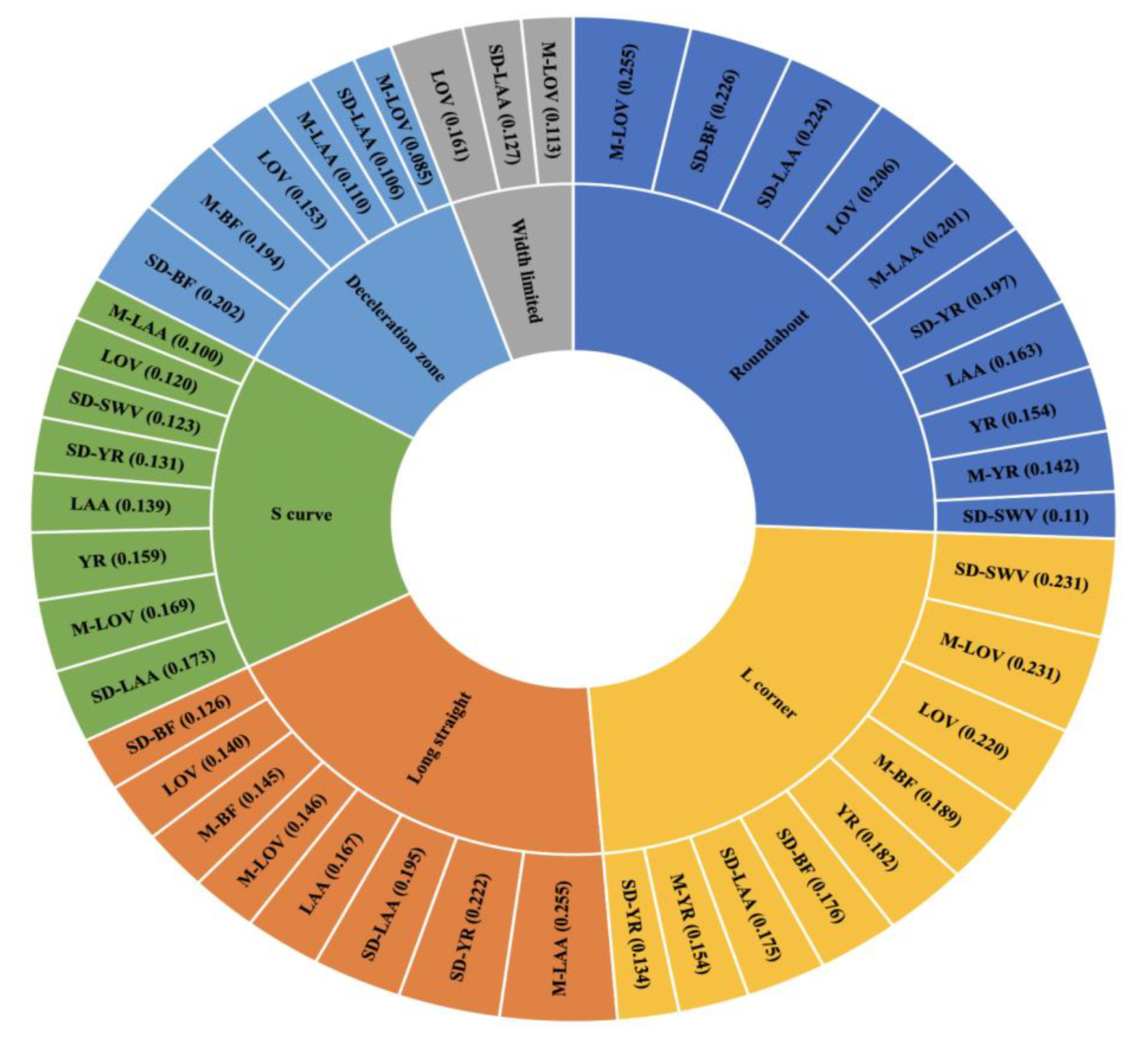
- After weighing the indices in each road types, the differentiated indices of driving control characteristics in each scene can be obtained. Finally, the results of the driving control characteristics in different road types are analyzed and discussed.
2. Experiment and Dataset
2.1. Subjects
2.2. Experiment Site
2.3. Experiment Design
- (a)
- The driver was strictly required to follow the lane line and not to press the line. The driving task for each road segment had to be completed; otherwise, the driver was required to start again.
- (b)
- The driver was required to pay full attention without engaging in any secondary tasks, such as talking or making phone calls. No drug or alcohol effects were observed.
- (c)
- Each time the experiment was repeated, the starting and ending points of the vehicle had to correspond to the setting lines strictly.
2.4. Establishment of Dataset
- (a)
- Longitudinal velocity (LOV): Velocity in the direction of the vehicle.
- (b)
- Longitudinal acceleration (LOA): Acceleration in the direction of the vehicle.
- (c)
- Braking force (BF): Real-time pressure value of the brake pedal.
- (d)
- Yaw rate (YR): The deflection of a car about the vertical axis.
- (e)
- Steering wheel angle velocity (SWV): Ratio of steering wheel angle difference to sampling time interval between adjacent sampling points.
- (f)
- Lateral acceleration (LAA): Acceleration perpendicular to the direction of the car.
3. Driving Control Characteristic Evaluation Indices
3.1. Entropy Weight Method
- Step 1. Standardized evaluation matrix.
- Step 2. Characteristic proportion of indices.
- Step 3. Information entropy of the indices.
- Step 4. Weight calculation based on information entropy redundancy.
3.2. Technique for Order Preference by Similarity to an Ideal Solution
- Step 1. The intermediate positive processing of indices
- Step 2. Construction of normalized initial matrix
- Step 3. Distance calculation between indices in other scenes and the long straight scene.
3.3. Weight and Distance Calculation of Characteristic Evaluation Indices in Typical Road Types
3.4. Longitudinal Parameters
3.4.1. Longitudinal Velocity
- (a)
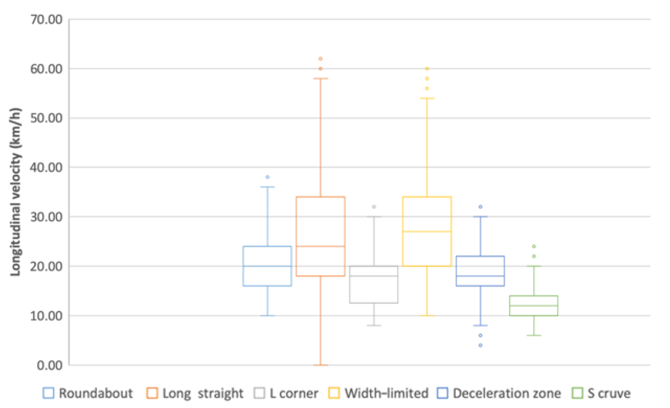
- From the box plot (Figure 5), the distribution of LOV values in each scene is different.
- (b)
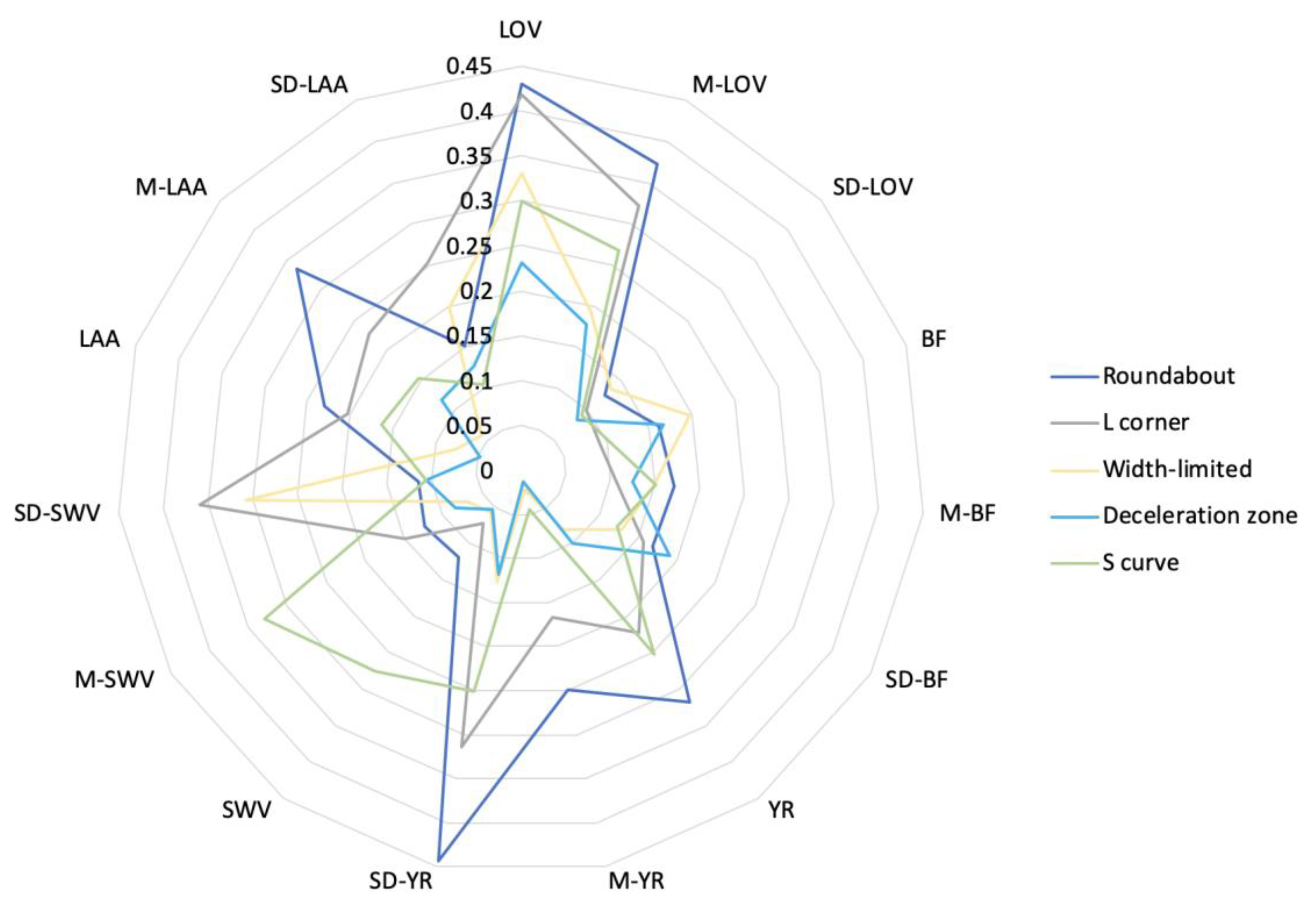
- From the radar chart (Figure 4), the LOV in other scenes is far away from that in the long straight scene, and there is no close coincidence among them. This is in line with the result of (a).
- (c)
- From the ANOVA (Table 3), it can be seen that in different scenes, the difference of LOV in every scene is extremely significant, which is in line with the result of (a) and (b).
- (d)
- Summary: LOV shows significant differences in each scene and can be used to represent the driving control characteristics in six scenes.
3.4.2. Mean of Longitudinal Velocity
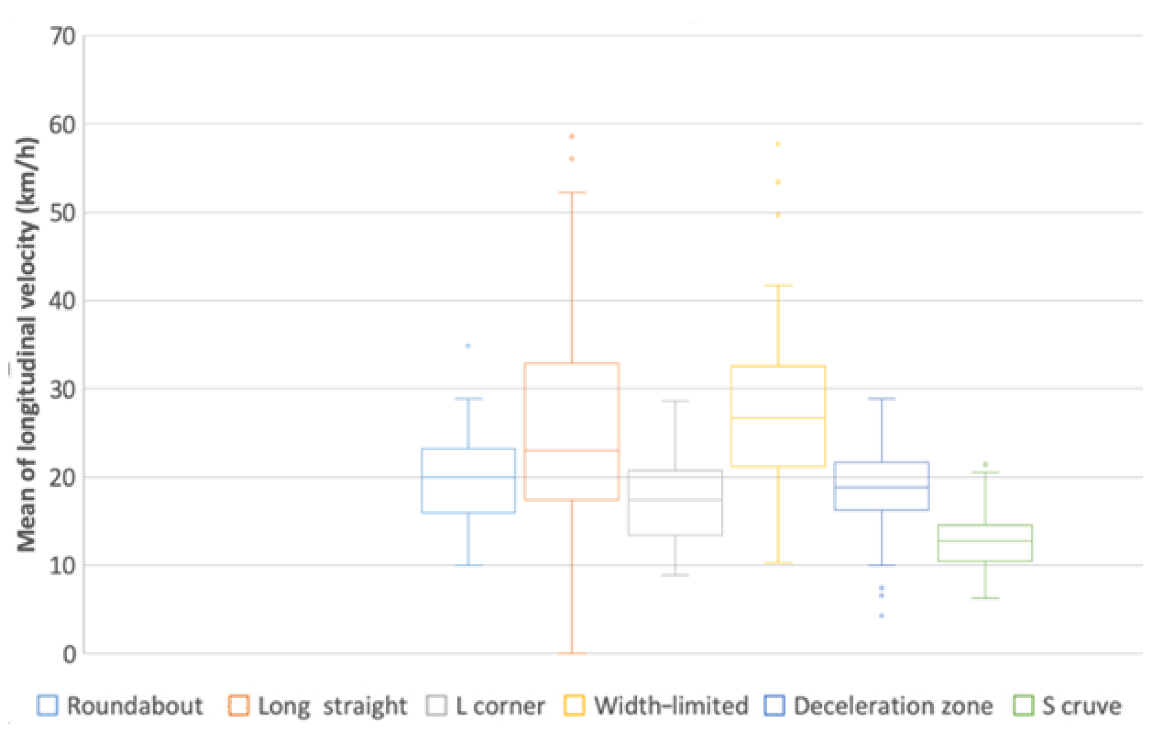
- (a)
- From the box plot (Figure 6), the distribution of M-LOV values in each scene is different.
- (b)
- From the radar chart (Figure 4), the M-LOV values in other scenes are far away from that in the long straight scene. This is in line with the result of (a).
- (c)
- From the ANOVA (Table 4), it can be seen that in different scenes, the differences of LOV in every scene are extremely significant, which is in line with the result of (a) and (b).
- (d)
- Summary: M-LOV shows significant differences in each scene and can be used to represent the driving control characteristics in six scenes.
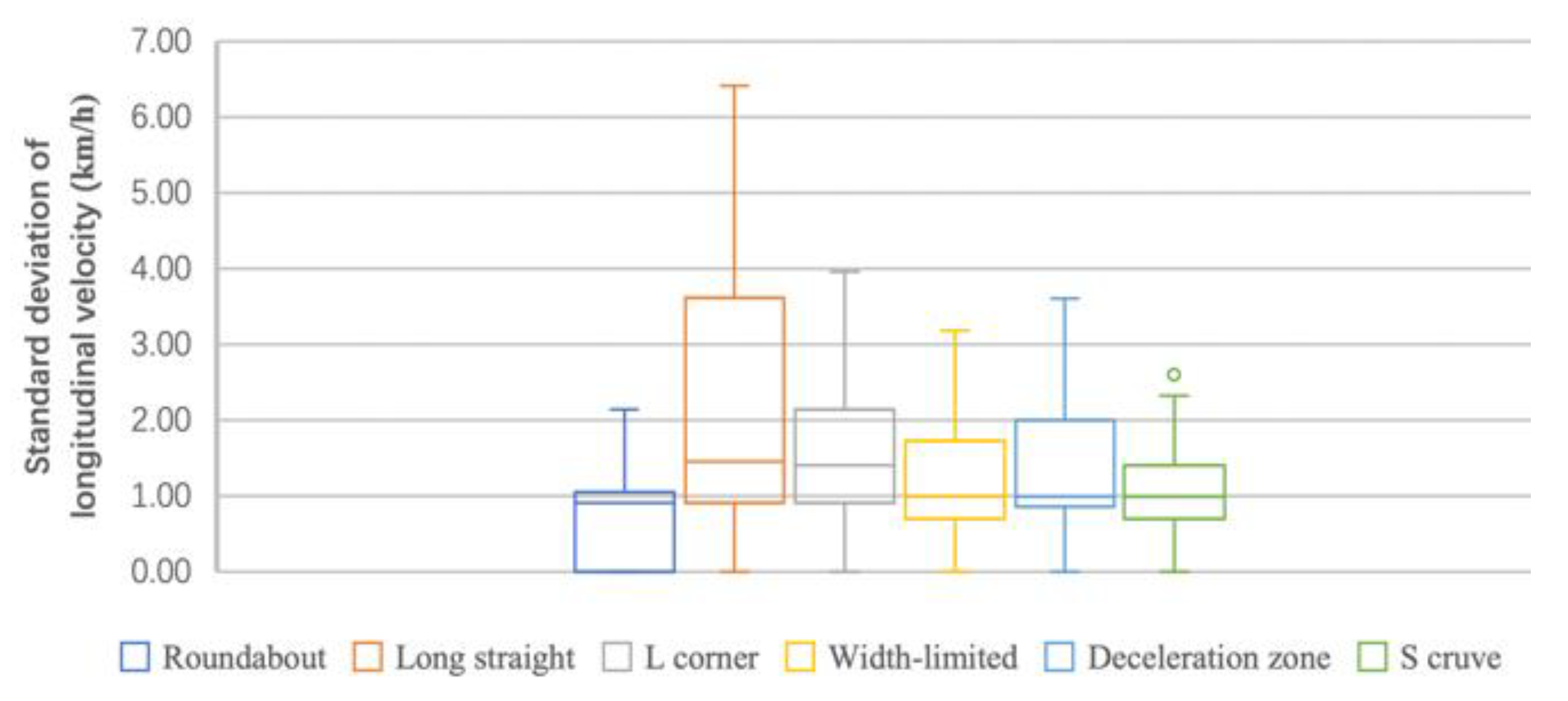
3.4.3. Standard Deviation of Longitudinal Velocity
- (a)
- From the box plot (Figure 7), the distribution of SD-LOV values in width-limited and deceleration scenes are similar, and the rest are different from each other.
- (b)
- From the radar chart (Figure 4), the SD-LOV values in other scenes are far away from that in the long straight scene.
- (c)
- From the ANOVA (Table 5), it can be seen that in different scenes, the differences of SD-LOV in every scene are extremely significant, which is in line with the result of (a) and (b).
- (d)
- Summary: The results of (a), (b) and (c) cannot be consistent; thus, the SD-LOV does not meet the requirements.
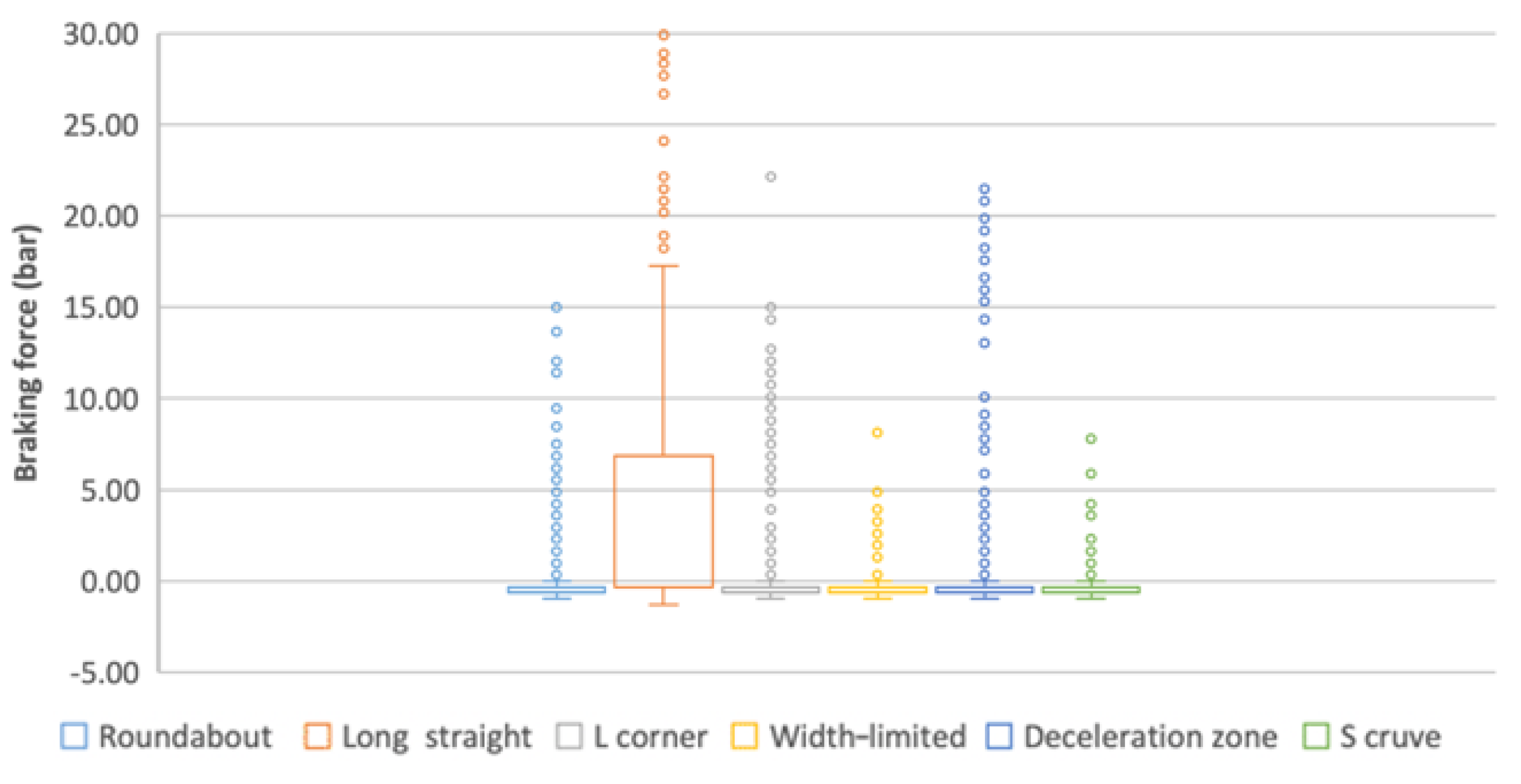
3.4.4. Braking Force
- (a)
- From the box plot (Figure 8), the distribution of BF values is analogous between roundabout and L-corner, S-curve and width-limited.
- (b)
- From the radar chart (Figure 4), the BF values in other scenes are far away from that in the long straight scene, which in line with (c). However, roundabout and deceleration zone, as well as L-corner and S-curve, almost coincide.
- (c)
- From the ANOVA (Table 6), there are significant differences in BF between other scenes and the long straight scene.
- (d)
- Summary: Although (b) and (c) reflect the coincident differences among indices, the results of (a) and (b) indicate that there may be multiple collinearity problems between each index, so that BF cannot be used to represent the respective characteristics of scene indices.
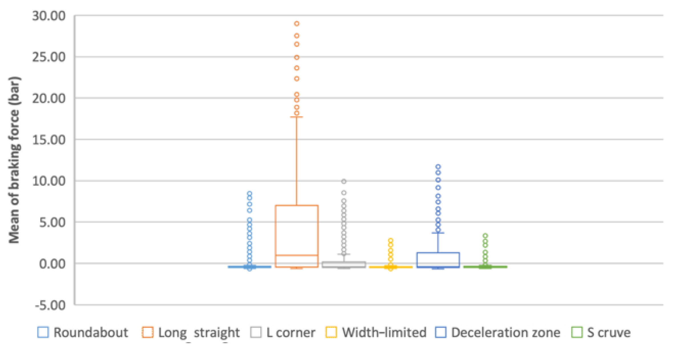
3.4.5. Mean of Braking Force
- (a)
- From the box plot (Figure 9), the distribution of M-BF values is analogous between width-limited and S-curve, while the distribution of others is varied.
- (b)
- From the radar chart (Figure 4), the M-BF values in other scenes are far away from that in the long straight scene, and the distance of width-limited coincides with that of S-curve, which is in line with the result of (a) and (c).
- (c)
- From the ANOVA (Table 7), there are significant differences in M-BF between other scenes and the long straight scene.
- (d)
- Summary: M-BF can be used to represent the driving control characteristic in driving scenes including long straight, roundabout, L-corner and deceleration zone.
3.4.6. Standard Deviation of Braking Force
- (a)
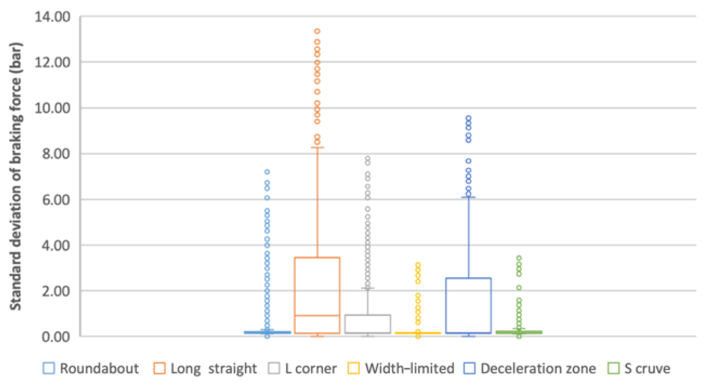
- From the box plot (Figure 10), the distribution of SD-BF values is analogous between width-limited and S-curve, while the distribution of others is varied.
- (b)
- From the radar chart (Figure 4), the SD-BF values in each scene are far from that in the long straight scene, and the distance of width-limited coincides with that of S-curve, which is in line with the results of a) and c).
- (c)
- From the ANOVA (Table 8), significant differences appear in SD-BF between other scenes and the long straight scene.
- (d)
- Summary: SD-BF can be used to represent the driving control characteristic in driving scenes including long straight, roundabout, L-corner and deceleration zone.
3.5. Lateral Parameters
3.5.1. Yaw Rate
- (a)
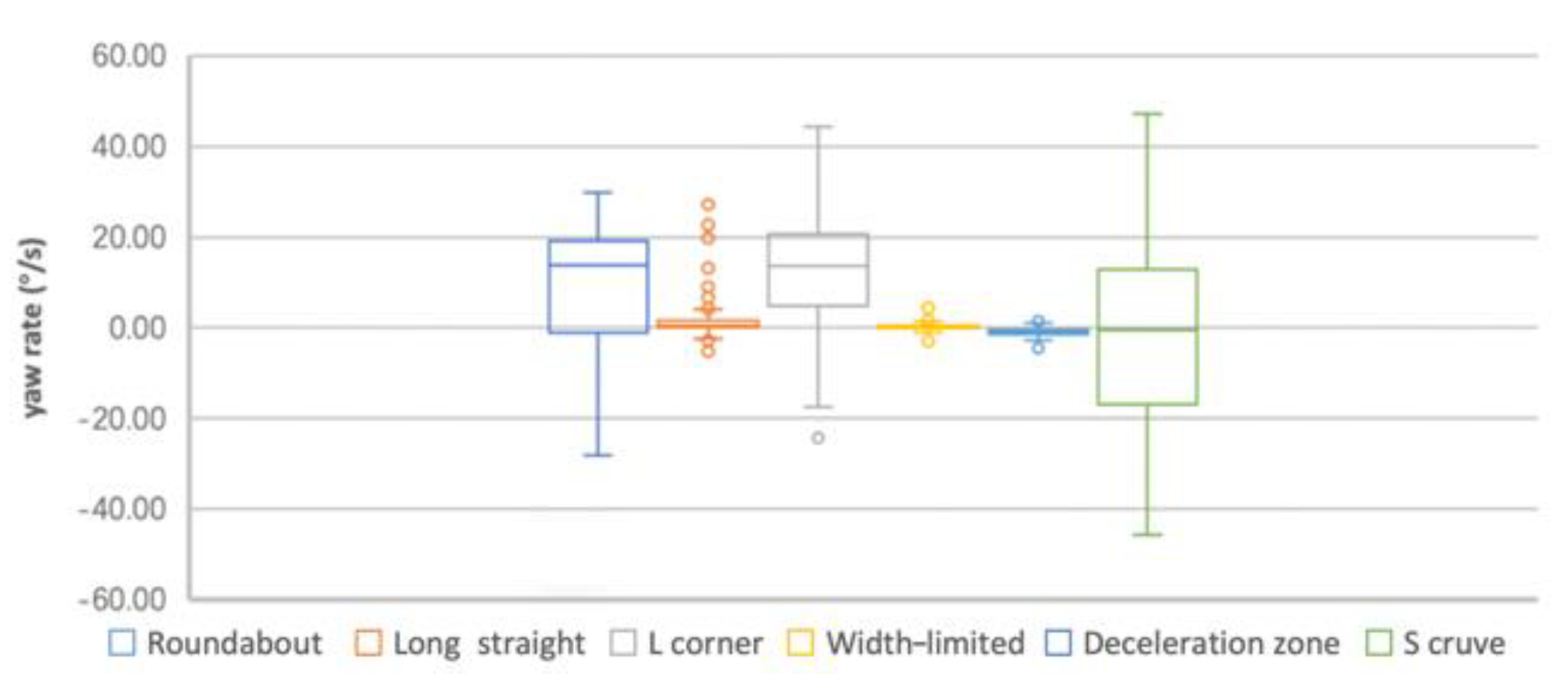
- From the box plot (Figure 11), the distribution of YR values is analogous between width-limited and deceleration zone, while the distribution of others is varied.
- (b)
- From the radar chart (Figure 4), the YR values in width-limited and deceleration zone are close to center, which means that the difference of YR among long straight, width-limited and deceleration zone is low. This is in line with the results of (a).
- (c)
- From the ANOVA (Table 9), no significant difference appears between long straight, width-limited and deceleration zone.
- (d)
- Summary: The YR shows low-level difference in long straight, width-limited and deceleration zone. Therefore, YR can be used to represent the driving control characteristic in driving scenes including S-curve, roundabout and L-corner.
3.5.2. Mean of Yaw Rate
- (a)
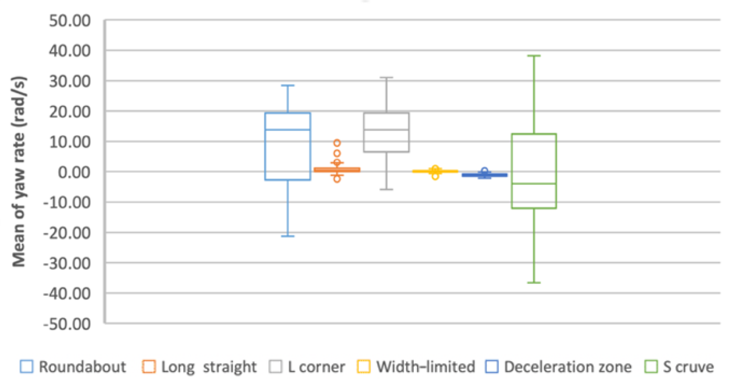
- From the box plot (Figure 12), the distribution of M-YR values is analogous between width-limited and deceleration zone, while the distribution of others is varied.
- (b)
- From the radar chart (Figure 4), the M-YR values in width-limited, S-curve and deceleration zone are close to center, which means that the difference of M-YR among long straight, S-curve, width-limited and deceleration zone is low. This is in line with the results of (a).
- (c)
- From the ANOVA (Table 10), no significant difference appears between long straight, width-limited, S-curve and deceleration zone.
- (d)
- Summary: The M-YR shows low-level difference in long straight, width-limited, S-curve and deceleration zone. Therefore, M-YR can be used to represent the driving control characteristic in driving scenes including roundabout and L-corner.
3.5.3. Standard Deviation of Yaw Rate
- (a)
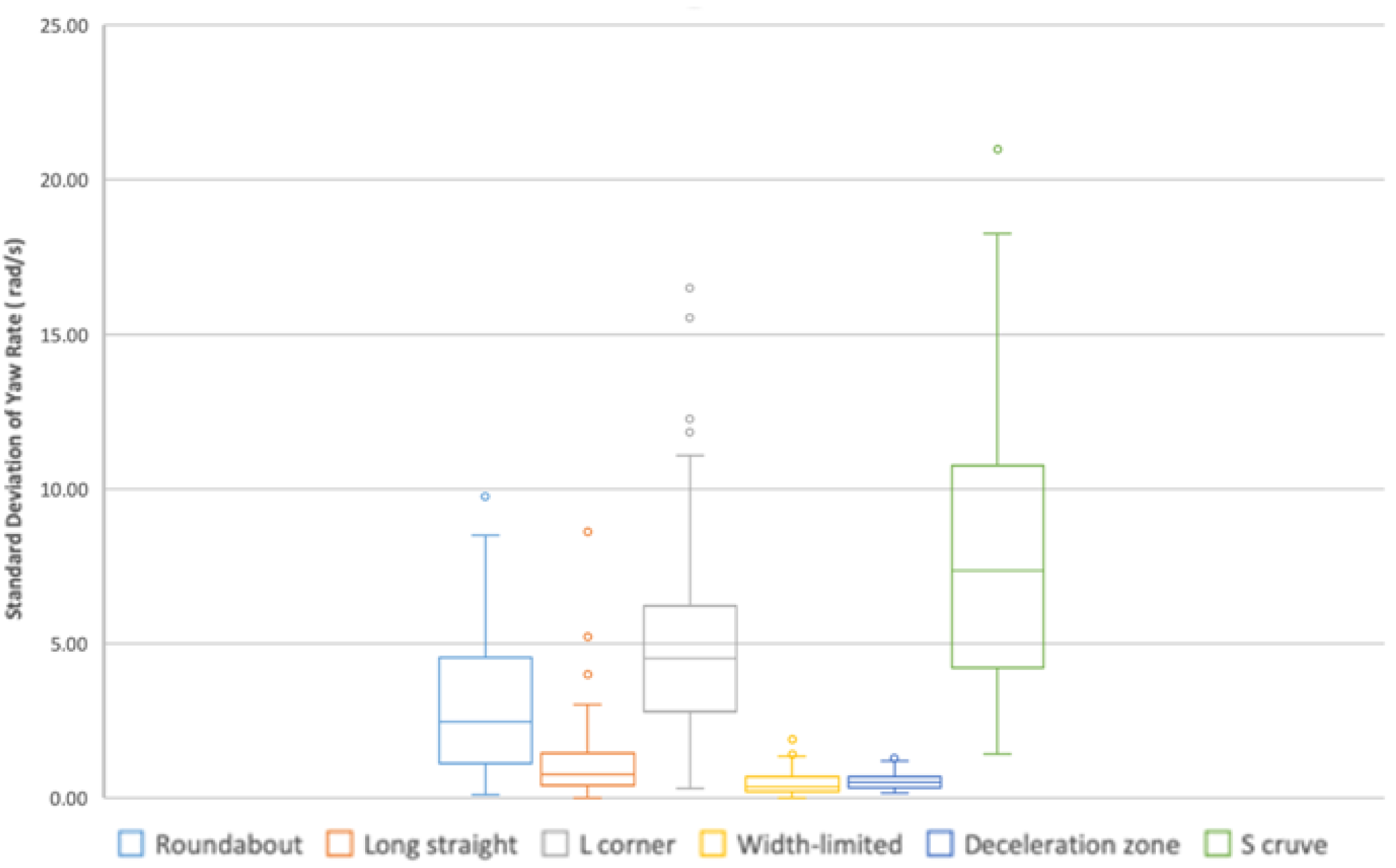
- From the box plot (Figure 13), the distribution of SD-YR values is analogous between width-limited and deceleration zone, while the distribution of others is varied.
- (b)
- From the radar chart (Figure 4), the M-YR values in all scenes are far from center, which is in line with (c). Moreover, the M-YR value in width-limited coincides with that in deceleration zone, which is in line with (a).
- (c)
- From the ANOVA (Table 11), significant differences appear in SD-YR between other scenes and the long straight scene.
- (d)
- Summary: The SD-YR can be used to represent the driving control characteristic in driving scenes including long straight, roundabout, L-corner and S-curve.
3.5.4. Steering Wheel Angle Velocity
- (a)
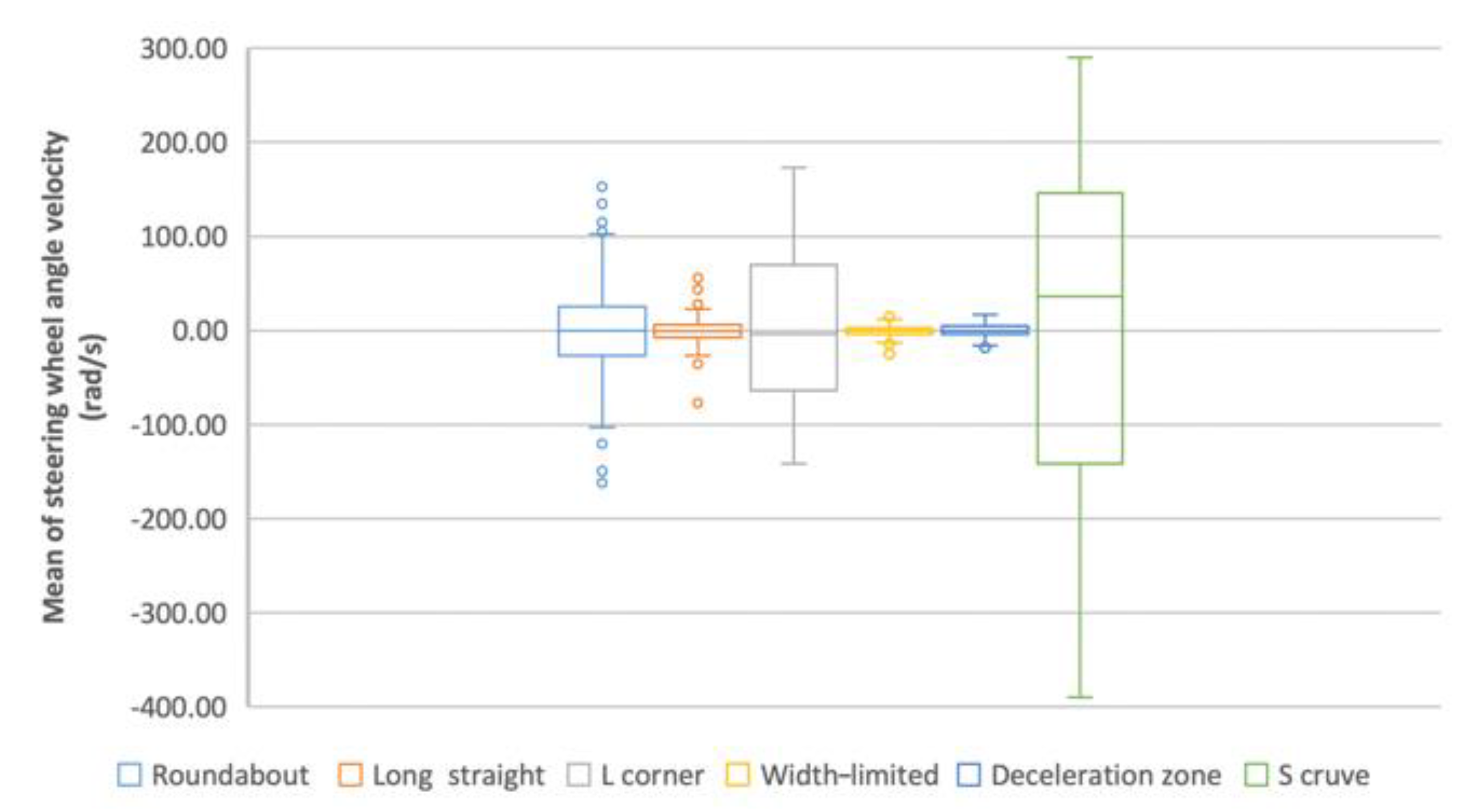
- From the box plot (Figure 14), the distribution of SWV values is analogous between long straight, width-limited and deceleration zone, while the distribution of others is varied.
- (b)
- From the radar chart (Figure 4), the distance among width-limited, deceleration zone and L-corner is small and close to the center of the circle, which is consistent with (a) and (c).
- (c)
- From the ANOVA (Table 12), no significant differences appear between any scenes.
- (d)
- Summary: The SWV in each scene shows little significance; thus, it cannot be used to represent the driving control characteristic in any driving scenes.
3.5.5. Mean of Steering Wheel Angle Velocity
- (a)
- From the box plot (Figure 15), the distribution of M-SWV values is analogous between width-limited and deceleration zone, while the distribution of others is varied.
- (b)
- From the radar chart (Figure 4), the distance among width-limited, deceleration zone and L-corner is small and close to the center of the circle.
- (c)
- From the ANOVA (Table 13), no significant differences appear between any scenes.
- (d)
- Summary: The results of (a), (b) and (c) cannot achieve mutual authentication; the M-SWV is thus not applicable.
3.5.6. Standard Deviation of Steering Wheel Angle Velocity
- (a)
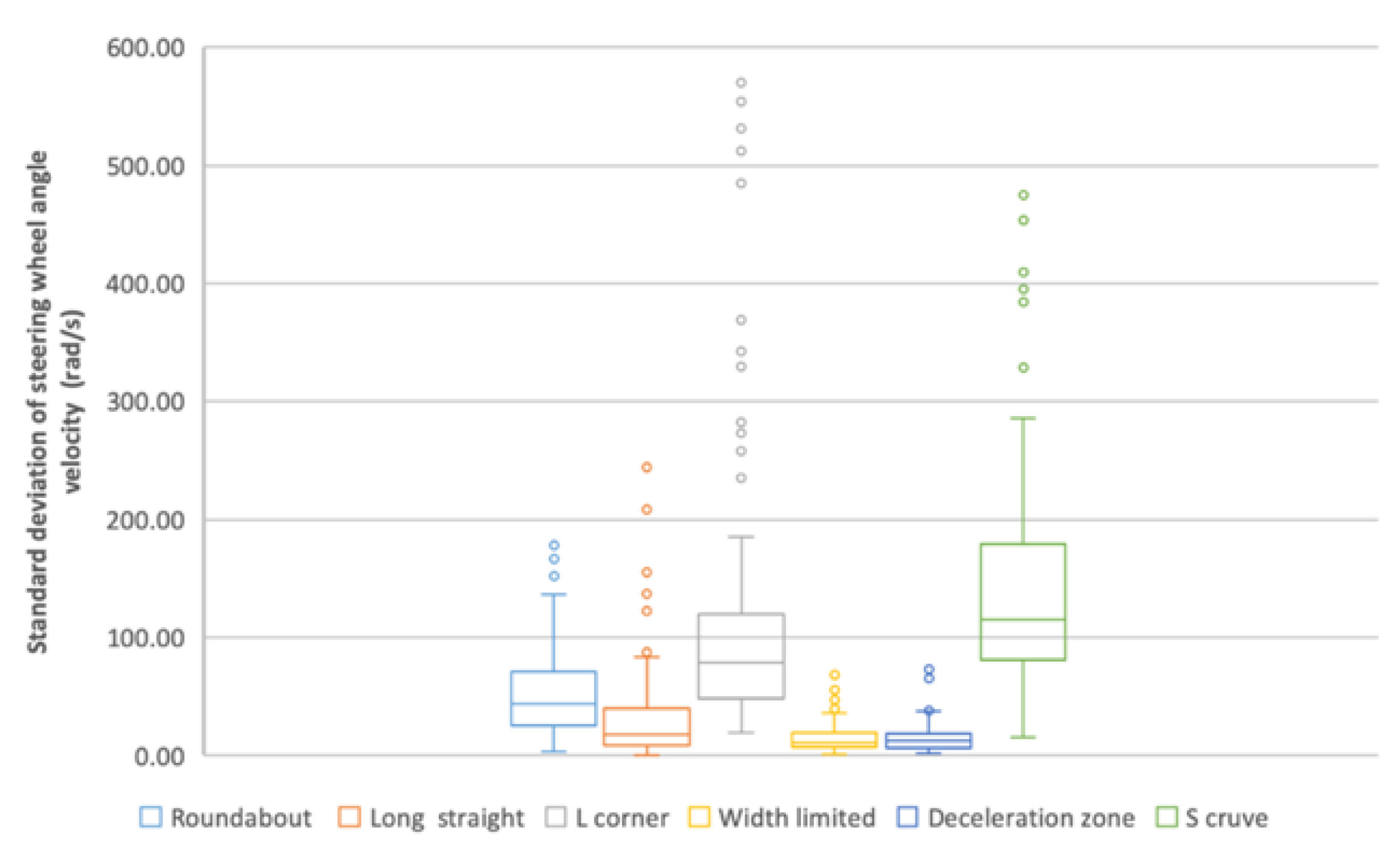
- From the box plot (Figure 16), the distribution of SD-SWV values is analogous among long straight, width-limited and deceleration zone, while the distribution of others is varied, which is consistent with (c).
- (b)
- From the radar chart (Figure 4), the distance between width-limited and deceleration zone is small and close to the center of the circle, which is consistent with (a).
- (c)
- From the ANOVA (Table 14), no significant differences appear between long straight and width-limited, or between long straight and deceleration zone.
- (d)
- Summary: The SD-SWV can be used to represent the driving control characteristic in driving scenes including roundabout, L-corner and S-curve.
3.5.7. Lateral Acceleration
- (a)
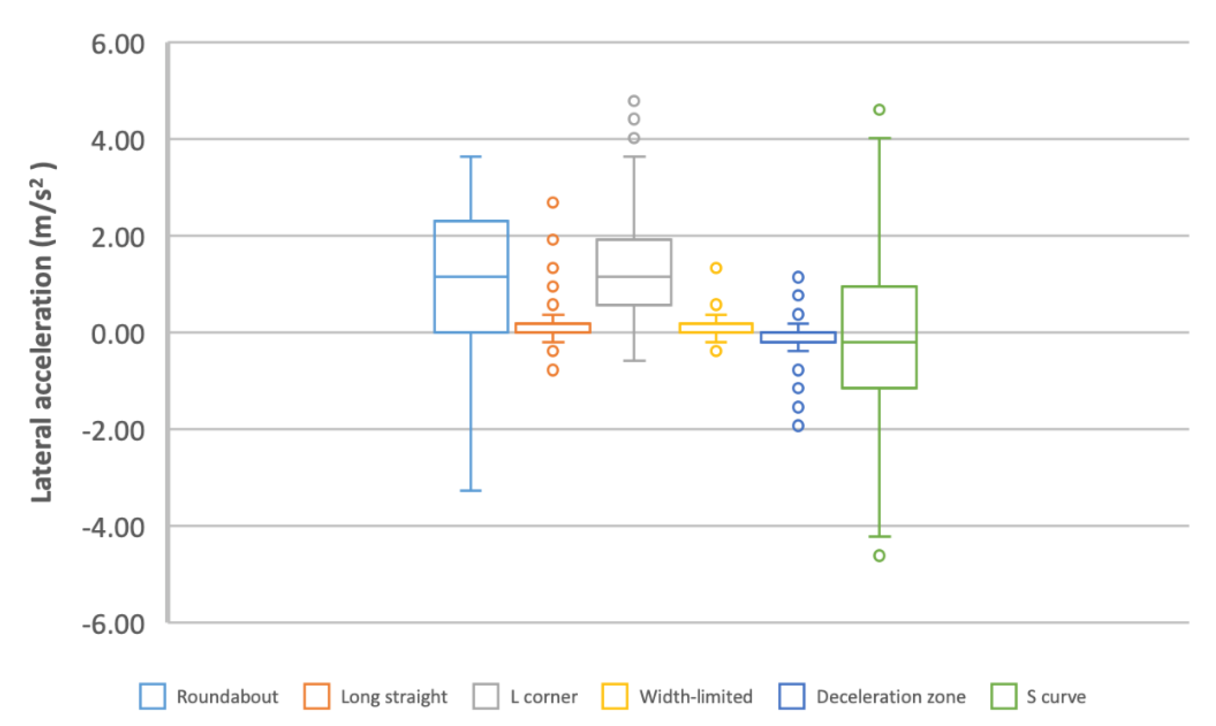
- From the box plot (Figure 17), the distribution of LAA values is analogous between long straight and width-limited, while the distribution of others is varied, which is consistent with (c).
- (b)
- From the radar chart (Figure 4), the distance between width-limited and deceleration zone is small and close to the center.
- (c)
- From the ANOVA (Table 15), no significant differences appear between long straight and width-limited, or between long straight and deceleration zone.
- (d)
- Summary: The LAA can be used to represent the driving control characteristic in driving scenes including roundabout, L-corner and S-curve.
3.5.8. Mean of Lateral Acceleration
- (a)
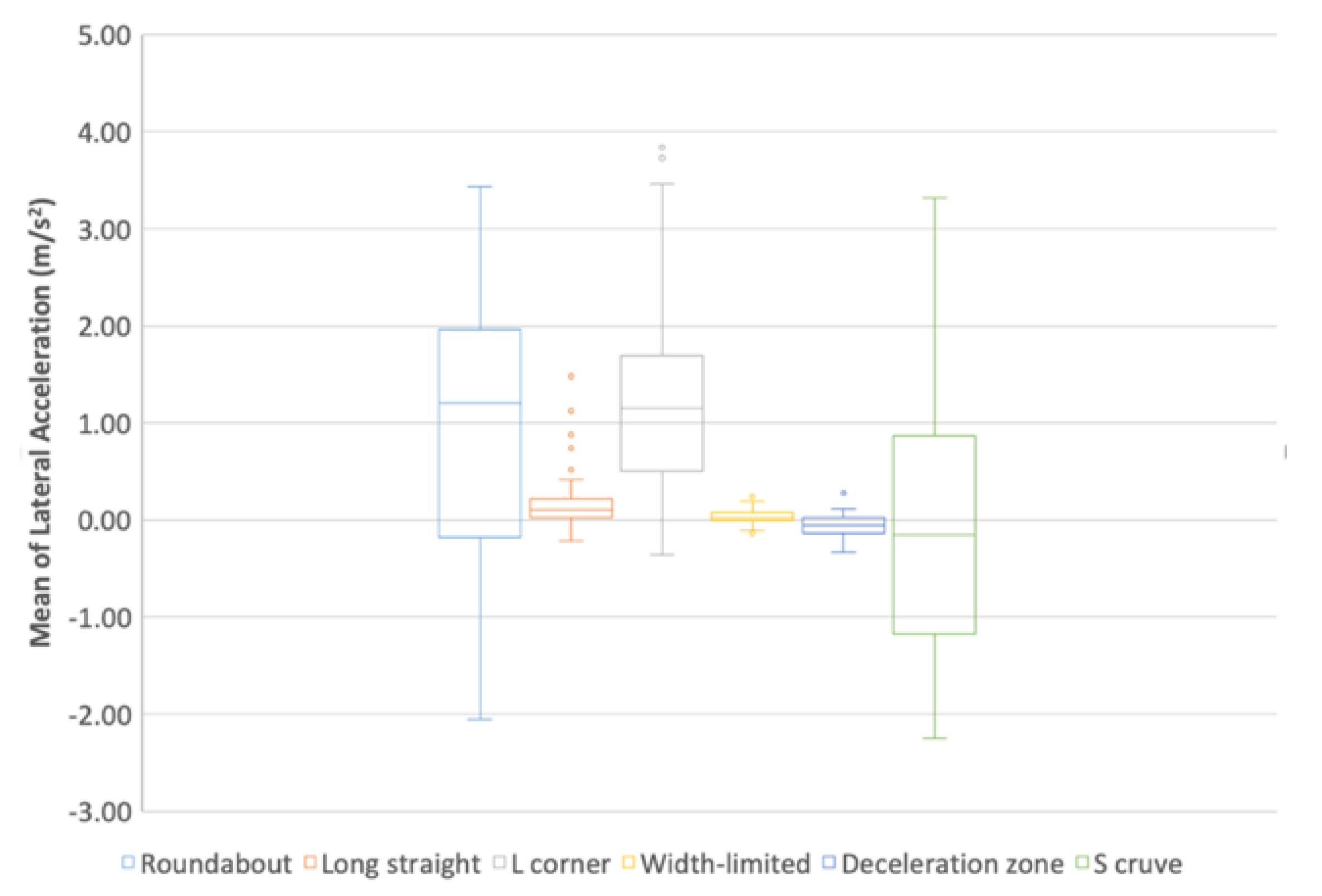
- From the box plot (Figure 18), the distribution of M-LAA values is analogous between long straight and width-limited, while the distribution of others is varied, which is consistent with (c).
- (b)
- From the radar chart (Figure 4), the distance of width-limited is close to the center, which is consistent with (a).
- (c)
- From the ANOVA (Table 16), no significant differences appear between long straight and width-limited, which is consistent with (b).
- (d)
- Summary: The M-LAA can be used to represent the driving control characteristic in driving scenes including roundabout, L-corner, deceleration zone and S-curve.
3.5.9. Standard Deviation of Lateral Acceleration
- (a)
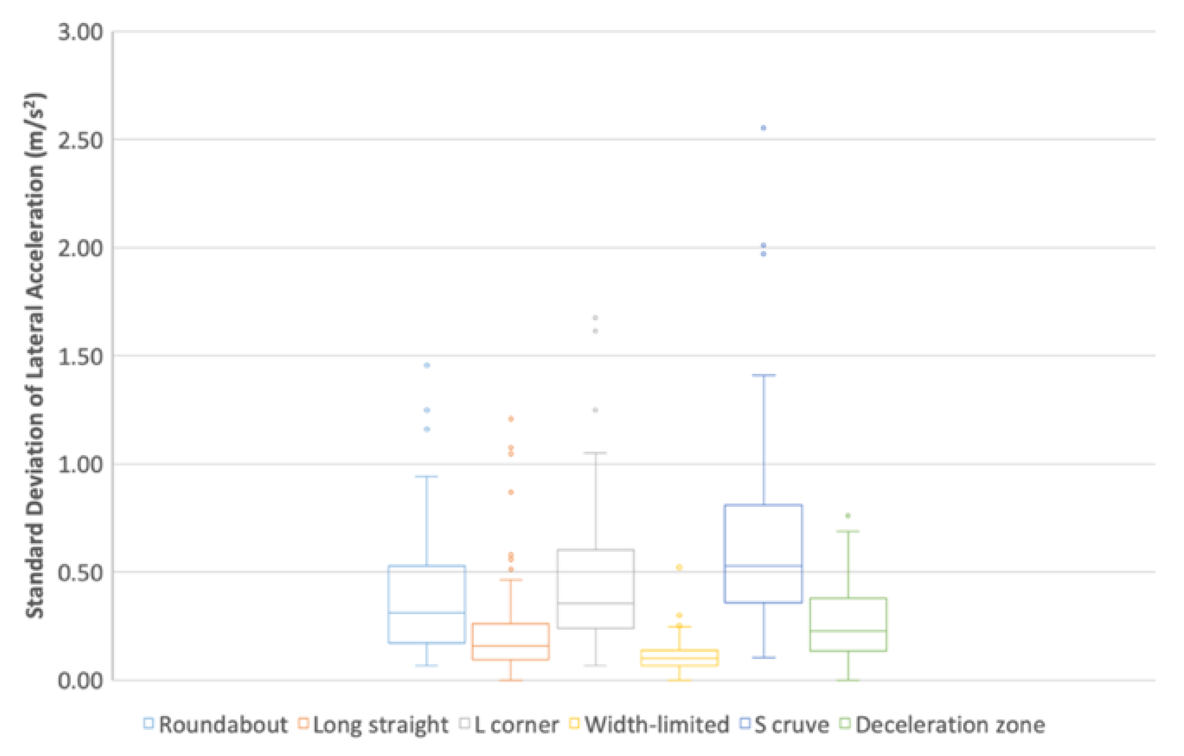
- From the box plot (Figure 19), the distributions of SD-LAA values are different, which is consistent with (c).
- (b)
- From the radar chart (Figure 4), the distances between each index and the long straight scene are different and far from the center, which is consistent with (a).
- (c)
- From the ANOVA (Table 17), significant differences appear between long straight and each index, which is consistent with (a) and (b).
- (d)
- Summary: The SD-LAA can be used to represent the driving control characteristic in all six driving scenes.
4. Results
- (a)
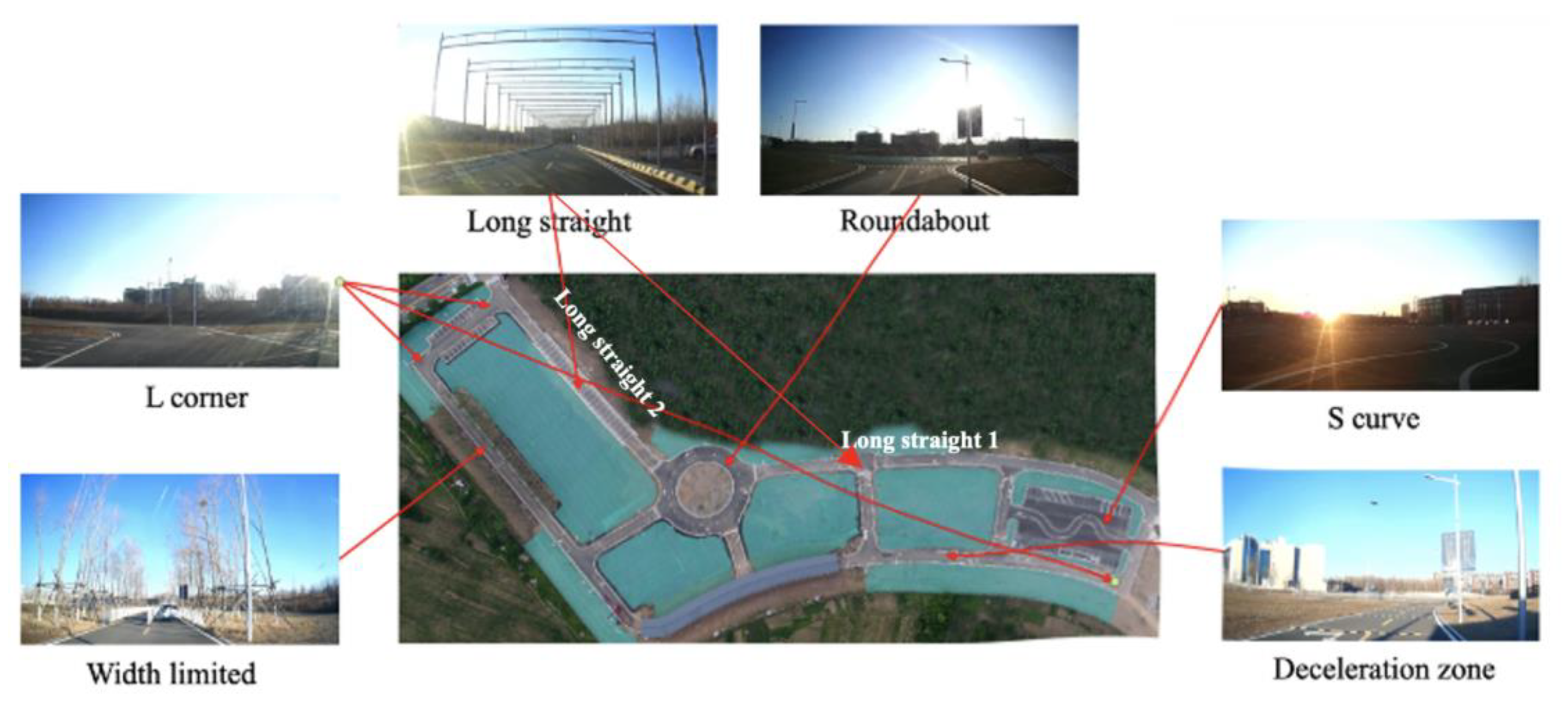
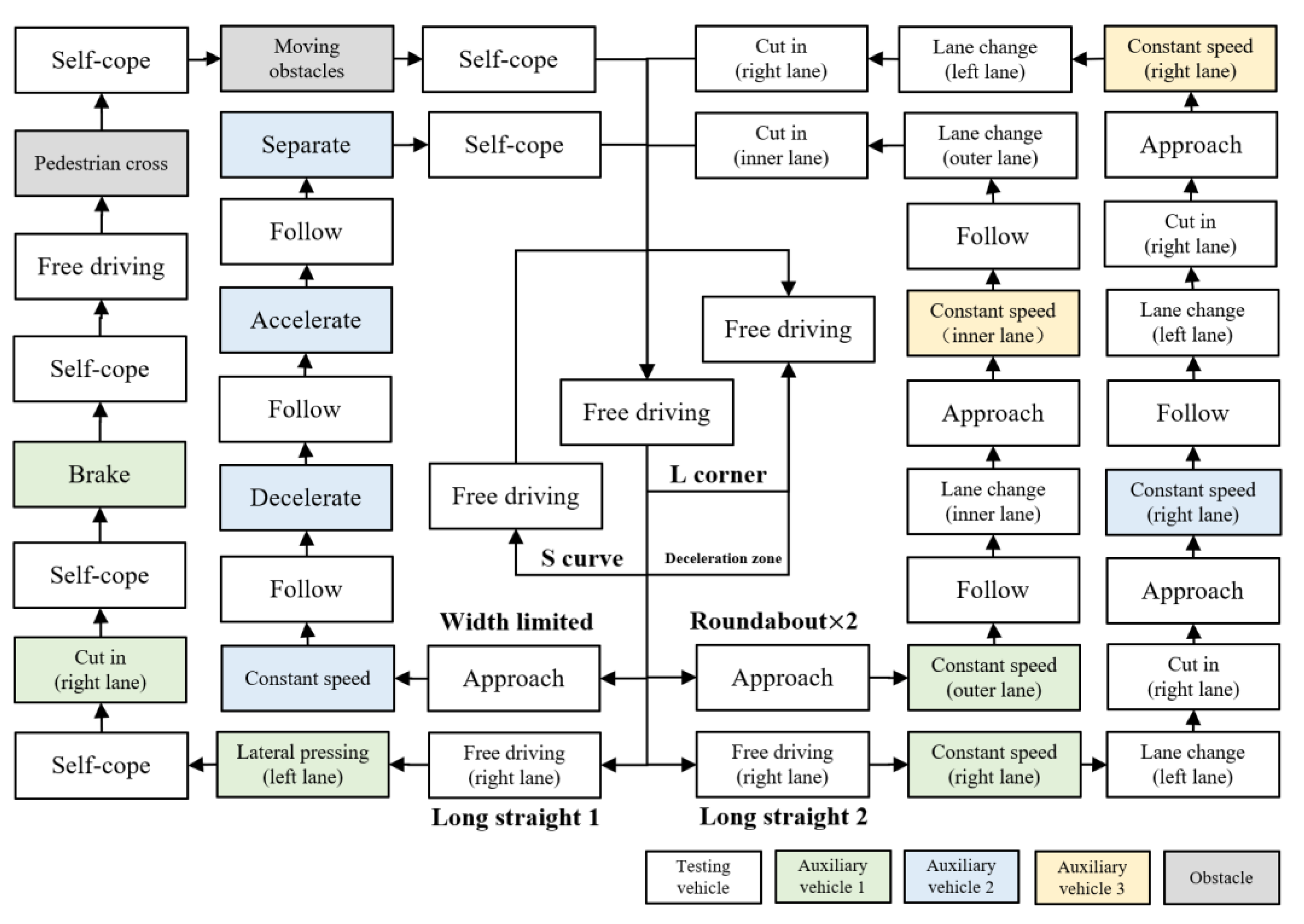
- The multi-vehicle interaction behavior in the long straight segment includes passive interference and active driving tasks. The specific driving performance of the road is to avoid the interference of other vehicles or moving obstacles, and to continuously change lanes to overtake them. The driver’s lateral and longitudinal vehicle control ability was mainly investigated. The quantitative indices included braking force, longitudinal velocity, lateral acceleration, yaw rate and their derivative variables. The weights of the lateral indices were greater than those of the longitudinal ones, which indicates that the driving task of this segment was more an investigation of lateral driving control ability.
- (b)
- This section mainly focused on lane change and cut-in behaviors in a long curve, and mainly investigated the driver’s ability to control the vehicle laterally and longitudinally. The quantitative indices included braking force, lateral acceleration, longitudinal speed, yaw rate, steering wheel angle and their derivative variables. Most of them were transverse indicators, but the weight of longitudinal indicators was large, which shows that these two kinds of indices are essential.
- (c)
- The width-limited segment mainly investigated variable speed car-following in a single lane so as to observe the longitudinal driving control characteristics of drivers. The quantitative indices included longitudinal velocity, lateral acceleration and their derivatives. SD-LAA reflects the change rate of lateral acceleration. Since there was almost no lateral velocity fluctuation in this scene, the SD-LAA was different from that in other scenarios, so that it is the characteristic index of this scene. These two kinds of indices can be mapped from the two-dimensional direction of the vehicle to the width-limited scene.
- (d)
- The indices in L-corner and S-curve included steering wheel angle, longitudinal velocity, braking force, yaw rate, lateral acceleration and their derivatives. According to the weight of each index, it can be found that although there was no interference from other vehicles, these two segments have high requirements for the driver’s lateral and longitudinal manipulation, and more indices are needed to reflect their characteristics.
- (e)
- The indexes in the deceleration zone segment included longitudinal velocity, braking force, lateral acceleration and their derivatives. It mainly investigated the vehicle driving control state of experienced drivers when passing through a continuous forced-deceleration zone. In addition, the meaning of the lateral acceleration derived index is similar to that of (c).
5. Summaries and Conclusions
5.1. Conclusions
- (1)
- The conclusion of this study is based on a real vehicle test. Although there may be some uncertain factors in the actual environment compared with the non-real driving experience of the simulator, our advantage is that we can extract completely real driver control characteristics, which are conducive to completely reflecting the characteristics of driver behavior changes.
- (2)
- Application innovation of method: By strictly comparing the data of drivers’ maneuvering performance and road types (data distribution analysis and relative difference calculation, etc.), this cross-analysis method can better determine which indicators in different scenarios have unique rules.
- (3)
- A better explanation of driver–roadway interaction can enhance road design to create a safer traffic system. Moreover, it can also provide basic support for human-like driving or for simulating the driving habits of experienced drivers. This study discusses the handling characteristic indicators of experienced drivers in different driving scenes. Subsequent studies can cite this method or its conclusions to train humanoid driving models so that the models can possess the characteristics of experienced drivers in these scenes.
5.2. Limitations and Prospects
Author Contributions
Funding
Institutional Review Board Statement
Informed Consent Statement
Data Availability Statement
Conflicts of Interest
References
- National Highway Traffic Safety Administration. Traffic Safety Facts 2011 Data: Rural/Urban Comparison; National Highway Traffic Safety Administration: Washington, DC, USA, 2013. [Google Scholar]
- Bobermin, M.P.; Silva, M.M.; Ferreira, S. Driving simulators to evaluate road geometric design effects on driver behaviour: A systematic review. Accid. Anal. Prev. 2020, 150, 105923. [Google Scholar] [CrossRef]
- Wåhlberg, A.A. Speed choice versus celeration behavior as traffic accident predictor. J. Saf. Res. 2006, 37, 43–51. [Google Scholar] [CrossRef] [PubMed]
- Simons-Morton, B.G.; Ouimet, M.C.; Zhang, Z.; Klauer, S.; Lee, S.E.; Wang, J.; Albert, P.S.; Dingus, T.A. Crash and Risky Driving Involvement Among Novice Adolescent Drivers and Their Parents. Am. J. Public Health 2011, 101, 2362–2367. [Google Scholar] [CrossRef]
- Simons-Morton, B.G.; Cheon, K.; Guo, F.; Albert, P. Trajectories of kinematic risky driving among novice teenagers. Accid. Anal. Prev. 2013, 51, 27–32. [Google Scholar] [CrossRef] [Green Version]
- Toledo, T.; Musicant, O.; Lotan, T. In-vehicle data recorders for monitoring and feedback on drivers’ behavior. Transp. Res. Part C Emerg. Technol. 2008, 16, 320–331. [Google Scholar] [CrossRef]
- Mikolajetz, A.; Henning, M.J.; Tenzer, A.; Zobel, R.; Krems, J.F.; Petzoldt, T. Curve negotiation: Identifying driver behavior around curves with the driver performance database. In Proceedings of the Fifth International Driving Symposium on Human Factors in Driver Assessment, Training and Vehicle Design, Big Sky, MT, USA, 22–25 June 2009. [Google Scholar]
- Alsaid, A.; Lee, J.D.; Price, M. Moving into the Loop: An Investigation of Drivers’ Steering Behavior in Highly Automated Vehicles. Hum. Factors J. Hum. Factors Ergon. Soc. 2019, 62, 671–683. [Google Scholar] [CrossRef] [PubMed]
- Sparrow, A.R.; Lajambe, C.M.; Van Dongen, H.P.A. Drowsiness measures for commercial motor vehicle operations. Accid. Anal. Prev. 2019, 126, 146–159. [Google Scholar] [CrossRef] [PubMed]
- Wu, K.-F.; Jovanis, P.P. Defining and screening crash surrogate events using naturalistic driving data. Accid. Anal. Prev. 2013, 61, 10–22. [Google Scholar] [CrossRef]
- Dong, Y.; Hu, Z.; Uchimura, K.; Murayama, N. Driver Inattention Monitoring System for Intelligent Vehicles: A Review. IEEE Trans. Intell. Transp. Syst. 2010, 12, 596–614. [Google Scholar] [CrossRef]
- Farahmand, B.; Boroujerdian, A.M. Effect of road geometry on driver fatigue in monotonous environments: A simulator study. Transp. Res. Part F Traffic Psychol. Behav. 2018, 58, 640–651. [Google Scholar] [CrossRef]
- Guo, B.; Jin, L.; Sun, D.; Shi, J.; Wang, F. Establishment of the characteristic evaluation index system of sec-ondary task driving and analyzing its importance. Transp. Res. F Traffic Psychol. Behav. 2019, 64, 308–317. [Google Scholar] [CrossRef]
- Kaur, R.; Sharma, S. Analysis of driver’s characteristics on a curved road in a lattice model. Phys. A Stat. Mech. Appl. 2017, 471, 59–67. [Google Scholar] [CrossRef]
- Gu, T.; Dolan, J.M. Toward human-like motion planning in urban environments. In Proceedings of the 2014 IEEE Intelligent Vehicles Symposium Proceedings, Dearborn, MI, USA, 8–11 June 2014; pp. 350–355. [Google Scholar]
- Kang, X.; Namgung, M.; Fujiwara, A.; Kim, W.; Wang, W. Analysis of Vehicle Maneuverability and Driving Characteristics on a Curved Road Condition. KSCE J. Civ. Eng. 2018, 23, 420–432. [Google Scholar] [CrossRef]
- Cerni, G.; Bassani, M. Naturalistic driving data collection to investigate into the effects of road geometrics on track behaviour. Transp. Res. Part C Emerg. Technol. 2017, 77, 1–15. [Google Scholar] [CrossRef]
- Wandtner, B.; Schömig, N.; Schmidt, G.J. Secondary task engagement and disengagement in the context of highly automated driving. Transp. Res. F: Traffic Psychol. Behav. 2018, 58, 253–263. [Google Scholar] [CrossRef]
- Papadimitriou, E.; Filtness, A.; Theofilatos, A.; Ziakopoulos, A.; Quigley, C.; Yannis, G. Review and ranking of crash risk factors related to the road infrastructure. Accid. Anal. Prev. 2019, 125, 85–97. [Google Scholar] [CrossRef] [Green Version]
- Zia, H.; Harris, D.; Smith, D. Infrastructure Risk Rating Manual for Australian Roads No. AP-R587A-19; ARRB: Vermont South, Australia, 2019. [Google Scholar]
- Chu, D.; Deng, Z.; He, Y.; Wu, C.; Sun, C.; Lu, Z. Curve speed model for driver assistance based on driving style classification. IET Intell. Transp. Syst. 2017, 11, 501–510. [Google Scholar] [CrossRef]
- Carsten, O.; Lai, F.; Barnard, Y.; Jamson, A.H.; Merat, N. Control Task Substitution in Semiautomated Driving: Does It Matter What Aspects Are Automated? Hum. Factors 2012, 54, 747–761. [Google Scholar] [CrossRef] [Green Version]
- Zhao, S.-F.; Guo, W.; Zhang, C.-W. Extraction Method of Driver’s Mental Component Based on Empirical Mode Decomposition and Approximate Entropy Statistic Characteristic in Vehicle Running State. J. Adv. Transp. 2017, 2017, 9509213. [Google Scholar] [CrossRef]
- Hou, M.; Lin, Z.; Chen, J.; Zhai, Y.; Jin, Q.; Zhong, F. Optimization on the Buried Depth of Subsurface Drainage under Greenhouse Condition Based on Entropy Evaluation Method. Entropy 2018, 20, 859. [Google Scholar] [CrossRef] [Green Version]
- He, D.; Xu, J.; Chen, X. Information-Theoretic-Entropy Based Weight Aggregation Method in Multiple-Attribute Group Decision-Making. Entropy 2016, 18, 171. [Google Scholar] [CrossRef] [Green Version]
- Ji, Y.; Huang, G.H.; Sun, W. Risk assessment of hydropower stations through an integrated fuzzy entropy-weight multiple criteria decision making method: A case study of the Xiangxi River. Expert Syst. Appl. 2015, 42, 5380–5389. [Google Scholar] [CrossRef]
- Jin, L.; Guo, B.; Jiang, Y.; Wang, F.; Xie, X.; Gao, M. Study on the Impact Degrees of Several Driving Behaviors When Driving While Performing Secondary Tasks. IEEE Access 2018, 6, 65772–65782. [Google Scholar] [CrossRef]
- Shih, H.-S.; Shyur, H.-J.; Lee, E.S. An extension of TOPSIS for group decision making. Math. Comput. Model. 2007, 45, 801–813. [Google Scholar] [CrossRef]
- Calvi, A. A Study on Driving Performance Along Horizontal Curves of Rural Roads. J. Transp. Saf. Secur. 2014, 7, 243–267. [Google Scholar] [CrossRef]
- Bobermin, M.P.; Silva, M.M.; Ferreira, S.; Guedes, J.C.C.; Baptista, J.S. Driving simulator for evaluating the effects of road geometric design on driver behavior: Protocol of a systematic review. Int. J. Occup. Environ. Saf. 2019, 3, 46–51. [Google Scholar] [CrossRef]
- Choudhari, T.; Maji, A. Assessment of Driver Performance Based on Driver Demography and Road Geometry (No. 18–06523). In Proceedings of the Transportation Research Board 97th Annual Meeting, Washington, DC, USA, 7–11 January 2018. [Google Scholar]
- De Ona, J.; López, G.; Mujalli, R.; Calvo, F.J. Analysis of traffic accidents on rural highways using Latent Class Clustering and Bayesian Networks. Accid. Anal. Prev. 2013, 51, 1–10. [Google Scholar] [CrossRef] [PubMed] [Green Version]
- Bella, F. Driver perception hypothesis: Driving simulator study. Transp. Res. F Traffic Psychol. Behav. 2014, 24, 183–196. [Google Scholar] [CrossRef]


| Vehicle Running State | Hypothetical Characteristic Parameters | Abbreviation |
|---|---|---|
| Longitudinal direction | Longitudinal velocity | LOV |
| Mean of longitudinal velocity | M-LOV | |
| Standard deviation of longitudinal velocity | SD-LOV | |
| Longitudinal acceleration | LOA | |
| Mean of longitudinal acceleration | M-LOA | |
| Standard deviation of longitudinal acceleration | SD-LOA | |
| Braking force | BF | |
| Mean of braking force | M-BF | |
| Standard deviation of braking force | SD-BF | |
| Lateral direction | Yaw rate | YR |
| Mean of yaw rate | M-YR | |
| Standard deviation of yaw rate | SD-YR | |
| Steering wheel angle velocity | SWV | |
| Mean of steering wheel angle velocity | M-SWV | |
| Standard deviation of steering wheel angle velocity | SD-SWV | |
| Lateral acceleration | LAA | |
| Mean of lateral acceleration | M-LAA | |
| Standard deviation of lateral acceleration | SD-LAA |
| Evaluation Index | Roundabout | Long Straight | L-Corner | Width-Limited | Deceleration Zone | S-Curve |
|---|---|---|---|---|---|---|
| LOV | 0.206 | 0.140 | 0.220 | 0.161 | 0.153 | 0.120 |
| M-LOV | 0.255 | 0.146 | 0.231 | 0.113 | 0.085 | 0.169 |
| SD-LOV | 0.206 | 0.205 | 0.129 | 0.180 | 0.136 | 0.144 |
| LOA | 0.347 | 0.073 | 0.032 | 0.017 | 0.039 | 0.493 |
| M-LOA | 0.339 | 0.272 | 0.081 | 0.079 | 0.094 | 0.134 |
| SD-LOA | 0.174 | 0.251 | 0.146 | 0.198 | 0.117 | 0.115 |
| BF | 0.181 | 0.204 | 0.064 | 0.291 | 0.182 | 0.078 |
| M-BF | 0.244 | 0.145 | 0.189 | 0.096 | 0.194 | 0.133 |
| SD-BF | 0.226 | 0.126 | 0.176 | 0.141 | 0.202 | 0.129 |
| YR | 0.154 | 0.171 | 0.182 | 0.168 | 0.166 | 0.159 |
| M-YR | 0.142 | 0.159 | 0.154 | 0.244 | 0.151 | 0.150 |
| SD-YR | 0.197 | 0.222 | 0.134 | 0.213 | 0.103 | 0.131 |
| SWV | 0.260 | 0.040 | 0.080 | 0.170 | 0.150 | 0.290 |
| M-SWV | 0.130 | 0.050 | 0.36 | 0.08 | 0.150 | 0.230 |
| SD-SWV | 0.110 | 0.246 | 0.231 | 0.140 | 0.150 | 0.123 |
| LAA | 0.163 | 0.167 | 0.325 | 0.156 | 0.049 | 0.139 |
| M-LAA | 0.201 | 0.255 | 0.177 | 0.158 | 0.110 | 0.100 |
| SD-LAA | 0.224 | 0.195 | 0.175 | 0.127 | 0.106 | 0.173 |
| Driving Scenes | Mean Difference | Sig. | |
|---|---|---|---|
| Long straight | Roundabout | 4.904 * | 0.000 |
| L-corner | 7.276 * | 0.000 | |
| Width-limited | −2.838 * | 0.000 | |
| Deceleration | 6.108 * | 0.000 | |
| S-curve | 11.885 * | 0.000 | |
| Driving Scenes | Mean Difference | Sig. | |
|---|---|---|---|
| Long straight | Roundabout | 4.904 * | 0.000 |
| L-corner | 7.273 * | 0.000 | |
| Width-limited | −2.850 * | 0.006 | |
| Deceleration | 6.206 * | 0.000 | |
| S-curve | 11.885 * | 0.000 | |
| Driving Scenes | Mean Difference | Sig. | |
|---|---|---|---|
| Long straight | Roundabout | 1.629 * | 0.000 |
| L-corner | 0.779 * | 0.001 | |
| Width-limited | 1.027 * | 0.000 | |
| Deceleration | 0.985 * | 0.002 | |
| S-curve | 1.635 * | 0.000 | |
| Driving Scenes | Mean Difference | Sig. | |
|---|---|---|---|
| Long straight | Roundabout | 4.098 * | 0.000 |
| L-corner | 3.583 * | 0.000 | |
| Width-limited | 4.301 * | 0.000 | |
| Deceleration | 3.019 * | 0.000 | |
| S-curve | 4.222 * | 0.000 | |
| Driving Scenes | Mean Difference | Sig. | |
|---|---|---|---|
| Long straight | Roundabout | 4.119 * | 0.000 |
| L-corner | 3.601 * | 0.000 | |
| Width-limited | 4.344 * | 0.000 | |
| Deceleration | 3.045 * | 0.000 | |
| S-curve | 4.242 * | 0.000 | |
| Driving Scenes | Mean Difference | Sig. | |
|---|---|---|---|
| Long straight | Roundabout | 1.820 * | 0.000 |
| L-corner | 1.275 * | 0.000 | |
| Width-limited | 2.004 * | 0.000 | |
| Deceleration | 0.568 * | 0.000 | |
| S-curve | 1.896 * | 0.000 | |
| Driving Scenes | Mean Difference | Sig. | |
|---|---|---|---|
| Long straight | Roundabout | −8.246 * | 0.000 |
| L-corner | −12.390 * | 0.000 | |
| Width-limited | 0.677 | 0.290 | |
| Deceleration | 0.583 | 0.106 | |
| S-curve | 1.535 * | 0.019 | |
| Driving Scenes | Mean Difference | Sig. | |
|---|---|---|---|
| Long straight | Roundabout | −8.375 * | 0.000 |
| L-corner | −12.418 * | 0.000 | |
| Width-limited | 0.640 | 0.529 | |
| Deceleration | 1.941 | 0.091 | |
| S-curve | 1.487 | 0.150 | |
| Driving Scenes | Mean Difference | Sig. | |
|---|---|---|---|
| Long straight | Roundabout | −1.712 * | 0.000 |
| L-corner | −3.602 * | 0.000 | |
| Width-limited | 0.643 * | 0.009 | |
| Deceleration | 0.587 * | 0.036 | |
| S-curve | −6.847 * | 0.000 | |
| Driving Scenes | Mean Difference | Sig. | |
|---|---|---|---|
| Long straight | Roundabout | 1.392 | 0.811 |
| L-corner | 1.313 | 0.829 | |
| Width-limited | 1.628 | 0.813 | |
| Deceleration | 1.355 | 0.861 | |
| S-curve | 3.405 | 0.621 | |
| Driving Scenes | Mean Difference | Sig. | |
|---|---|---|---|
| Long straight | Roundabout | 1.133 | 0.853 |
| L-corner | 3.178 | 0.619 | |
| Width-limited | 0.990 | 0.891 | |
| Deceleration | 0.795 | 0.923 | |
| S-curve | 2.179 | 0.763 | |
| Driving Scenes | Mean Difference | Sig. | |
|---|---|---|---|
| Long straight | Roundabout | −15.239 * | 0.006 |
| L-corner | −78.603 * | 0.000 | |
| Width-limited | 13.879 | 0.053 | |
| Deceleration | 13.534 | 0.070 | |
| S-curve | −107.334 * | 0.000 | |
| Driving Scenes | Mean Difference | Sig. | |
|---|---|---|---|
| Long straight | Roundabout | −0.798 * | 0.000 |
| L-corner | −1.025 * | 0.000 | |
| Width-limited | 0.111 | 0.052 | |
| Deceleration | 0.234 * | 0.000 | |
| S-curve | 0.248 * | 0.000 | |
| Driving Scenes | Mean Difference | Sig. | |
|---|---|---|---|
| Long straight | Roundabout | −0.791 * | 0.000 |
| L-corner | −1.016 * | 0.000 | |
| Width-limited | 0.126 | 0.155 | |
| Deceleration | 0.256 * | 0.010 | |
| S-curve | 0.262 * | 0.003 | |
| Driving Scenes | Mean Difference | Sig. | |
|---|---|---|---|
| Long straight | Roundabout | −0.138 * | 0.000 |
| L-corner | −0.213 * | 0.000 | |
| Width-limited | 0.115 * | 0.000 | |
| Deceleration | −0.057 * | 0.050 | |
| S-curve | −0.404 * | 0.000 | |
Publisher’s Note: MDPI stays neutral with regard to jurisdictional claims in published maps and institutional affiliations. |
© 2022 by the authors. Licensee MDPI, Basel, Switzerland. This article is an open access article distributed under the terms and conditions of the Creative Commons Attribution (CC BY) license (https://creativecommons.org/licenses/by/4.0/).
Share and Cite
Guo, B.; Hua, Q.; Jin, L.; Xie, X.; Huo, Z.; Wang, H. Analysis of Driving Control Characteristics in Typical Road Types. Sustainability 2022, 14, 782. https://doi.org/10.3390/su14020782
Guo B, Hua Q, Jin L, Xie X, Huo Z, Wang H. Analysis of Driving Control Characteristics in Typical Road Types. Sustainability. 2022; 14(2):782. https://doi.org/10.3390/su14020782
Chicago/Turabian StyleGuo, Baicang, Qiang Hua, Lisheng Jin, Xianyi Xie, Zhen Huo, and Huanhuan Wang. 2022. "Analysis of Driving Control Characteristics in Typical Road Types" Sustainability 14, no. 2: 782. https://doi.org/10.3390/su14020782
APA StyleGuo, B., Hua, Q., Jin, L., Xie, X., Huo, Z., & Wang, H. (2022). Analysis of Driving Control Characteristics in Typical Road Types. Sustainability, 14(2), 782. https://doi.org/10.3390/su14020782


