Article

Simulation and Spatio-Temporal Variation Characteristics of LULC in the Context of Urbanization Construction and Ecological Restoration in the Yellow River Basin

1
School of Soil and Water Conservation, Beijing Forestry University, Beijing 100083, China
2
Key Laboratory of State Forestry Administration on Soil and Water Conservation and Desertification Combating, Beijing Forestry University, Beijing 100083, China
3
Jixian Research Station for Forest Ecosystem, CFERN/CNERN, Beijing Forestry University, Beijing 100083, China
*
Author to whom correspondence should be addressed.
Sustainability 2022, 14(2), 789; https://doi.org/10.3390/su14020789
Submission received: 5 November 2021 / Revised: 26 December 2021 / Accepted: 7 January 2022 / Published: 11 January 2022

Abstract

:
The Yellow River Basin (YRB), located in the northern region of China, has a fragile ecological environment. With the construction of urbanization and ecological restoration projects, the YRB LULC has undergone significant change. In this study, we used the coupled Markov-FLUS model by combining natural and social driver factors to predict and simulate the LULC of the YRB in 2030, and then the LULC transfer matrix was used to analyze the characteristics of LULC change in the YRB from 1990 to 2030. The results of the study are as follows. (1) For the simulated result of LULC compared with the same period observed result, the Kappa coefficient is 0.92, indicating the coupled Markov-FLUS model has good applicability in the YRB. (2) The LULC in the YRB shows significant spatial autocorrelation. The cropland is mainly distributed in the eastern region, which is dominated by plain; woodland is mainly distributed in the central region; grassland is mainly distributed in the northern, central, and western region; waterbody is mainly distributed in the western region; built-up land is mainly distributed in the northern, south-central, and eastern region; unused land is mainly distributed in the central, northern, and western region. (3) From 1990 to 2000, the area of cropland transferred in significantly and the area of grassland transferred out significantly; from 2000 to 2015, the area of construction land transferred in significantly and the area of cultivated land transferred out significantly; from 2015 to 2030, the amount of cropland transferred out will be large, and the conversion of each other LULC type will be not significant compared with the previous periods, and the conversion structure of LULC will tend to be stable. This study is a crucial reference value for the high-quality development of the Yellow River Basin.

1. Introduction

Land use/land cover (LULC) variation not only changes the original surface characteristics of a region [1,2] but also has important impact on the local physical and social geography environment [3,4], which has now become a hot research topic in international earth system science [5]. LULC change is a vital element of different natural and social environmental change such as the carbon cycle [6], hydrological characteristics [7], urban expansion [8,9], etc. Therefore, it is crucial for policy makers and researchers to rapidly and accurately predict and simulate the future LULC of a region and analyze its LULC spatio-temporal variation characteristics for land resource management, which is also considered as an important way to achieve regional sustainable development [10].
The emergence of new technologies such as Remote Sensing (RS), Geographic Information Systems (GIS), and Global Navigation Satellite System (GNSS) has made it possible for policy makers and researchers to explore LULC change efficiently, accurately, and systematically [11,12,13,14]. Based on RS, GIS and GNSS (3S) information technology, many scholars have conducted in-depth research on LULC in different regions from multiple dimensions or perspectives, such as spatio-temporal analysis, driving mechanism, prediction, and simulation, etc., and have achieved fruitful results [1,15,16,17,18,19,20]. However, the latest research points out that the basin as a geographical unit linking the upper, middle, and lower reaches of rivers, its information, function, and energy of its internal ecosystem are relatively independent, so it is more beneficial to predict and simulate its future LULC and analyze its spatio-temporal change characteristics to understand the regional ecological environment change and promote the construction of “mountain, water, woodland, field, lake and grass” in an integrated manner [21]. Nonetheless, few studies have predicted and simulated LULC from a complete basin-scale and analyzed its spatio-temporal change characteristics. Therefore, at this stage, there is a crucial need to predict and simulate LULC at the basin scale and analyze its LULC spatio-temporal variation characteristics.
The Yellow River Basin (YRB) is located in an arid, semi-arid and semi-humid region of China with a fragile ecological environment [22]. Since 1978, the Communist Party of China Central Committee and the State Council have implemented the “Reform and Opening-up” policy, which has greatly liberated and developed local productivity and accelerated urban development [23,24]. However, the inappropriate production and lifestyle of people has led to serious damage to the natural vegetation in the region and increased eco-environmental problem, such as desertification [23,25,26]. The Chinese government attaches great importance to the construction of the ecological environment in the YRB. Since 2000, to restore surface vegetation, improve vegetation cover and solve a series of ecological and environmental degradation problems, the Chinese government has implemented a series of large-scale ecological restoration projects in the region, such as the “the Three-North Shelter Forest Program” and the “Grain for Green” program [27,28,29]. Rapid urban development and implementation of ecological restoration projects have led to significant change of the LULC in the YRB [30]. Besides, in October 2021, the Communist Party of China Central Committee and the State Council promulgated an outline document on the ecological protection and high-quality development of the YRB [31]. The outline document points out that by 2030, the YRB ecological co-management, environmental protection, urban and rural areas to coordinate the pattern of joint development will gradually take shape, the quality of the ecological environment to be significantly improved [31]. Therefore, predicting and simulating the future LULC of the YRB and analyzing its LULC spatio-temporal variation characteristics is a useful attempt to provide a reasonable basis for ecological restoration and urbanization construction in the region.
Because the future LULC is an important basis for analyzing the spatio-temporal variation characteristics of the basin LULC, selecting a reliable method to predict and simulate the future LULC of the basin becomes critical for researchers. According to the principle of LULC predictive simulation, LULC predictive simulation can be divided into two modules: LULC demand prediction and LULC spatial simulation [10]. Logistic regression [32], system dynamics [33], multi-objective programming [34], Markov model [35] and Ant Colony Optimization models [36] are commonly used to predict LULC demand, i.e., to quantify LULC types demand in the future. The Markov model has become the preferred method for many scholars to predict LULC demand because of its ability to quantify future LULC types demand easily and accurately with less data. Currently, for LULC spatial simulation, Cellular Automata (CA)model [36], the Conversion of Land Use and its Effect at Small regional extent (CLUE-S) model [37] and the Future Land Use Simulation (FLUS) model [38] are often used to simulate the future LULC spatial distribution. Among them, the FLUS model is a simulation model of the future LULC that takes into account both the natural environment and the impact of human activities [38]. The FLUS model has been widely used for multi-category LULC simulations at various spatial scales because of its strong spatio-temporal dynamic simulation capability and efficient LULC simulation performance. For example, Li et al. simulated the global multi-category LULC spatial distribution from 2010 to 2100 [39]. Chen et al. simulated the 2040 LULC of the Hokkaido Japan in the context of different cropland policy [40]; Feng et al. simulated the 2034 LULC of the Qinghai lake basin [21]. Although the Markov model and FLUS model has been relatively mature and widely used for LULC demand prediction and LULC spatial simulation at multiple spatial scales, few scholars have used the Markov model and FLUS model to predict and simulate future LULC of the YRB to know its spatio-temporal variation characteristics.
Thus, in this study, we took the YRB as the study area and used the coupled Markov-FLUS model to predict and simulate the future LULC in the YRB (2030) in the context of ecological restoration and urban development, to provide the future LULC data of the YRB. Besides, different scenarios of the future LULC in the YRB are compared. Based on the past (1990–2015) and future (2030) LULC data, a transfer matrix was selected to explore the spatio-temporal variation characteristics of LULC in the YRB in different periods. This study can help policy makers and researchers visualize the characteristics of LULC changes in the YRB under the background of ecological restoration and urban development. This is an important guideline for rational planning of land in the YRB and timely adjustment of ecological restoration and urban development policies, which will contribute to the high-quality development of the Yellow River Basin.

2. Materials and Methods
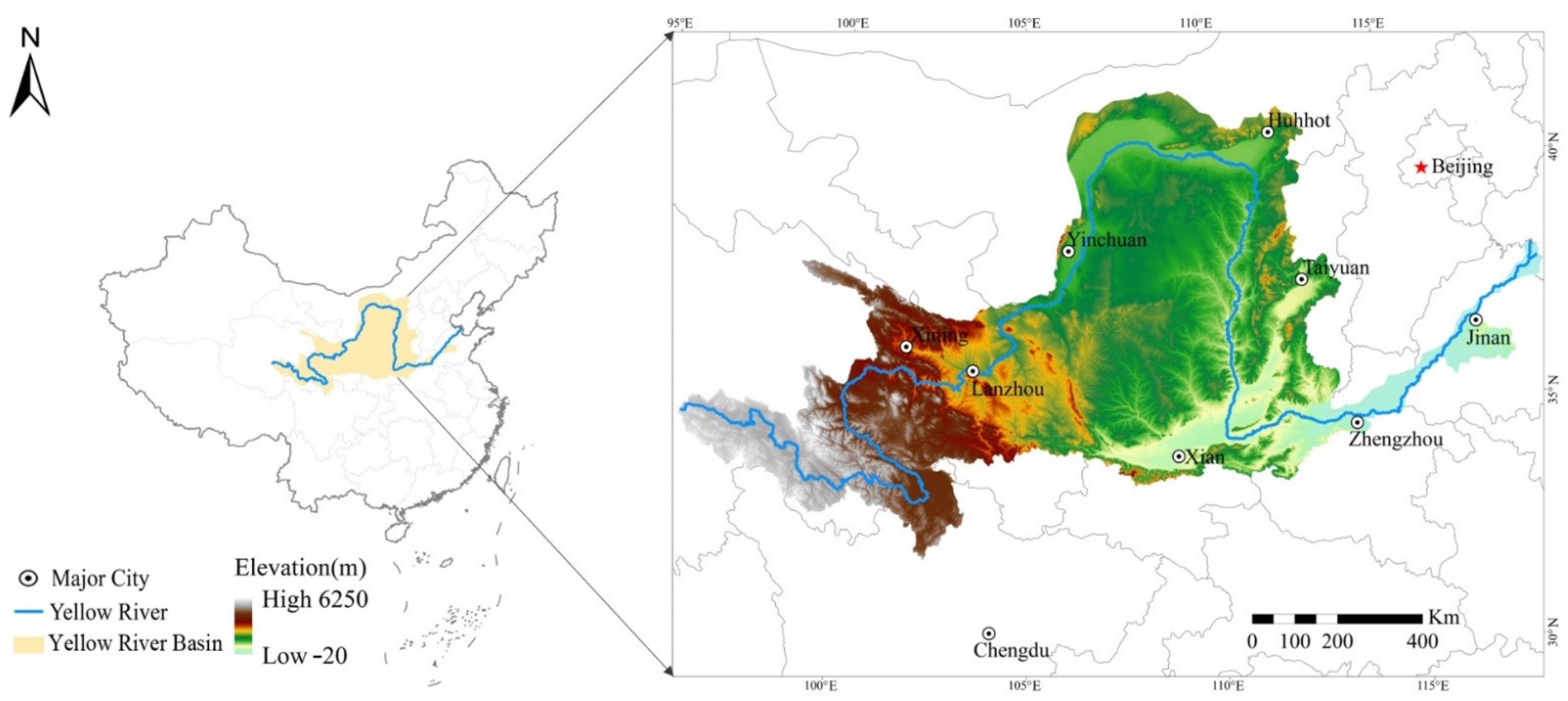
2.1. Study Area

The Yellow River originates from the Tibetan Plateau, flows from west to east through the Inner Mongolia Plateau, the Loess Plateau and the Yellow and Huaihai Plain, and finally injects into the Pacific Ocean, with a total length of about 5464 km. It is the fifth longest river in the world and the second longest in China and has had a profound impact on China’s natural environment and socio-economic development. The Yellow River Basin (96°−119° E, 32°−42° N) is connected to Kunlun Mountain in the west, Yinshan Mountain in the north, Qinling Mountain in the south, and Bohai Sea in the east, spanning the west, middle and east China [31], with a total area of about 7.95 × 10⁵ km2 [22], and is an important ecological security barrier in China (Figure 1). The topography of the area is high in the west and low in the east [41], with large undulations and complex landform types. The lowest elevation is −20 m, and the highest elevation is 6250 m in the YRB. The spatial distribution of precipitation is uneven throughout the region, with more in the east and less in the west, and most areas are located west of the 400 mm precipitation line, resulting in a shortage of water resources [42]; the annual average temperature is 2.68 °C [43], showing significant regional differences in temperature, with high temperatures in the east and low temperatures in the west, and large inter-annual variations. The YRB is also an important region for China’s population activities and economic development. Shanxi, Henan and Shandong provinces in the YRB are China’s major energy, food and industrial provinces, respectively, and have a pivotal strategic position in the construction of Chinese socialist modernization [31].

2.2. Data Source and Processing

The spatial dataset used to predict and simulate LULC in the YRB includes historical LULC data, topography (elevation and slope), meteorology (temperature and precipitation), soil (organic carbon, bulk density, and percentage of silt), and socio-human (population density, per capita GDP, distance to motor, distance to road and distance to railway) driving factor data. In particular, because large-scale artificial vegetation reconstruction projects are underway in the study area, vegetation has also become an important driving factor of LULC changes, so NDVI data were innovatively drawn into the driving factor data in this research.
Because LULC is the main object of this study, we first consider its spatio-temporal resolution and accessibility. The Resource and Environment Science and Data Center of the Institute of Geography and Resources, Chinese Academy of Sciences (http://www.resdc.cn/ (accessed on 25 August 2021)) provides free access to LULC data for the whole of China for 1990, 1995, 2000, 2005, 2010, 2015, 2018 and 2020. The dataset was generated by manual visual interpretation using Landsat TM/ETM/OLI remote sensing images of various phases as the main data source with a spatial resolution of 30 m. The LULC types were classified into six categories: cropland, woodland, grassland, waterbody, built-up land, and unused land (details are listed in Table 1). However, some driving factor datasets, such as precipitation, temperature, population density, and per capita GDP, are only provided up to 2015 on this website. Considering the availability of LULC and driving factor datasets, we selected LULC data for 1990, 2000 and 2015, where 2000 and 2015 data were used as model year data for predicting the 2030 YRB LULC. The Euclidean distance algorithm was used to convert the acquired vector data of motor, road, and railway in the study area into raster data of distance to motor, distance to road and distance to railway. To facilitate the calculation, all spatial data were reprojected as Albers equal-area conic projection (WGS_1984_Albers) with a spatial resolution resampling of 1 km, as shown in Figure 2. Details of LULC and driving factor data are listed in Table 2.

2.3. Methodology

In this study, we used Markov model to predict the each LULC type demand in the YRB based on the study area LULC data for 2000 and 2015. Then the FLUS model was used to simulate the LULC spatial distribution of the future scenario in the YRB, accounting to the calculated LULC types of demand by Markov model. Based on the LULC data from 1990 to 2030, spatio-temporal variation characteristics of LULC in the YRB were analyzed using the transfer matrix with 2000 and 2015 as time points to identify the characteristics of LULC changes in the YRB in different periods. The future scenario is that assuming the development of the study area will proceed without natural disasters or sudden fluctuations and changes in the economy and public policy in the near future. Therefore, the future scenario in this study means that the trend of LULC changes from 2000–2015 will remain unchanged until 2030. The methodological framework of this study is shown in Figure 3.

2.4. Methods

2.4.1. Coupled Markov-FLUS Model

(1) Markov model. A stochastic process is said to have Markovness (no posteriority) if, in a finite time sequence t1 < t2 < t3 < … < tn, the state an at any moment tn is only related to the state an−1 at the previous moment tn−1 [37,40]. Processes with Markov nature are called Markov processes. In the study of LULC change, the LULC change process can be regarded as a Markov process, and the LULC type at a certain moment corresponds to the possible states in the Markov process, which is only related to its LULC type at the previous moment, and the number or proportion of the area of interconversion between LULC types is the state transfer probability.
(2) FLUS model. The FLUS model is a LULC simulation model developed based on CA model but with several improvements over traditional CA, such as that the roulette wheel selection algorithm is introduced in the simulation process [38]. The model mechanism is as follows. First, in combination with the driving factors, an artificial neural network (ANN) is used to calculate the probability of LULC type suitability for each cellular, i.e., the probability of occurrence of each LULC type on each image element in the study area. Second, an adaptive inertia competition mechanism, including neighborhood influence factor, inertia coefficient and switching cost, is used to calculate the joint probability of influencing the outcome of future LULC change. The neighborhood impact factor characterizes the degree of expansion of different LULC types and takes the value range 0–1. When the neighborhood impact factor is close to 0, it indicates that the LULC types poorly expand, and when the neighborhood impact factor is close to 1, it indicates that the LULC types strongly expand. The conversion cost characterizes the direction of land transfer and is represented by 0 and 1. A cost value of 0 indicates that the two LULC types are not convertible; a cost value of 1 indicates that the two LULC types are convertible. Because the study area is undergoing ecological restoration projects, such as returning cropland to woodlands and grasslands, returning cropland to lakes, etc., and urban development, the neighborhood weight (details are listed in Table 3) and the LULC change cost matrix (details are listed in Table 4) were finally determined by using the analytic hierarchy process (AHP) according to the actual situation of the study area and with the advice of experts in the field, including researchers, government workers, and project implementers. Finally, roulette is used to determine whether a land type conversion will occur in a cellular.

2.4.2. Simulation Accuracy Evaluation

The simulated result of LULC is compared with the observed result of LULC in the same period on a pixel-by-pixel basis to generate an error matrix, and the overall accuracy and Kappa coefficients are used to quantitatively evaluate the simulation result to verify the model reliability. The Kappa coefficient can reflect the consistency between model simulation result and observation result [44]. Scientifically speaking, the kappa coefficient higher than 0.8 indicates that the accuracy of the model simulation is credible. Therefore, when the Kappa coefficient value was less than 0.8, we adjusted the model coefficients (Figure 2), re-stimulated the LULC, and re-evaluated the modeling parameters. The above process was repeated until the accuracy requirements were met (as shown in Figure 3). The calculation formula is shown below:
Kappa = P 0 P e 1 P e
where P0 and Pe are the observed and expected fractions of LULC, respectively.

2.4.3. LULC Transfer Matrix

The LULC transfer matrix can not only characterize the direction of conversion between the various categories but also monitor the transfer area of each category, which can effectively reveal information about the process of interconversion between the various LULC types at the beginning and end of the study in a certain region [45], and the matrix form is shown below:
P i j = ( P 11 P 12 P 1 n P 21 P 22 P 2 n P n 1 P n 2 P n n )
where i and j are the LULC types at the beginning and end of the study, respectively, Pij is the area of the conversion from the i-th land type to the j-th land type, and n is the number of LULC types.

3. Results

3.1. Subsection Coupled Markov-FLUS Model Performance

Figure 4 shows the simulation result of the coupled model in 2015 and the LULC actual observation result in the same period. The visual comparison shows that although the simulation result and observation differ in individual regions in 2015, they show relatively similar LULC patterns overall, indicating that the coupled model has good applicability to the simulation of LULC in the YRB.
The LULC simulated and observed images were compared on a pixel-by-pixel basis to calculate the consistency level, overall accuracy, and Kappa coefficient, as shown in Table 5. The producer and user accuracy of different LULC types are greater than 0.70. The overall accuracy and Kappa coefficient reach 0.94 and 0.92, respectively. The results of the above two indicators are comparable to the accuracy in most current case studies, which indicate that the LULC simulation result of the YRB in 2015 meet the accuracy requirements.
Therefore, the coupled Markov-FLUS model and the selected LULC change driving factors are effective in predicting and simulating the future LULC of the YRB, which supports to predict and simulate a near-real LULC pattern with high accuracy under various scenarios

3.2. 2030. LULC Simulation and General LULC Change

This section provides a spatial and general statistical description of the four phases of LULC in the YRB. Figure 5 shows the spatial distribution of LULC in the YRB from 1990 to 2030, Figure 6 shows some details of the LULC changes and Figure 7 shows the area of each LULC type in the YRB from 1990 to 2030.
As can be seen from Figure 5, the LULC of the YRB shows significant spatial autocorrelation. Cropland is mainly distributed in the eastern region of the YRB, which is mainly in the plain. Woodland is mainly distributed in the central region of the YRB, which is also the earliest region to implement ecological restoration projects. Grassland is mainly distributed in the northern, central, and western regions of the YRB, where the eco-environment is fragile. Waterbody is mainly distributed in the western region of the YRB, which is located on the Qinghai-Tibet Plateau and has abundant water resources. Built-up land is mainly distributed in the south-central and eastern region of the YRB, where the economic base is good and urbanization construction can be easily carried out; in addition, it is also distributed in the northern Loop Plain region. Unused land is mainly distributed in the central, northern, and western regions of the YRB, where the natural environment is harsh. In addition, the spatial variation of LULC in the YRB is not significant at the basin scale. Figure 6 shows some details of the LULC changes from 1990 to 2030 in Ji County, Shanxi Province, where both urbanization and ecological restoration are particularly significant.
According to the Figure 7, regardless of the period, grassland has the highest percentage among all LULC types in the YRB, followed by cropland, and the lowest proportion is waterbody. In terms of changes in each LULC type, cropland area raises to 2032 km2 after a significant increase from 1990 to 2000 and then declines continuously from 2000 to 2030. After decreasing from 1990 to 2000, the area of woodland increases from 2000 to 2030 and will reach 108,555 km2 in 2030. Grassland area continues to decline but the decreasing amplitude first widens and then narrows, with the largest decline of 3010 km2 in 2000–2015 and the smallest decline of 279 km2 in 2015–2030. The area of the waterbody remains stable from 1990–2015 and will increase slightly from 2015 to 2030. The area of built-up land has been increasing since 1990, with the greatest increase between 2000 and 2015, reaching 5764 km2, and is expected to reach 26,895 km2 by 2030. The area of unused land is decreasing, but the decreasing amplitude is becoming smaller and smaller, and the area will stabilize.

3.3. Characteristics of Past to Future LULC Change

This section illuminates the characteristics of LULC transfers from the past to the future for different periods in the YRB.

3.3.1. LULC Change from 1990 to 2000

Based on the LULC transfer matrix for 1990–2000 in the YRB (Table 6), the significant transfer of cropland area in and grassland area out is the most significant characteristic of this period in the YRB. Specifically, the increase in LULC area during the study period was in descending order of cropland > built-up land, with an increase of 2042 km2 and 1274 km2 respectively; the decrease in LULC area was in descending order of grassland > unused land > woodland > waterbody, with a decrease of 1706 km2, 809 km2, 387 km2 and 416 km2, respectively. In terms of the direction of transfer, cropland was mainly converted into grassland, with an area of 9922 km2; woodland was mainly converted into grassland, with an area of 4805 km2; grassland was mainly converted into cropland, with an area of 12,191 km2; waterbody was mainly converted into cropland, with an area of 1181 km2; built-up land was mainly converted into cropland, with an area of 1652 km2; unused land was mainly converted into grassland, with an area of 2004 km2.

3.3.2. LULC Change from 2000 to 2015

According to the LULC transfer matrix from 2000 to 2015 in the YRB (Table 7), the significant transfer of built-up land area in and cropland area out is the most significant characteristic of this period in the YRB. Specifically, the increase in LULC area during the study period was in descending order of built-up land > woodland > waterbody, with increases of 5764 km2, 2683 km2 and 721 km2, respectively; the decrease in LULC area was in descending order of cropland > grassland > unused land, with decreases of 5820 km2, 3010 km2, and 338 km2, respectively. In terms of transfer direction, cropland mainly converted to built-up land, with an area of 3380 km2; woodland was not transferred out much, mainly converted to grassland, with an area of only 362 km2; grassland was mainly converted to cropland, with an area of 1912 km2; waterbody was mainly converted to cropland, with an area of 370 km2; built-up land was not transferred out much, mainly converted to grassland, with an area of only 39 km2; and unused land was mainly converted to cropland, with an area of 566 km2.

3.3.3. LULC Change from 2015 to 2030

According to the LULC transfer matrix from 2015 to 2030 in the YRB (Table 8), in the context of ecological restoration and urban development, the stabilization of the LULC conversion structure will be the main characteristic of this period in the YRB. Specifically, the increase in LULC area during the study period will be in descending order of woodland > built-up land > waterbody, increasing by 2612 km2, 2366 km2 and 650 km2, respectively. The decrease of LULC area will be in descending order of cropland > unused land > grassland, with the decrease of 5575 km2, 279 km2 and 332 km2, respectively. In terms of transfer direction, cropland will be mainly converted into built-up land with an area of 2779 km2; 184 km2 of woodland will be converted into grassland; grassland will be mainly converted into woodland with an area of 2094 km2; waterbody will be mainly converted into grassland with an area of 63 km2; built-up land will be mainly converted into grassland with an area of 312 km2; unused land will be mainly converted into grassland with an area of 677 km2.

3.4. Comparison of Scenario

3.4.1. Cropland-Restricted Scenario

Considering urbanization, urban expansion is achieved through the development of cropland. The cropland-restricted scenario was constructed to simulate the LULC pattern in the YRB in 2030 and compared with the simulation result of the previous scenario (2030 LULC) to explore the loss of cropland during the urbanization from 2015 to 2030. The cropland-restricted scenario is based on the current scenario, which defines cropland as a protected area, classifies it as a restricted area, and prohibits its conversion to building land. The distribution of LULC under the cropland-restricted scenario is shown in Figure 8, and the area of each land type is shown in Table 9. As can be seen from Table 9, after classifying cropland as a restricted area, the area of cropland loss is significantly reduced, and the area of construction land cannot be expanded and remains basically stable.

3.4.2. No_Ecological-Restoration Scenario

Considering that the Chinese government has implemented large-scale ecological restoration projects in the YRB, we construct the no_ecological-restoration scenario to simulate the LULC pattern of the YRB in 2030 and compare it with the simulation result of the previous scenario (2030 LULC) to investigate the impact of ecological restoration measures on the future LULC changes in the YRB. The no_ecological-restoration scenario is based on the current scenario in which woodland and grassland are defined as unrestricted development areas and allowed to be converted to other land types. The LULC distribution under the no_ecological-restoration scenario is shown in Figure 9, and the area of each LULC type is shown in Table 10. From Table 10, it can be seen that after defining woodland and grassland as unrestricted development areas, the area of grassland decreases significantly to 2999 km2 and the area of construction land increases significantly to 3637 km2.

4. Discussion

4.1. Coupled Model Applicability

This study verified the reliability of the coupled Markov-FLUS model simulation result in the YRB by comparing the 2015 model simulation result with the actual observation result, and then predicted and simulated the 2030 LULC of the YRB under the current policy. The model assessment report indicated that the overall accuracy of the model simulation result was 0.94267 and the Kappa coefficient value was 0.91651. According to the findings of Landis et al. [46], the kappa coefficient ≥0.8 is statistically sufficient to indicate that the accuracy of the simulation is plausible. Thus, the coupled Markov-FLUS model has good applicability in the study region and can realistically predict and simulate the LULC of the YRB. The good spatio-temporal dynamic simulation capability of the coupled model mainly stems from the fact that the FLUS model better handles the nonlinear relationship among the data by sampling from the most proximate period, which effectively avoids the occurrence of error transmission and gives the results a high degree of confidence [38]. In particular, the FLUS model proposes an adaptive inertia competition mechanism based on roulette wheel selection [38]. In the process of land change simulation, this mechanism can effectively weaken the uncertainty and complexity when multiple LULC types under the joint influence of natural and human activities transform into each other, making the model available to capture the complex transformation of LULC.
Undeniably, there are also some problems in the application of the coupled model, such as the problem of the mixed pixel in the Qinghai-Tibet Plateau region, where some LULC types are complex, increases the uncertainty of the coupled model simulation and reduces the prediction accuracy to some extent. However, due to the single LULC and low urbanization level in most regions of the Tibetan plateau zone [47], the influence of the mixed pixel on the uncertainty of the coupled model simulation is weakened. Meanwhile, this study took the whole YRB as the research object to explore the LULC changes on a large scale and highlight the trend of macroscopic changes. Therefore, the mixed pixel problem does not hinder the application of the coupled model to predict and simulate the future LULC pattern in the YRB, making the simulation result in 2030 to meet the research needs.

4.2. Urban Development

In our results, the built-up land in the study area has been increasing from 1990 to 2015, with the most significant increase from 2000 to 2015, reaching 5764 km2, and will still increase by 2366 km2 from 2015 to 2030 (Figure 7). The continued increase in built-up land area is inextricably linked to China’s rapid economic development. In 2001, China’s accession to the WTO has greatly liberated and developed China’s productive forces, the Chinese economy has achieved rapid and steady growth [48], and more and more people are striving to improve their personal or family living environment. The rapid development of the country’s economy and the needs of the individual living environment have accelerated the process of urbanization construction in China, with the urban built-up land spreading. However, some studies have pointed out that continued rapid urban expansion usually faces three major challenges: loss of high-quality cropland, urban hollowing out, and eco-environmental effects [49]. The problem of loss of high-quality cropland is prominent in our study. From the results of the above study (Table 6, Table 7, Table 8 and Table 9), we can know that cropland has been the main source of built-up land during the urbanization of the YRB, and the problem of loss of high-quality arable land is very prominent. A total of 6119 km2 of cropland was converted to construction land in total from 1990 to 2015, and under the current urban development pattern, there will still be 2779 km2 of cropland converted to construction land by 2030 under the current urban development pattern. Due to China’s intensive agricultural development model and the increase in grain yields [50], grain production is increasing, but this does not mean that cropland can be occupied indefinitely. Ensuring food security will remain a top priority for the Chinese government [50]. Cropland is the fundamental guarantee of food security, so it is necessary to effectively strengthen the protection of cropland in the YRB during the development of urbanization and prevent the conversion of massive high-quality cropland into built-up land.
Therefore, to solve the conflict between built-up land and cropland, and to promote coordinated construction of urbanization and cropland protection, this paper puts forward the following suggestions. First, macroscopically set the protection area of high-quality basic farmland and its location to alleviate the conflict between cropland protection and built-up land demand, and strictly control the encroachment on cropland. Second, measures such as reuse of urban wasteland and reconstruction of the old city should be taken to increase the intensity of the use of existing construction land and improve the efficiency of the use of built-up land, avoiding direct development of cropland in the urban fringe region. Thirdly, the government should pay attention to the development of unused land. By establishing an incentive mechanism, it will guide people to develop unused land and optimize the LULC pattern. Finally, it needs to pay attention to compensate the encroached high-quality cropland and achieve the balance of cropland requisition and compensation.

4.3. Ecological Restoration Works

The Chinese government attaches great importance to ecological construction and has implemented a series of ecological restoration projects in central and western China to improve the deteriorating ecological environment, especially the “Grain for Green” ecological restoration project implemented since 2000. The project motivates residents to stop farming in a planned manner on sloping land that is prone to soil erosion and fallow, plant grass and afforestation by providing them with economic subsidies to restore surface vegetation, improve vegetation cover and achieve ecological environment improvement [28]. Studies have reported that the “Grain for Green” project has contributed to a large-scale increase in vegetation cover of the Loess Plateau by more than 20% [51], which is similar to our research result (Figure 5 and Figure 6). In addition to actively implementing ecological restoration projects, the local government also vigorously promotes the major strategic ideas and policies of the Chinese government on the construction of ecological civilization with a view of raising the awareness of local residents on ecological protection [52]. The implementation of ecological restoration projects and the increase in the public’s awareness of eco-environmental protection have effectively curbed the cultivation of woodland/grassland-related categories in the YRB and promoted the growth of the regional woodland area, which have had a positive impact on the improvement of the ecological environment in the YRB. They are the prime reason for the conversion of 4197 km2 of cropland to woodland or grassland during the 15a period from 2000–2015 (Table 6). Through Table 10, we can see that the ecological restoration project can effectively curb the reduction of ecological land type area in the YRB. According to the recent research results, natural LULC types should increasingly become the focus of land remediation and management [10]. Therefore, in the context of strict implementation of ecological restoration projects in the future, 702 km2 of cropland will be converted to woodland; 1431 km2 of cropland will be converted to grassland; 184 km2 of woodland will degrade to grassland; 2094 km2 of grassland will evolve to woodland (Table 8).
In addition, it is worth noting that a related study reported that “planting inappropriate species and overemphasizing trees and shrubs can undermine the ability to achieve environmental policy goals” [53]. Therefore, the implementation of ecological restoration must also fully consider the combined effects between afforestation and the local environment; otherwise, unstable LULC systems may be established.

4.4. Limitations and Future Works

The possible shortcomings of this study can be concluded as follows. First, although the spatial resolution of remote sensing data for LULC classification is 30 m, the inaccessibility of high spatial resolution driver factor data leads to the spatial resolution of LULC simulation result only 1 km. Therefore, if economy and equipment allow in the future, high spatial resolution raster data can be used to optimize the LULC simulation result, which can improve the accuracy of simulation result. Second, the weights of different driving factors were not assigned, which means the influence weights of each driving factor on LULC change was not captured well. Therefore, an appropriate weight analysis method can be used in the future to rank the influence of LULC change driving factors. At the same time, regional resource development policies can be changed in different periods, which makes the prediction simulation result different from the actual future situation. Therefore, in the follow-up study, the LULC under different resource development policies can be compared to reveal the development trend of key regions under different policy backgrounds so that corresponding land management suggestions can be made for different development goals.

5. Conclusions

In this study, based on the coupled Markov-FLUS model, the LULC data of the YRB in 2000 and 2015 and the data of driving factors of LULC changes in the YRB in 2015 were selected to predict and simulate the future LULC in the YRB, and then the spatio-temporal characteristics of LULC changes in the YRB from 1990 to 2030 using methods such as the LULC transfer matrix analysis. The results of the study showed the following:
(1) The overall accuracy and Kappa coefficient of the simulated LULC result of the YRB compared with the actual observed LULC result for the same period reached 0.94 and 0.92, respectively. The results demonstrate that the coupled Markov-FLUS model construction is reliable and can be used to predict and simulate the 2030 LULC in the YRB.
(2) The LULC of the YRB shows significant spatial autocorrelation. From 1990 to 2030, the cropland is mainly distributed in the eastern region, mainly in the plain, and the area first expands and then decreases; the woodland is mainly distributed in the central region, and the area first decreases and then expands; the grassland is mainly distributed in the northern, central and western region, and the area first decreases and then expands; the waterbody is mainly distributed in the western region, and the area expands slightly; the built-up land is mainly distributed in the north, south-central and eastern region, and the area continues to expand; unused land is mainly distributed in the central, northern and western region, and the area decreases continuously, but the decreasing amplitude is becoming smaller and smaller and tends to be stable.
(3) In the YRB region, the area of cropland transferred in significantly, and the area of grassland transferred out significantly from 1990 to 2000; the area of the built-up land transferred in significantly, and the area of cropland transferred out significantly from 2000 to 2015. From 2015 to 2030, in the context of ecological restoration and urban development, the amount of cropland transferred out will be larger than other LULC types, and the conversion of each other LULC type will not be more significant than previous periods; the stabilization of the LULC conversion structure will be the distinguishing characteristic of this period.
(4) This research will contribute to knowing the LULC spatial distribution by 2030 for policy makers and providing a relevant scientific reference about LULC change characteristics for researchers and supporting for the high-quality development of the Yellow River Basin.

Author Contributions

Conceptualization, C.Y.; Data curation, C.Y.; Formal analysis, C.Y.; Funding acquisition, T.W.; Investigation, C.Y.; Methodology, C.Y.; Project administration, T.W.; Resources, C.Y.; Software, C.Y.; Supervision, T.W.; Validation, T.W.; Visualization, C.Y.; Writing—original draft, C.Y.; Writing—review & editing, Y.L. All authors have read and agreed to the published version of the manuscript.

Funding

We gratefully acknowledge the Beijing Municipal Education Commission for their financial support through Innovative Transdisciplinary Program “Ecological Restoration Engineering”. This study was supported by the National Key Research and Development Project (2016YFC0501705) during the period of the Thirtieth five-year.

Institutional Review Board Statement

Not applicable.

Informed Consent Statement

Not applicable.

Data Availability Statement

The data presented in this study are cited within the article.

Acknowledgments

We appreciate the constructive suggestions and comments from the editor and anonymous reviewers.

Conflicts of Interest

The authors declare no conflict of interest.

References

  1. Song, X.-P.; Hansen, M.C.; Stehman, S.V.; Potapov, P.V.; Tyukavina, A.; Vermote, E.F.; Townshend, J.R. Global Land Change from 1982 to 2016. Nature 2018, 560, 639–643. [Google Scholar] [CrossRef] [PubMed]
  2. Sterling, S.M. The Impact of Global Land-Cover Change on the Terrestrial Water Cycle. Nat. Clim. Chang. 2013, 3, 6. [Google Scholar] [CrossRef]
  3. An, H. Effects of Land-Use Change on Soil Inorganic Carbon: A Meta-Analysis. Geoderma 2019, 353, 273–282. [Google Scholar] [CrossRef]
  4. Salazar, A.; Baldi, G.; Hirota, M.; Syktus, J.; McAlpine, C. Land Use and Land Cover Change Impacts on the Regional Climate of Non-Amazonian South America: A Review. Glob. Planet. Chang. 2015, 128, 103–119. [Google Scholar] [CrossRef]
  5. Lambin, E.F.; Geist, H.J.; Lepers, E. Dynamics of Land-Use and Land-Cover Change in Tropical Regions. Annu. Rev. Environ. Resour. 2003, 28, 205–241. [Google Scholar] [CrossRef] [Green Version]
  6. Poeplau, C.; Don, A.; Vesterdal, L.; Leifeld, J.; Van Wesemael, B.; Schumacher, J.; Gensior, A. Temporal dynamics of soil organic carbon after land-use change in the temperate zone—carbon response functions as a model approach. Glob. Chang. Biol. 2011, 17, 2415–2427. [Google Scholar] [CrossRef]
  7. Deng, Z.; Zhang, X.; Li, D.; Pan, G. Simulation of Land Use/Land Cover Change and Its Effects on the Hydrological Characteristics of the Upper Reaches of the Hanjiang Basin. Environ Earth Sci. 2015, 73, 1119–1132. [Google Scholar] [CrossRef]
  8. Shao, Z.; Ding, L.; Li, D.; Altan, O.; Enamul Huq, M.; Li, C. Exploring the Relationship between Urbanization and Ecological Environment Using Remote Sensing Images and Statistical Data: A Case Study in the Yangtze River Delta, China. Sustainability 2020, 12, 5620. [Google Scholar] [CrossRef]
  9. Huang, M.; Chen, N.; Du, W.; Chen, Z.; Gong, J. DMBLC: An Indirect Urban Impervious Surface Area Extraction Approach by Detecting and Masking Background Land Cover on Google Earth Image. Remote Sens. 2018, 10, 766. [Google Scholar] [CrossRef] [Green Version]
  10. Feng, D.; Bao, W.; Fu, M.; Zhang, M.; Sun, Y. Current and Future Land Use Characters of a National Central City in Eco-Fragile Region—A Case Study in Xi’an City Based on FLUS Model. Land 2021, 10, 286. [Google Scholar] [CrossRef]
  11. Johnson, B.A.; Iizuka, K. Integrating OpenStreetMap Crowdsourced Data and Landsat Time-Series Imagery for Rapid Land Use/Land Cover (LULC) Mapping: Case Study of the Laguna de Bay Area of the Philippines. Appl. Geogr. 2016, 67, 140–149. [Google Scholar] [CrossRef]
  12. Kemper, G.; Celikoyan, M.; Altan, O.; Toz, G.; Lavalle, C.; Demicelli, L. RS-Techniques for Land Use Change Detection—Case Study of Istanbul. 2004. Available online: https://www.researchgate.net/publication/228917494_RS-techniques_for_Land_use_change_detection-Case_study_of_Istanbul (accessed on 6 January 2021).
  13. Huang, M.; Chen, N.; Du, W.; Wen, M.; Zhu, D.; Gong, J. An On-Demand Scheme Driven by the Knowledge of Geospatial Distribution for Large-Scale High-Resolution Impervious Surface Mapping. GIScience Remote Sens. 2021, 58, 562–586. [Google Scholar] [CrossRef]
  14. Gao, J.; Zha, Y. Assessment of the Effectiveness of Desertification Rehabilitation Measures in Yulin, North-Western China Using Remote Sensing. Int. J. Remote Sens. 2001, 22, 3783–3795. [Google Scholar] [CrossRef]
  15. Dan, W.; Wei, H.; Shuwen, Z.; Kun, B.; Bao, X.; Yi, W.; Yue, L. Processes and Prediction of Land Use/Land Cover Changes (LUCC) Driven by Farm Construction: The Case of Naoli River Basin in Sanjiang Plain. Environ. Earth Sci. 2015, 73, 4841–4851. [Google Scholar] [CrossRef]
  16. Liang, P.; Lilli, W. The Analysis on LUCC and Its Drive Factors Based on RS and GIS. In Proceedings of the 2009 Joint Urban Remote Sensing Event, Shanghai, China, 20–22 May 2009; pp. 1–6. [Google Scholar]
  17. Li, L.; Zhang, P.; Hou, W. Land Use/Cover Change and Driving Forces in Southern Liaoning Province since 1950S. Chin. Geograph. Sci. 2005, 15, 131–136. [Google Scholar] [CrossRef]
  18. Li, Z.; Ren, Y.; Li, J.; Li, Y.; Rykov, P.; Chen, F.; Zhang, W. Land-Use/Cover Change and Driving Mechanism on the West Bank of Lake Baikal from 2005 to 2015—A Case Study of Irkutsk City. Sustainability 2018, 10, 2904. [Google Scholar] [CrossRef] [Green Version]
  19. Li, K.; Feng, M.; Biswas, A.; Su, H.; Niu, Y.; Cao, J. Driving Factors and Future Prediction of Land Use and Cover Change Based on Satellite Remote Sensing Data by the LCM Model: A Case Study from Gansu Province, China. Sensors 2020, 20, 2757. [Google Scholar] [CrossRef]
  20. Li, S.-H.; Jin, B.-X.; Zhou, J.-S.; Wang, J.-L.; Peng, S.-Y. Analysis of the SpatiotemporalLand-Use/Land-Cover Changeand Its Driving Forces in Fuxian LakeWatershed, 1974 to 2014. Pol. J. Environ. Stud. 2017, 26, 671–681. [Google Scholar] [CrossRef]
  21. Han, Y.; Yu, D.; Chen, K. Evolution and Prediction of Landscape Patterns in the Qinghai Lake Basin. Land 2021, 10, 921. [Google Scholar] [CrossRef]
  22. Liu, Q.; Yang, Z.; Cui, B. Spatial and Temporal Variability of Annual Precipitation during 1961–2006 in Yellow River Basin, China. J. Hydrol. 2008, 361, 330–338. [Google Scholar] [CrossRef]
  23. Pan, J. From Ecological Imbalance to Ecological Civilization: The Process of China’s Green Transformation Over 40 Years of Reform and Opening Up and Its Outlook. Chin. J. Urban Environ. Stud. 2019, 7, 1950007. [Google Scholar] [CrossRef]
  24. Yi, X.; Jue, W.; Huan, H. Does Economic Development Bring More Livability? Evidence from Jiangsu Province, China. J. Clean. Prod. 2021, 293, 126187. [Google Scholar] [CrossRef]
  25. Fei, L.; Shuwen, Z.; Jiuchun, Y.; Liping, C.; Haijuan, Y.; Kun, B. Effects of Land Use Change on Ecosystem Services Value in West Jilin since the Reform and Opening of China. Ecosyst. Serv. 2018, 31, 12–20. [Google Scholar] [CrossRef]
  26. Lu, Y.; Zhang, Y.; Cao, X.; Wang, C.; Wang, Y.; Zhang, M.; Ferrier, R.C.; Jenkins, A.; Yuan, J.; Bailey, M.J.; et al. Forty Years of Reform and Opening up: China’s Progress toward a Sustainable Path. Sci. Adv. 2019, 5, eaau9413. [Google Scholar] [CrossRef] [Green Version]
  27. Duan, H.; Yan, C.; Tsunekawa, A.; Song, X.; Li, S.; Xie, J. Assessing Vegetation Dynamics in the Three-North Shelter Forest Region of China Using AVHRR NDVI Data. Environ. Earth Sci. 2011, 64, 1011–1020. [Google Scholar] [CrossRef]
  28. Cao, S.; Chen, L.; Yu, X. Impact of China’s Grain for Green Project on the Landscape of Vulnerable Arid and Semi-Arid Agricultural Regions: A Case Study in Northern Shaanxi Province. J. Appl. Ecol. 2009, 46, 536–543. [Google Scholar] [CrossRef]
  29. Zhou, D.; Zhao, S.; Zhu, C. The Grain for Green Project Induced Land Cover Change in the Loess Plateau: A Case Study with Ansai County, Shanxi Province, China. Ecol. Indic. 2012, 23, 88–94. [Google Scholar] [CrossRef]
  30. Dong, J.; Xiao, X.; Menarguez, M.A.; Zhang, G.; Qin, Y.; Thau, D.; Biradar, C.; Moore, B. Mapping Paddy Rice Planting Area in Northeastern Asia with Landsat 8 Images, Phenology-Based Algorithm and Google Earth Engine. Remote Sens. Environ. 2016, 185, 142–154. [Google Scholar] [CrossRef] [Green Version]
  31. Available online: http://www.gov.cn/zhengce/2021-10/08/content_5641438.htm (accessed on 8 October 2021).
  32. Mustafa, A.; Heppenstall, A.; Omrani, H.; Saadi, I.; Cools, M.; Teller, J. Modelling Built-up Expansion and Densification with Multinomial Logistic Regression, Cellular Automata and Genetic Algorithm. Comput. Environ. Urban Syst. 2018, 67, 147–156. [Google Scholar] [CrossRef] [Green Version]
  33. Shen, Q.; Chen, Q.; Tang, B.; Yeung, S.; Hu, Y.; Cheung, G. A System Dynamics Model for the Sustainable Land Use Planning and Development. Habitat. Int. 2009, 33, 15–25. [Google Scholar] [CrossRef]
  34. Lin, J.J.; Gau, C.C. A TOD Planning Model to Review the Regulation of Allowable Development Densities around Subway Stations. Land Use Policy 2006, 23, 353–360. [Google Scholar] [CrossRef]
  35. Halmy, M.W.A.; Gessler, P.E.; Hicke, J.A.; Salem, B.B. Land Use/Land Cover Change Detection and Prediction in the North-Western Coastal Desert of Egypt Using Markov-CA. Appl. Geogr. 2015, 63, 101–112. [Google Scholar] [CrossRef]
  36. Yang, X.; Zheng, X.-Q.; Lv, L.-N. A Spatiotemporal Model of Land Use Change Based on Ant Colony Optimization, Markov Chain and Cellular Automata. Ecol. Model. 2012, 233, 11–19. [Google Scholar] [CrossRef]
  37. Zheng, F.; Hu, Y. Assessing Temporal-Spatial Land Use Simulation Effects with CLUE-S and Markov-CA Models in Beijing. Environ. Sci. Pollut. Res. 2018, 25, 32231–32245. [Google Scholar] [CrossRef] [PubMed]
  38. Liu, X.; Liang, X.; Li, X.; Xu, X.; Ou, J.; Chen, Y.; Li, S.; Wang, S.; Pei, F. A Future Land Use Simulation Model (FLUS) for Simulating Multiple Land Use Scenarios by Coupling Human and Natural Effects. Landsc. Urban Plan. 2017, 168, 94–116. [Google Scholar] [CrossRef]
  39. Li, X.; Chen, G.; Liu, X.; Liang, X.; Wang, S.; Chen, Y.; Pei, F.; Xu, X. A New Global Land-Use and Land-Cover Change Product at a 1-Km Resolution for 2010 to 2100 Based on Human–Environment Interactions. Ann. Am. Assoc. Geogr. 2017, 107, 1040–1059. [Google Scholar] [CrossRef]
  40. Chen, Z.; Huang, M.; Zhu, D.; Altan, O. Integrating Remote Sensing and a Markov-FLUS Model to Simulate Future Land Use Changes in Hokkaido, Japan. Remote Sens. 2021, 13, 2621. [Google Scholar] [CrossRef]
  41. Jiang, W.; Yuan, L.; Wang, W.; Cao, R.; Zhang, Y.; Shen, W. Spatio-Temporal Analysis of Vegetation Variation in the Yellow River Basin. Ecol. Indic. 2015, 51, 117–126. [Google Scholar] [CrossRef]
  42. Omer, A.; Zhuguo, M.; Zheng, Z.; Saleem, F. Natural and Anthropogenic Influences on the Recent Droughts in Yellow River Basin, China. Sci. Total Environ. 2020, 704, 135428. [Google Scholar] [CrossRef] [PubMed]
  43. Liang, K.; Bai, P.; Li, J.; Liu, C. Variability of Temperature Extremes in the Yellow River Basin during 1961–2011. Quat. Int. 2014, 336, 52–64. [Google Scholar] [CrossRef]
  44. van Vliet, J.; Hagen-Zanker, A.; Hurkens, J.; van Delden, H. A Fuzzy Set Approach to Assess the Predictive Accuracy of Land Use Simulations. Ecol. Model. 2013, 261, 32–42. [Google Scholar] [CrossRef]
  45. Li, J.; Zheng, X.; Zhang, C.; Chen, Y. Impact of Land-Use and Land-Cover Change on Meteorology in the Beijing–Tianjin–Hebei Region from 1990 to 2010. Sustainability 2018, 10, 176. [Google Scholar] [CrossRef] [Green Version]
  46. Landis, J.R.; Koch, G.G. The Measurement of Observer Agreement for Categorical Data. Biometrics 1977, 33, 159. [Google Scholar] [CrossRef] [PubMed] [Green Version]
  47. Chen, J. Rapid Urbanization in China: A Real Challenge to Soil Protection and Food Security. Catena 2007, 69, 1–15. [Google Scholar] [CrossRef]
  48. Hu, Y.; Li, H.; Wu, D.; Chen, W.; Zhao, X.; Hou, M.; Li, A.; Zhu, Y. LAI-Indicated Vegetation Dynamic in Ecologically Fragile Region: A Case Study in the Three-North Shelter Forest Program Region of China. Ecol. Indic. 2021, 120, 106932. [Google Scholar] [CrossRef]
  49. Chen, M.; Liu, W.; Lu, D. Challenges and the Way Forward in China’s New-Type Urbanization. Land Use Policy 2016, 55, 334–339. [Google Scholar] [CrossRef]
  50. Lai, Z.; Chen, M.; Liu, T. Changes in and Prospects for Cultivated Land Use since the Reform and Opening up in China. Land Use Policy 2020, 97, 104781. [Google Scholar] [CrossRef]
  51. Liu, Z.; Wang, J.; Wang, X.; Wang, Y. Understanding the Impacts of ‘Grain for Green’ Land Management Practice on Land Greening Dynamics over the Loess Plateau of China. Land Use Policy 2020, 99, 105084. [Google Scholar] [CrossRef]
  52. Yang, C.; Wei, T.; Li, Y.; Liu, X. Spatiotemporal Variations and Topographic Differentiation of Fractional Vegetation Cover in Typical Counties of Loess Plateau. Chin. J. Plant Ecol. 2021, 40, 1830–1838. [Google Scholar]
  53. Cao, S.; Chen, L.; Shankman, D.; Wang, C.; Wang, X.; Zhang, H. Excessive Reliance on Afforestation in China’s Arid and Semi-Arid Regions: Lessons in Ecological Restoration. Earth-Sci. Rev. 2011, 104, 240–245. [Google Scholar] [CrossRef]
Figure 1. Map of the study area.
Sustainability 14 00789 g001
Figure 2. Driving factors of LULC change in the YRB. (Each frame is as shown under the data column of Table 2).
Sustainability 14 00789 g002
Figure 3. Flow chart of methodology.
Sustainability 14 00789 g003
Figure 4. Simulated and Observed LULC of 2015 in the YRB.
Sustainability 14 00789 g004
Figure 5. Distributions of LULC 1990 to 2030 in the YRB.
Sustainability 14 00789 g005
Figure 6. Details of LULC change.
Sustainability 14 00789 g006
Figure 7. Area of LULC from 1990 to 2030 in the YRB.
Sustainability 14 00789 g007
Figure 8. 2030 LULC and LULC of cropland-restricted scenario in 2030.
Sustainability 14 00789 g008
Figure 9. 2030 LULC and LULC of no_ecological_restoration scenario in 2030.
Sustainability 14 00789 g009
Table 1. Description of LULC types.
LULC Type Description
CroplandCropland that is intended to raise crops for farming, including paddy and dryland field
WoodlandLand dominated by trees, including deciduous forest and evergreen forest
GrasslandGrass, herb, and temporary meadows, including natural and artificial grass
WaterbodyRiver, lake, pond, wetland
Built-up landUrban areas, rural settlements, and other construction land
Unused landDeserts
Table 2. Description of LULC driving factors.
CategoryDataData ResourceResolutionYEAR
LULCLand use dataInstitute of Geographic and Natural Resources Research,
Chinese Academy of Sciences (https://www.resdc.cn/ (accessed on
25 August 2021))
30 m1990
2000
2015
TerrainDEMComputer Network Information Center,
Chinese Academy of Sciences
(SRTMDEM) (http://www.gscloud.cn (accessed on
25 August 2021))
90 m2015
SlopeCalculated with the DEM 90 m2015
MeteorologyAnnual mean
temperature (TEM)
Institute of Geographic and Natural Resources Research,
Chinese Academy of Sciences (https://www.resdc.cn/ (accessed on
25 August 2021))
1 km2015
Annual precipitation (PRE)Institute of Geographic and Natural Resources Research,
Chinese Academy of Sciences (https://www.resdc.cn/ (accessed on
25 August 2021))
1 km2015
SoilOrganic carbon
in topsoil (TOC)
Harmonized World Soil Database (http://www.fao.org/ (accessed on
25 August 2021))
1 km2015
Bulk density in topsoil (TBD)Harmonized World Soil Database (http://www.fao.org/ (accessed on
25 August 2021))
1 km2015
Percentage of silt (PS)Harmonized World Soil Database (http://www.fao.org/ (accessed on
25 August 2021))
1 km2015
MODIS NDVINational Aeronautics and Space Administration
(MOD13A3) (https://earthdata.nasa.gov/ (accessed on
25 August 2021))
1 km2015
Vegetation coverPopulation density (PD)Institute of Geographic and Natural Resources Research,
Chinese Academy of Sciences (https://www.resdc.cn/ (accessed on
25 August 2021))
1 km2015
Human influencePer capita GDP (PCG)Institute of Geographic and Natural Resources Research,
Chinese Academy of Sciences (https://www.resdc.cn/ (accessed on
25 August 2021))
1 km2015
Distance to motor (DTMOTOR)Open Street Map (https://www.openstreetmap.org/ (accessed on
25 August 2021))
1 km2015
Distance to road (DTROAD)Open Street Map (https://www.openstreetmap.org/ (accessed on
25 August 2021))
1 km2015
Distance to railway (DTRAIL)Open Street Map (https://www.openstreetmap.org/ (accessed on
25 August 2021))
1 km2015
Table 3. Neighborhood weight of LULC type in the YRB.
CroplandWoodlandGrasslandWaterbodyBuilt-Up LandUnused Land
Neighborhood Weight0.710.80.810.3
Table 4. Conversion cost of LULC change in the YRB.
CroplandWoodlandGrasslandWaterbodyBuilt-Up Land
Cropland11111
Woodland01100
Grassland01110
Waterbody00110
Built-up land 00111
Unused land 00101
Table 5. Accuracy assessment of LULC simulation.
LULC TypeProducer AccuracyUser AccuracyOverall AccuracyKappa Coefficient
Cropland0.934640.934150.942670.916351
Woodland0.956930.95724
Grassland0.963880.96416
Waterbody0.855790.85346
Built-up land0.719750.72135
Unused land0.928630.92799
Table 6. LULC area transition matrix from 1990 to 2000 in the YRB (km2).
Year2000
LULC TypeCroplandWoodlandGrasslandWaterbodyBuilt-Up LandUnused Land Total
1990Cropland198,409460899226312739337216,646
Woodland470293,91148058511155103,669
Grassland12,1914434363,8894443511468382,777
Waterbody11818025712,3763911414,047
Built-up land 1652961943715,5001217,491
Unused land 5531242004892570,27473,069
Total218,688103,253381,07113,66218,76572,260807,699
Table 7. LULC area transition matrix from 2000 to 2015 in the YRB (km2).
Year2015
LULC TypeCroplandWoodlandGrasslandWaterbodyBuilt-Up Land Unused Land Total
2000Cropland209,839149127068623380400218,678
Woodland146102,3623628022486103,260
Grassland19121699372,89943816962428381,072
Waterbody3704023112,66010026313,664
Built-up land 2510392518,657918,765
Unused land 566341182532047268,73672,260
Total212,858105,943378,06214,38524,52971,922807,699
Table 8. LULC area transition matrix from 2015 to 2030 in the YRB (km2).
Year2030
LULC TypeCroplandWoodlandGrasslandWaterbodyBuilt-Up Land Unused Land Total
2015Cropland207,28370214313562779307212,858
Woodland0105,759184000105,943
Grassland02094375,67429400378,062
Waterbody006314,3220014,385
Built-up land 003126324,0639124,529
Unused land 0067705371,19271,922
Total207,283108,555378,34115,03526,89571,590807,699
Table 9. LULC area of different scenarios (km2).
CroplandWoodlandGrasslandWaterbodyBuilt-Up LandUnused Land
2015 LULC212,858105,943378,06214,38524,52971,922
2030 LULC207,283108,555378,34115,03526,89571,590
Cropland-restricted209,286108,554378,96115,03524,27371,590
Table 10. LULC area of different scenarios in 2030 (km2).
CroplandWoodlandGrasslandWaterbodyBuilt-Up LandUnused Land
2015 LULC212,858105,943378,06214,38524,52971,922
2030 LULC207,283108,555378,34115,03526,89571,590
No_ecological-restoration210,291107,554375,06315,03528,16671,590
Publisher’s Note: MDPI stays neutral with regard to jurisdictional claims in published maps and institutional affiliations.

