System Optimization of Shared Mobility in Suburban Contexts

Abstract

Shared mobility is a viable choice to improve the connectivity of lower-density neighbourhoods or suburbs that lack high-frequency public transportation services. In addition, its integration with new forms of powertrain and autonomous technologies can achieve more sustainable and efficient transportation. This study compares four shared-mobility technologies in suburban areas: the Internal Combustion Engine, Battery Electric, and two Autonomous Electric Vehicle scenarios, for various passenger capacities ranging from three to fifteen. The study aims to provide policymakers, transportation planners, and transit providers with insights into the potential costs and benefits as well as system configurations of shared mobility in a suburban context. A vehicle routing problem with time windows was applied using the J-Horizon software to optimize the costs of serving existing intra-community demand. The results indicate a similar fleet composition for Battery Electric and Autonomous Electric fleets. Furthermore, the resulting fleet for all four technologies is dominated by larger vehicle capacities. Due to the large share of driver cost in the total cost, the savings using a fleet of Autonomous Electric Vehicles are predicted to be 68% and 70%, respectively, compared to Internal Combustion and Battery Electric fleets.

1. Introduction

Over the past few years, the concept of transportation has gone through a transformation from its conventional definition of mobility as the vital component of human activity, economic development, and social equity to a more comprehensive concept, elevating sustainability as one of its fundamental considerations [1,2]. In the meantime, and along with rapid technological advances and increased purchasing power in North America, cars have become the predominant mode of mobility [3]. High rates of energy consumption, greenhouse gas (GHG) emissions, traffic congestion, noise pollution, and excessive use of public space associated with using private cars are contrary to the sustainable development of urban settlements around the world [4,5]. As such, the need to shift from privately-owned mobility options to more sustainable solutions is more prominent than ever. However, despite the recent developments in today’s public transportation systems, suburban and developing communities have not been able to gain a considerable transit market share to compete with the comfort and flexibility that private cars offer [6,7].

Shared mobility has been debated as a potential solution to encourage car users to shift from driving [8] by providing comfort and flexibility while maintaining the levels of efficiency and convenience associated with private cars [9]. Thus far, several jurisdictions have successfully established different sharing alternatives to take advantage of their associated benefits. However, these efforts have mainly been focused on urban areas [10].

There are various domains in the literature for studying shared mobility, including environmental impacts, system operations and mobility, implementation considerations, matching demand and supply optimization, and user behaviour and adoption. There are, however, few studies [11,12,13,14,15,16] that have investigated the potential of shared mobility in suburban areas to determine its applicability, opportunities, and challenges, as well as its impacts on system efficiency and performance. Investigating this issue becomes even more vital considering the lack of decent public transportation systems in the suburbs, as the origins and destinations of passengers are widely spread across such areas.

Shared mobility would appear to be a viable option to improve the efficiency and sustainability of the transport network in suburban areas. In addition, its integration with new forms of powertrain or autonomous technologies can add even more value to the network by increasing the diversity of share-based mobility options [17]. However, the extent of these improvements and their associated costs depends on many factors, and therefore requires a detailed case-based study. Considering the failure public transportation in competing with private cars, especially in suburban areas [18,19], there is a need to better understand the potential mobility alternatives and how efficient these alternatives can be in terms of fulfilling existing demand, overall costs, and sustainability.

The primary objective of this study is to evaluate the potential benefits and costs that shared mobility can bear, comparing several powertrains and autonomous technology choices over a range of vehicle capacities in the suburban context. In particular, this study seeks to compare the efficiency of four potential shared mobility scenarios in suburban areas, including Internal Combustion Engine (ICE), Battery Electric (BE), and two Autonomous Electric Vehicles (AEV) scenarios, with various passenger capacities ranging from three to fifteen. Here, efficiency is measured by the total cost associated with each of these four scenarios in accommodating the existing travel demands of the study areas at the Traffic Analysis Zone (TAZ) level. This study contributes to the existing literature by comparing these shared mobility scenarios using detailed cost analysis, CO₂ emission, fleet composition, and idling rates in a suburban case study. Given that transit share in suburban areas is meagre, our study will provide policymakers and transit providers with insights into potential markets for the adoption of shared mobility in suburban contexts.

In the sections that follow, a brief overview of the literature is offered in Section 2, followed by a comprehensive explanation of the methodological approach and details on the shared mobility optimization model in Section 3. Subsequently, the results are presented in Section 4, followed by a discussion and concluding remarks.

2. Shared Mobility: Evidence from Previous Research

The idea of sharing mobility originates from a broader concept known as sharing economy; the core idea lies in accessing resources through sharing instead of ownership. Using shared mobility, passengers share their trips and trip expenses at the cost of anticipating detours from their initial routes to pick up and/or drop off other passengers [7,11].

There are various modes of shared mobility that serve users on an on-demand basis [20]. Taxis, car rentals, and public transportation are counted as the traditional forms of shared mobility. Shared mobility is often categorized into three main groups: car-sharing, where vehicles are offered by businesses to a group of individuals in exchange for a fee; ride-sharing, in which drivers offer rides to other users [21]; and ride-hailing, which allows people to book a private service or a taxi [22]. The shared mobility service used in this study is similar to ride-sharing, a service in which a number of commuters share the same ride with one another.

Empirical evidence and simulation-based studies are increasing and indicate that shared mobility can bring considerable economic, environmental and social benefits in addition to its transportation and land use benefits [12,20,23,24,25]. Ruch et al. [12] evaluated the benefits and drawbacks of ride-sharing under several fleet operational policies and scenarios in a rural area. Their results indicated a 12% reduction in the vehicle miles travelled and a 28% reduction in fleet size at the cost of increased travel time [12].

The impact of population density on the adoption pattern of shared mobility and its effectiveness in urban or suburban areas is still in need of further study. This issue is more complicated in suburban areas due to the different roles of public transportation in such areas. Unlike densely populated urban environments, public transportation may not be the most economically and technically viable option in low-density rural and suburban areas [19]. In such environments, the origins and destinations of passengers are widely spread and are difficult to serve via public transportation, resulting in lower accessibility for local residents [26]. For the same reason, it may be unrealistic to assume that active forms of travel are the next potential replacement for current private cars in such areas [19]. In contrast, shared mobility can be a viable choice to improve the connectivity of lower-density neighbourhoods. However, it is still unclear whether it is best considered a substitute or a complement for public transport.

To address the abovementioned concern about the impact of low demand on the effectiveness of ride sharing, several implementations and studies have considered dedicated pick-up and drop-off stations throughout the network with accumulated demand on these stations. Kornhauser et al. [27] consider a shared service with fixed stations available for passengers within short walking distances in New Jersey. Febbraro et al. [28] considered pick-up and delivery stations to simulate ride-sharing in the City of Genoa. Tafreshian et al. [29] used stations for ride-sharing services in locations with higher demands, such as business districts, recreational areas, or central transit stations.

The emergence of autonomous vehicles is sought in order to increase these benefits and escalate the possibility of adopting shared mobility instead of private cars [30,31,32]. Autonomous technology is expected to eventually lower the operational costs of mobility services by eliminating driver costs, leading to lower fares for users. Autonomous shared vehicles suggest convenience and reduced fares, which could, on the other hand, increase traffic congestion and vehicle kilometres travelled due to the improved convenience of travel or consequent empty trips to avoid parking fees.

It is worth noting that along with its potential benefits, shared mobility may have several shortcomings. More specifically, sharing rides requires the acceptance of detours by the users, which can affect their willingness to adopt. This will increase both resident dependence on cars and total vehicle miles travelled, and further lead to traffic congestion [33,34]. In addition, the improper implementation and usage of shared autonomous vehicles in the long term may negatively affect both land use and accessibility, mainly because of two opposing implications for urban form: densification of the city center and further urban sprawl. Additionally, such technology may have more negative than positive implications in terms of social equity [35,36]. To curb the potential problems caused by shared mobility, the government can play a significant role in finding the delicate balance between fostering autonomous shared mobility and ensuring that it results in prosperity [34].

Hyland and Mahmassani [37] evaluated the effects of the detours by comparing several maximum allowable detour percentages of user distances in a shared automated service. Burghout et al. [4] considered detours by fixing an allowable increase in user travel time at a constant percentage in order to analyze the potential benefits of a fleet of shared autonomous taxis in a metropolitan area. They concluded that without sharing rides, a shared autonomous taxi would increase total mileage and drive time. Therefore, in order to reduce mileage and attain environmental benefits, such autonomous services need to be shared by accepting a maximum 30% increase in user travel time [4]. Similarly, in this study a 30% increase in user travel time is considered acceptable.

In addition to the benefits and shortcomings of shared mobility, service quality (e.g., travel speed, comfort, affordability, frequency and availability) is another important aspect that needs to be studied extensively in order to understand its potential impacts on the utility and travel costs of this mode of travel. Service quality refers to how a given mode of travel is perceived by users [38]. In future studies, shared mobility service quality can be compared with other modes, particularly transit and private vehicles. In addition, it would be valuable to analyze the impact of investments in the service quality of shared mobility on its competitiveness and efficiency.

Utilizing electric vehicles can further increase the potential benefits of ride-sharing, especially from the economic and environmental perspectives [39,40]. Their low energy consumption and emission could make them suitable for longer trips. Although they impose higher fixed costs compared to traditional vehicles due to their battery cost and required charging infrastructure, the lower energy and environmental costs may compensate in the long term. Moreover, as the price of electric vehicle technology drops [41] and charging facilities becoming more accessible, electric vehicles may become more financially efficient over time [42]. Given the high annual miles traveled of vehicles used in shared fleets, BEVs can provide an opportunity for greater annual fuel savings, lower per-mile operating costs, and shorter payback periods [43].

The overview of the relevant literature indicates that in rural and suburban areas public or active modes of transportation are not able to collectively gain a considerable market share in competition with private cars. In contrast, shared mobility has the potential to accommodate the existing demand and improve the efficiency and sustainability of the transport network. However, due to the diversity of shared mobility options, measuring and comparing their effectiveness and efficiency requires additional studies and more in-depth analyses of contributing factors. In this respect, this study seeks to investigate how shared mobility systems should be designed in suburban areas by comparing four different scenarios. The outcomes of the present study can provide valuable insights to better utilize and implement shared mobility systems in a given community, considering the unique characteristics of its road network.

3. Methodology

In order to attain the research objective of evaluating the potential costs and benefits of shared mobility considering different technology choices and sizes of vehicles, the demand data for the target regions was used as an input for a vehicle routing problem with time windows using a heterogeneous fleet of vehicles with varying capacities. It is worth noting that shared mobility will cause induced demand. In this study, in order to partially estimate the induced demand, all of the demand for motorized trips, including drivers, private vehicle passengers, and transit users, was aggregated. This approach was chosen in order to consider any potential impact of induced demand caused by shared mobility and to help avoid any biased conclusion. Furthermore, sensitivity analysis was conducted in order to provide indications of the impact of demand increase on the models with respect to each study area.

The following section introduces the data and the case study. The routing problem and the particular variables are then defined; certain assumptions were made in order to solve the problem for our case studies, which are stated as well.

3.1. Travel Demand Data and Case Study

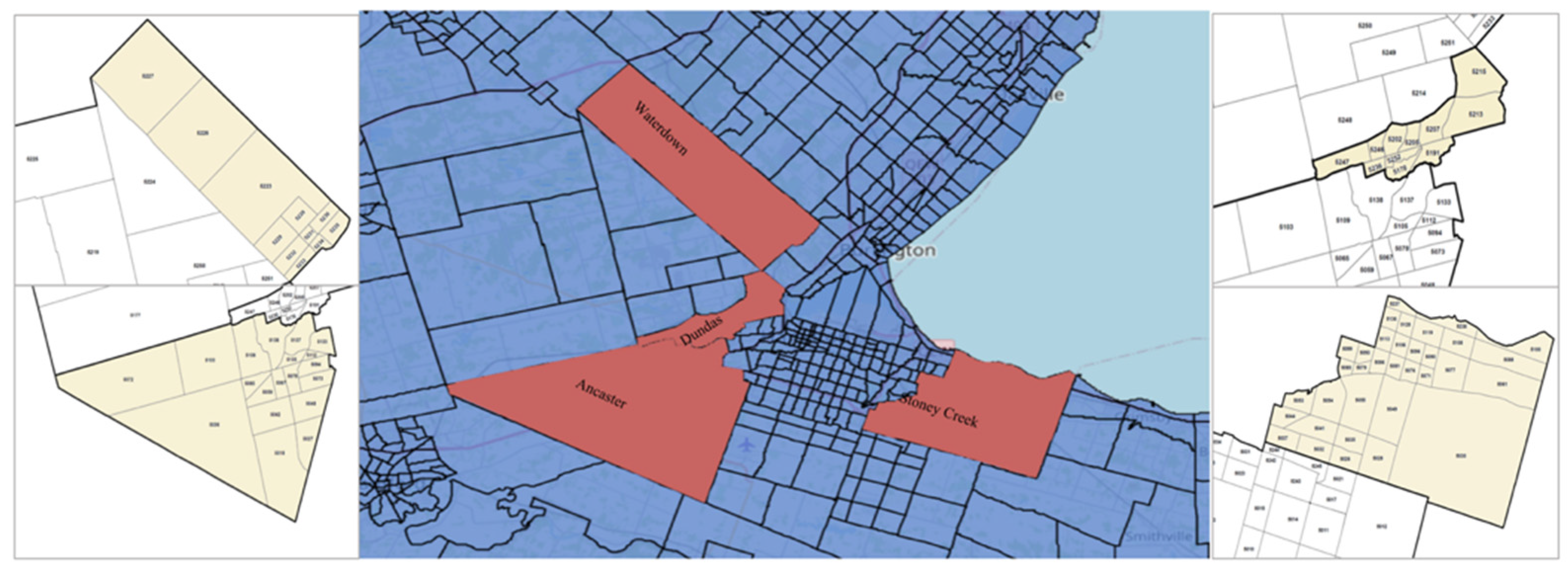
This study utilizes travel demand data extracted from the Transportation Tomorrow Survey (TTS), which provides comprehensive travel data in the Greater Golden Horseshoe Area in Ontario, Canada collected once every five years [44]. This study used the 2016 travel data for four suburban communities in the City of Hamilton: Waterdown, Dundas, Ancaster, and Stoney Creek (Figure 1,

Table 1. Demographics of Communities.

Community	Population	Area (km2)	Population Density (/km2)	Total Trips 1	Trips per Capita	Number of Intra-Community Trips	Share of Intra-Community Trips % 2
Waterdown	19,462	119	163.5	30,551	1.569	15,709	51.42
Dundas	24,285	23	1055.9	36,876	1.518	15,195	41.21
Ancaster	40,557	177	229.1	75,177	1.853	32,249	42.89
Stoney Creek	69,470	100	694.7	78,462	1.129	42,653	54.36

¹ Total Number of trips originating from the community to all TAZs in the Hamilton area (All modes). ² Percentage of trips inside the community of total trips originating from the community to all TAZs in the Hamilton area.

). The travel demand data was estimated at the TAZ level. TAZs represent areas from which and to which trips are allocated in a transport demand model. It should be noted that the 2021 TTS data are not yet available; in this study, we relied on the 2016 data.

The present study focused on intra-community travel demand data for these suburban communities in the City of Hamilton. Table 1 summarizes the demographics of the communities [45]. Waterdown and Dundas each consist of 11 TAZs, while Ancaster and Stoney Creek have 19 and 34 TAZs. The demand data show that almost half of all trips made within suburban areas are intra-community, for which a more sophisticated mode of transit may be required.

More specifically, this study focused on intra-community travel demand data for these communities as suburban regions in the City of Hamilton. For the purpose of this study, we extracted Origin–Destination trip matrices (O-D) for the intra-community trips within each community. Each matrix aggregates and represents only auto and transit trips with one-minute intervals for 24 h during a typical weekday in 2016. Trips performed with active modes of transportation were not included in our study.

Table 2. Travel mode shares in the communities.

	Waterdown		Dundas		Ancaster		Stoney Creek
Mode	Share of Trips (%)	Number of Trips	Share of Trips (%)	Number of Trips	Share of Trips (%)	Number of Trips	Share of Trips (%)	Number of Trips
Auto Driver	60.83%	9555	60.18%	9144	67.70%	21,834	65.77%	28,051
Auto Passenger	14.65%	2301	14.73%	2238	17.19%	5542	13.53%	5772
Public Transit	0.16%	26	0.35%	53	0.53%	172	0.51%	219
Active Transport	13.57%	2131	19.64%	2985	5.52%	1779	10.61%	4527
Other	10.8%	1696	5.10%	775	9.06%	2922	9.57%	4084
Total	-	15,709	-	15,195	-	32,249	-	42,653

displays the number and share of trips for each transportation mode across all communities. As shown in Table 2, in the target areas, public transport accounts for a small proportion of all trips made within the community. This confirms the need for complementary modes of transit in order to fulfill the existing intra-community travel demand. It is interesting that although the share of active transportation within suburban areas is considerable, it is not enough to compensate for the lack of a decent public transportation system. For active transportation, trips are made using non-motorized modes of travel based mostly on human physical activity. Other modes of travel (Table 2) may refer to any other modes not considered earlier, such as motorcycles, taxis, or school buses.

Figure 2a–d displays the demand distribution during a typical weekday in Waterdown, Dundas, Ancaster, and Stoney Creek. In all the communities under study, during the peak hours the share of active transportation in fulfilling the existing demand becomes significant. The considerable share of auto passengers over a typical weekday can provide valuable insight into the potential level of acceptance of ride-sharing within suburban communities.

3.2. Scenario Development and Assumptions

Four scenarios for the vehicle technology choices were investigated and compared: Internal Combustion Engine Vehicles (ICEV), Battery Electric Vehicles (BEV), and two Autonomous Electric Vehicle scenarios, one fully automated with no driver on board (AEV) and the other involving a safety attendant on board (AEV-2). The cost parameters for vehicles that are not yet available on the market were estimated based on existing data for similar vehicles. Each scenario considered serving the same demand for each community with a fleet of four different sizes: compact and full-size sedans, van, and minibuses, with a passenger capacity of three, six, nine, and fifteen passengers, respectively, in order to obtain the most efficient fleet composition.

This study used J-Horizon, a java-based vehicle routing problem software, in order to optimize the solution to the problem [46]. This platform provides a near-optimal solution to several versions of the vehicle routing problem, covering a wide range of details.

This software optimizes the cost of serving a known demand for a time interval using a fleet of shared mobility. It uses the jsprit library, which applies the ruin and recreate strategy to solve the vehicle routing problem with time windows [47]. This algorithm starts with an initial solution and improves the solution continuously until it meets specific criteria, indicating that the final solution is adequately near-optimal.

The output of the solution is a set of routes for the vehicles, the type and the number of the vehicles required for every five minutes, the chronology of serving the customers, and the cost of serving the requests along an optimized route for each vehicle. The approach of this study was to serve 100% of the potential demand in each region.

The demand data matrices for TAZs of Waterdown, Dundas, Ancaster, and Stoney Creek were used as the input for the software. A time resolution of five minutes was used to aggregate the demand data and to solve the routing problem [40]. Accordingly, vehicle availability was updated once every five minutes.

The model utilized the following conditions:

• Travel distances were all calculated in Manhattan format.
• The study focused on intra-community known travel demand data for each community. Therefore, the demand data only account for trips with an origin and destination located within the same community.
• Requests with the same pick-up and drop-off locations and time windows were aggregated. This was due to the high demand, especially during peak hours.
• A parking location was assumed to be at the center of the service area, the closest location to all TAZs of the region.
• According to the suburban nature of our case studies, an average travel speed of 45 kilometres per hour was utilized [40].
• The start of a time window for pick-up was calculated based on the distance between the parking and the pick-up locations, and the start time for customer drop-off was calculated based on the distance between pick-up and drop-off location.
• A 30% increase in the in-vehicle travel time as compared to the shortest route was accepted in this study in order to allow for sharing rides [4]; accordingly, for shared rides, vehicles were allowed to serve customers later compared to the time that was expected when the ride was not shared.
• The duration of each time window was three minutes.
• Driver cost was considered to be a fixed cost assigned to each vehicle. For this purpose, it was assumed that a vehicle was operated for an average of 19 hours on weekdays (based on the demand data) during an effective five-year lifespan of the fleet, with a driver cost of USD 15/hour. Although this rate is low, we assumed wages equal to the average salary of on-demand drivers (USD 15–20).
• Long-range electric vehicles were used, and as the average kilometres travelled per vehicle per day is less than the range of such vehicles, charging time during the day was not considered.
• The CO₂ emissions for conventional vehicles (ICEV) were based on tailpipe emissions, while for EVs and AEVs they were based on Well-to-Wheel emissions.
• A price premium of USD 18,000 to USD 40,000 was added incrementally to the purchase price of battery electric vehicles in variable sizes in order to estimate the price of autonomous vehicles not yet available on the market [32].

Specific early and late time windows were assigned for both pick-up and drop-off services; a passenger could not be picked up or dropped off sooner than early time windows, or be picked up or delivered later than late time windows (Equations (5)–(8)). The early time windows for drop-off were calculated based on the distance between pick-up and drop-off locations, multiplying by 1.3 (an acceptable increase in travel time). The duration of each time window was considered to be three minutes; therefore, late time windows were calculated by adding three minutes to the early time windows.

3.3. Methods

This study used a vehicle routing problem with time windows in which travel requests are serviced by a fleet of vehicles with various capacities. In a capacitated vehicle routing problem with time windows, the goal is to find optimal routes for multiple vehicles with limited carrying capacity, scheduling visits to customers who are only available during specific time windows [48]. In this study, the objective of the problem was to find a feasible set of routes to service all requests while minimizing the total cost of the service. A viable route for a vehicle started at a parking location and, based on the vehicle capacity, services a set of requests within the given time windows before ending back at the parking location. The parking location was assumed to be in the center of the service area, the closest location to all TAZs in the region. This location was used as a place where vehicles could wait until their next assignment. Although different depot locations will lead to different results, given that the area of each TAZ is quite small we believe that the impact of adding more depot locations in each TAZ would have only a marginal impact on the model outcome.

The following formulation was used to address the vehicle routing problem [49]. It is worth noting that diverse VRP algorithms can be used to address the study objectives [50,51,52], of which this study relied on the VRP mathematical formations utilized in J-Horizon. In order to define the problem in which n requests are serviced by m vehicles, K = {1, …, m}, two sets P = {1, …, n} and D = {n + 1, …, 2n} are used for pick-up and drop-off nodes. Each request is depicted by node i and i + n.

Vehicle k can serve a number of pick-ups and drop-offs, P_k ⊆ P and D_k ⊆ D. Since both pick-up and drop-off of a request are serviced by vehicle k, it is assumed that i ∈ P_k ⇔ i + n ∈ D_k. Let N = P ∪ D and N_k = P_k ∪ D_k. Then, t_k = 2n + k, k ∈ K and $t’$_k = 2n + m + k, k ∈ K depict the start and end parking location for each tour served by vehicle k.

Defining V = N ∪ {t₁, …, t_m } ∪ {$t’$₁, …, $t’$_m} as nodes and A = V × V as edges, there will be a directed graph G = (V,A). A sub-graph G_k = (V_k,A_k) can be defined for each vehicle, where V_k = N_k ∪ {t_k} ∪ {$t’$_k} and A_k = V_k × V_k. Each edge (i, j) ∈ A has a distance measure of d_ij ≥ 0 and a travel time of t_ij ≥ 0.

There is a time window (a_i,b_i) for each node i ∈ V. Each node needs to be visited within its time window. For each node i ∈ N, l_i is defined as the load that the respective request will add onto the vehicle with a specified capacity C_k; thus, l_i ≥ 0 for i ∈ P and l_i = −l_i−n for i ∈ D. П_i is a precedence number assigned to each node which defines the priority of visiting that node. For each vehicle k, an admissible route $\overline{r}$ starts from parking location t_k to its destination parking location, $t’$_k:

$$\overline{r}=(t_k=v_1,v_2, ..., v_h={t’}_k)$$

(1)

while satisfying the precedences, time windows and the capacity constraints. Each vehicle should visit only the nodes which could be serviced by that vehicle. Equations (3) and (4) ensure that for each request, both pick-up and drop-off are served by the same vehicle, considering that the pick-up takes place before the drop-off.

v_i ∈ N_k, i = 2, …, h − 1

(2)

i ≤ j, v_i ∈ P_k, v_j ∈ D_k, v_j = v_i + n

(3)

i ≤ j, П_vi ≤ П_vj

(4)

Si ∈ R₀⁺ is defined to represent the time when a vehicle starts the service at node $v_i$. In other words, $S_1$ and $S_h$ represent the time for serving demands in the first and the last nodes, respectively. In addition, each node needs to be visited within its time window. With this definition, Equations (5)–(8) ensure that the service takes place within the time windows:

a_vi ≤ S_i ≤ b_vi, i = 1, …, h

(5)

S_i+1 ≥ S_i + t_{vi, vi+1}, i = 1, …, h − 1

(6)

$$a_{t_k}\le S_1 \le b_{t_k}$$

(7)

$$a_{{\acute{t}}_k}\le S_h \le b_{{\acute{t}}_k}$$

(8)

Equations (9)–(12) check the capacity constraint for vehicles along the tours/routes. L_i ∈ R₀⁺ denotes the load of the vehicle at node i after serving node i.

L_i ≤ C_k, i = 1, …, h

(9)

L_i+1 = L_i + l_i+1, i = 1, …, h − 1

(10)

L₁ = 0

(11)

L_h = 0

(12)

Finally, the cost of route $\overline{r}$ is:

$$c_{\overline{r}}=\sum _{i=1}^{h-1}{d}_{v_i,v_{i+1}}$$

(13)

One service from a given vehicle in shared mobility may include several nodes, each of which may have different demands, considering the vehicle capacity. The total cost of this route can be calculated by summing the costs of travelling between each of these nodes. The problem is formulated as follows: R is defined as the set of all feasible routes. For $\overline{r}$ ∈ R, (${\alpha }_{j\overline{r}}$) is a boolean matrix indicating whether or not route $\overline{r}$ is used to service request j. (${\beta }_{k\overline{r}}$) is also a boolean matrix that shows whether vehicle k carries out route $\overline{r}$. A binary variable $x_{\overline{r}}$ indicates the presence of route $\overline{r}$ in the solution:

$$\mathit{min}f(x)= {\sum }_{\overline{r}\in R }{c}_{\overline{r}}{x}_{\overline{r}}$$

(14)

$$s.t. {\sum }_{\overline{r}\in R }{\alpha }_{j\overline{r}}{x}_{\overline{r}}=1 j=1, ..., n$$

(15)

$${\sum }_{\overline{r}\in R }{\beta }_{k\overline{r}}{x}_{\overline{r}}=1 k=1, ..., m$$

(16)

$$x_{\overline{r}} \in \{\mathrm{0}, \mathrm{1}\} \overline{r}\in R$$

(17)

3.4. Cost Parameters

Cost parameters were defined and calculated for all vehicle sizes and powertrain technologies. These parameters were based on the vehicles available on the market. The cost parameters include purchase price and tax (Ontario tax rate of 13% HST), maintenance and repair for five years, driver cost for five years, licensing and registration, insurance for five years, energy (fuel/electricity) consumption, CO₂ emission damage costs (

Table 3. Cost Parameters (USD).

	Technology	Purchase & Tax ($) 1	Maintenance and Repair ($)	Driver ($)	License & Registration ($)	Insurance ($)	Energy ($/km) 2	CO2 ($/km)
3-seater	ICEV	29,100	2550	364,650	510	7350	0.0604	0.0102
	BEV	38,600	2550	364,650	510	7350	0.0142	0.0003
	AEV	59,400	2550	0	510	7350	0.0142	0.0003
	AEV-2	59,400	2550	255,250	510	7350	0.0142	0.0003
6-seater	ICEV	29,500	2950	364,650	510	7350	0.0986	0.0166
	BEV	42,800	2950	364,650	510	7350	0.0184	0.0004
	AEV	71,900	2950	0	510	7350	0.0184	0.0004
	AEV-2	71,900	2950	255,250	510	7350	0.0184	0.0004
9-seater	ICEV	38,200	3650	364,650	510	7350	0.1735	0.0262
	BEV	74,800	3650	364,650	510	7350	0.0288	0.0006
	AEV	112,200	3650	0	510	7350	0.0288	0.0006
	AEV-2	112,200	3650	255,250	510	7350	0.0288	0.0006
15-seater 3	ICEV	36,600	4400	364,650	510	7350	0.0438	0.0180
	BEV	83,100	4400	364,650	510	7350	0.0288	0.0006
	AEV	128,800	4400	0	510	7350	0.0288	0.0006
	AEV-2	128,800	4400	255,250	510	7350	0.0288	0.0006

¹ Retail price plus 13% tax. For vehicles not available on the market, a similar vehicle was used as a reference to estimate the price [57]. ² Energy cost was calculated for one kilometre of operation considering the fuel economy in litres per km for conventional vehicles and kWh per km for electric vehicles. ³ A diesel-based vehicle was selected for the 15-seater option, and therefore the operation cost (fuel economy) and the associated emissions are lower than for their petrol counterpart.

). All costs are indicated in United States Dollars. The cost parameters for vehicles that are not yet available in the market were estimated based on the data for similar vehicles. For example, the cost of AEVs was estimated by considering an added premium for electric propulsion and autonomous technologies. This approach, suggested by Quarles et al. (2020), uses a conservative estimation for the added cost of delivering a fully autonomous (level 5) vehicle [53].

The cost of CO₂ emission reflects the damage costs and impacts of CO₂ on human health, climate, and natural and artificial systems [54]. For conventional vehicles, this value is reported by the manufacturer as gr/km CO₂ emission. For electric vehicles, it was calculated based on CO₂ emissions associated with electricity generation, known as the annual Average Emission Factor (AEF), which is 31 gr CO₂eq per kWh for Ontario [55]. This study considered the CO₂ damage costs as calculated by Noori et al. (2015) based on a number of factors [56]. A unit damage cost of 0.06 dollars per kilogram was inferred, with values adjusted considering the inflation rate. All data reported in Table 3 are based on actual vehicles on the market; the selection of the vehicles was based on the best-sold vehicle in each category.

The maintenance costs were estimated based on the suggested maintenance schedule for the available vehicles or an estimation based on the available information on the market. The maintenance costs for AEVs were assumed to be the same as those for conventional vehicles [42]. The insurance costs for the vehicles depended on a variety of parameters including vehicle type, location, and driver specifications. An annual cost of USD 1470 was estimated for all types of vehicles in this study [58].

Because autonomous vehicles of different sizes are not widely available, there are no solid data regarding their capital costs. ENO (2013) estimates price premiums [53] of USD 25,000 to USD 50,000 for vehicle autonomy technology, which could decrease to USD 10,000 in ten years [32]. Loeb et al. (2019) assume a price premium of USD 5000 to USD 25,000 for the vehicles [42]. In this study, a price premium of USD 18,000 to USD 40,000 was considered for vehicles with capacities of 3, 6, 9, and 15 passengers incrementally.

One of the most significant cost parameters considered in this study was driver cost, as this represents the biggest savings for a fully autonomous scenario and is where autonomous technology choice compensates for its large purchase costs. To take into consideration the cost of the driver, a fixed driver cost of USD 285 per day was assigned to each vehicle, considered as a minimum in order to provide a baseline. For the AEV-2 scenario, considering a minimum hourly rate of payment for the same hours of work per day as for drivers, a fixed cost of USD 196 per day was assigned to each vehicle in order to consider the safety attendant cost. Except for energy consumption and emission costs, which were indicated in dollars per kilometre, the cost parameters were calculated for an effective period of five years of employment in a shared fleet. By assuming a lifespan of around 250,000 kilometres for vehicles [59], these costs were then illustrated in terms of dollar per kilometre value and used as the input for each type of vehicle in the optimization problem.

For all three electric vehicle scenarios (BEV, AEV, and AEV-2), a charging infrastructure cost of 0.0041 dollars per kilometre was considered in the total cost per day based on the kilometres travelled [40].

4. Results

A summary of the results of the optimization for each scenario for 24 h of weekday travel demand data is shown in

Table 4. Summary of the Results.

Context	Scenario	Cost ($)/day	Cost ($)/km	Cost ($)/Passenger	VKT 1	Occupied VKT	CO2 (ton)	CO2/km 2	Occupancy (%)
Waterdown	ICEV	28,452	1.71	2.39	16,593	4432	4.907	296	22.32
	BEV	30,744	1.87	2.58	16,460	4344	0.158	9.6	23.99
	AEV	9363	0.57	0.79	16,561	4448	0.155	9.36	24.05
	AEV-2	26,617	1.59	2.24	16,731	4512	0.155	9.26	23.97
Dundas	ICEV	12,983	1.71	1.14	7575	3521	2.212	292	39.56
	BEV	14,015	1.84	1.23	7598	3561	0.069	9.08	42.55
	AEV	4213	0.55	0.37	7608	3555	0.069	9.07	42.69
	AEV-2	12,048	1.60	1.06	7541	3537	0.069	9.15	42.69
Ancaster	ICEV	73,353	1.71	2.66	42,953	16,465	12.626	294	32.04
	BEV	79,088	1.85	2.87	42,692	16,029	0.397	9.3	33.65
	AEV	24,383	0.56	0.88	43,364	16,551	0.402	9.27	33.87
	AEV-2	68,183	1.59	2.47	42,934	16,578	0.399	9.29	33.82
Stoney Creek	ICEV	97,249	1.71	2.84	56,758	16,458	16.460	290	25.32
	BEV	104,293	1.84	3.05	56,615	16,486	0.517	9.13	27.29
	AEV	31,401	0.55	0.92	56,856	16,556	0.520	9.15	27.30
	AEV-2	89,242	1.57	2.61	56,692	16,496	0.519	9.15	27.35

¹ Vehicle Kilometers Travelled. ² 10 × 10⁻⁶ ton CO₂ per kilometer.

. Here, occupancy% represents the percentage of occupied seats in a vehicle during all trips during a five-year interval.

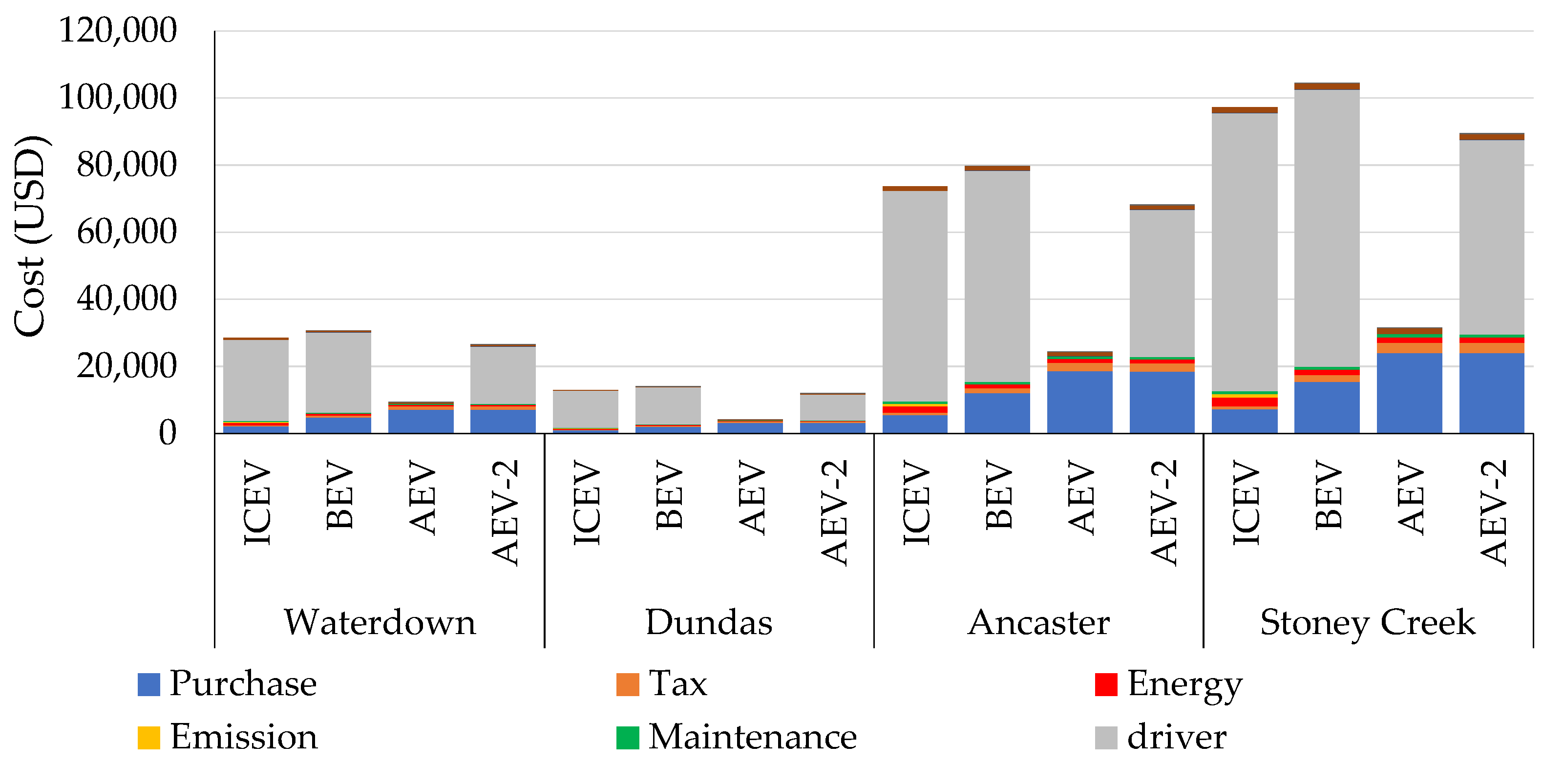
The results suggest that the shared mobility can be offered at the price of USD 1.71, 1.87, 0.57, and 1.59 per kilometre of operation in Waterdown, USD 1.71, 1.84, 0.55, and 1.60 per kilometre in Dundas, USD 1.71, 1.85, 0.56, and 1.59 per kilometre in Ancaster, and USD 1.71, 1.84, 0.55, and 1.57 per kilometre in Stoney Creek for ICEV, BEV, AEV, and AEV-2 scenarios, respectively (Figure 3). Overall, the results indicate that for all four target communities AEV would be the most efficient shared mode of travel, followed by AEV-2, ICEV, and BEV, respectively. The reason that automated forms of shared mobility are associated with the lowest costs lies in the fact that they can lower operational costs by eliminating driver wages, which eventually leads to lower fares for users. Overall, it is safe to say that employing autonomous vehicles in a shared fleet could counteract the negative aspects of autonomy (e.g., high initial costs). It is interesting that in the short term, shared modes of travel with battery-electric powertrain were found to be less efficient than ICEVs due to their higher fixed costs; however, the lower energy and environmental costs may compensate in the long term.

According to the results, the cost of running a fleet of AEVs in Waterdown is about 33%, 30%, and 35% of the cost of choosing ICEV, BEV, and AEV-2 fleet. These shares are about 32%, 30%, and 35% in Dundas, 33%, 31%, and 36% in Ancaster, and 32%, 30%, and 35% in Stoney Creek, respectively (Figure 4). While the ICEV scenario represents a costly scenario and AEV depicts an ideally cost-efficient scenario, AEV-2 portrays a more realistic scenario of the autonomous fleet cost in the near future. The cost of the AEV-2 scenario is less than the other two non-autonomous scenarios, with smaller savings compared to AEV.

The Vehicle Kilometers Travelled (VKT) does not differ noticeably for ICEV, BEV, AEV, and AEV-2. The results suggest that the costs of running the fleet in all four areas are comparable, while the Battery Electric fleet is predicted to introduce the highest per-kilometre cost of USD 1.84–1.87, and the Autonomous Electric fleet represents the lowest of such costs, i.e., USD 0.55–0.57. The average cost per-passenger is consistently the lowest in Dundas and the highest in Stoney Creek, which can be attributed to their respective shares of intra-community trips.

There is a considerable difference in the consequent CO₂ emissions of conventional and electric vehicles (Figure 5). This measure for conventional vehicles is 4.9, 2.2, 12.6, and 16.5 tons for a day of operation in Waterdown, Dundas, Ancaster, and Stoney Creek based on tailpipe emission, and as expected is much higher than the emissions for electric vehicle operation calculated based on emissions factors for electricity generation.

As displayed in Figure 6, the results for all case studies suggest that the fleet composition is almost the same when using the BEV, AEV, or AEV-2 fleets. The composition is different for the ICEV fleet as the optimized solution excludes midsize vehicles with six and nine passengers. This is due to a disproportionate increase in the price of available ICEVs in the market which makes the cost of midsize vehicles relatively close to larger vehicles and impedes the competitiveness of midsize vehicles in this category with larger ones. The total fleet size is slightly smaller in the ICEV scenario. In all four scenarios, 15-seater vehicles constitute the majority of the fleet. In addition, the number of 15-seater vehicles in the ICEV scenario is on average 21%, 12%, 9%, and 9% higher than the number of 15-seater vehicles in the other three scenarios in Waterdown, Dundas, Ancaster, and Stoney Creek, respectively.

The Utilization rate is a measure for reflecting the efficiency of fleet operation in terms of utilizing resources. Utilization rates are calculated based on the time that each vehicle is idle and waiting in parking with no assigned request (including occupied and unoccupied trips). Utilization rates excluding the time that it takes an empty vehicle to reach a pick-up location or get back to the parking location, that is, including only occupied trips, are included as well. The data show no demand for the hours after midnight. Therefore, this duration is excluded from calculating the Utilization rates.

Table 5. Utilization and Idling Rates (%).

		3-Seater	6-Seater	9-Seater	15-Seater	Fleet Total
Waterdown
ICEV	Occupied and unoccupied 1	21.99	-	-	39.87	38.57
	Occupied 2	4.98	-	-	8.89	8.61
	Idling Rate	78.01	-	-	60.13	61.43
BEV	Occupied and unoccupied	20.20	27.19	26.15	41.65	36.85
	Occupied	3.69	6.43	5.93	10.42	9.00
	Idling Rate	79.8	72.81	73.85	58.35	63.15
AEV	Occupied and unoccupied	23.14	27.60	28.12	40.15	36.59
	Occupied	4.75	6.49	6.16	8.96	8.15
	Idling Rate	76.86	72.4	71.88	59.85	63.41
AEV-2	Occupied and unoccupied	18.04	26.78	30.71	40.18	35.27
	Occupied	6.48	6.00	7.41	8.68	8.05
	Idling Rate	81.96	73.22	69.29	59.82	64.73
Dundas		3-seater	6-seater	9-seater	15-seater	Fleet Total
ICEV	Occupied and unoccupied	16.18	-	-	20.87	20.50
	Occupied	5.02	-	-	8.08	7.84
	Idling Rate	83.82	-	-	79.13	79.50
BEV	Occupied and unoccupied	15.16	14.68	14.61	20.39	19.15
	Occupied	5.10	5.42	5.77	8.00	7.42
	Idling Rate	84.84	85.32	85.39	79.61	80.85
AEV	Occupied and unoccupied	16.33	16.33	12.35	20.32	19.21
	Occupied	5.55	6.00	4.59	7.97	7.42
	Idling Rate	83.67	83.67	87.65	79.68	80.79
AEV-2	Occupied and unoccupied	16.5	15.56	14.66	20.34	19.35
	Occupied	5.72	6.20	6.05	7.90	7.51
	Idling Rate	83.5	84.44	85.34	79.66	80.65
Ancaster		3-seater	6-seater	9-seater	15-seater	Fleet Total
ICEV	Occupied and unoccupied	30.02	-	-	44.89	43.77
	Occupied	10.98	-	-	15.63	15.28
	Idling Rate	69.98	-	-	55.11	56.23
BEV	Occupied and unoccupied	29.54	35.43	34.1	43.90	41.72
	Occupied	10.72	11.74	12.09	15.20	14.46
	Idling Rate	70.46	64.57	65.9	56.10	58.28
AEV	Occupied and unoccupied	31.36	35.00	30.67	44.22	41.77
	Occupied	11.20	12.32	10.54	15.97	15.02
	Idling Rate	68.64	65.00	69.33	55.78	58.23
AEV-2	Occupied and unoccupied	30.00	37.78	34.09	43.92	41.97
	Occupied	11.02	12.76	11.96	15.46	14.77
	Idling Rate	70.00	62.22	65.91	56.08	58.03
Stoney Creek		3-seater	6-seater	9-seater	15-seater	Fleet Total
ICEV	Occupied and unoccupied	32.21	-	-	30.42	30.55
	Occupied	6.41	-	-	7.020	6.98
	Idling Rate	67.79	-	-	69.58	69.45
BEV	Occupied and unoccupied	34.75	27.93	28.52	29.20	29.44
	Occupied	7.02	7.42	6.05	6.74	6.76
	Idling Rate	65.25	72.07	71.48	70.80	70.56
AEV	Occupied and unoccupied	35.63	25.16	27.40	29.31	29.32
	Occupied	7.09	6.80	5.97	6.77	6.75
	Idling Rate	64.37	74.84	72.6	70.69	70.68
AEV-2	Occupied and unoccupied	37.52	30.13	27.44	29.51	29.90
	Occupied	7.42	7.92	5.77	6.83	6.87
	Idling Rate	62.48	69.87	72.56	70.49	70.10

¹ Considers the whole time that a vehicle is being used to serve customers (includes empty trips to and from customers). ² Considers only the time that a vehicle is occupied and is being used to serve customers (excludes empty trips).

displays the Utilization rates based on the two aforementioned definitions.

The idling rate accounts for the time that vehicles are idle or parked waiting for a request. Dundas has the highest idling rate for all vehicles sizes and types of powertrain technologies. This result is attributed to the fact that Dundas has the lowest number of intra-community trips per population in each ${\mathrm{km}}^2$ area among the four target communities. In contrast, the idling rate of fleets in Ancaster is the lowest, as Ancaster has the highest number of intra-community trips per population in each ${\mathrm{km}}^2$ area.

It is noteworthy that a large difference between the demand at peak and off-peak hours, as shown previously in Figure 2, demands additional vehicles within specified time windows, which consequently increases the number of idle vehicles during off-peak hours. The idling cost impacts the total cost of ownership, especially under a regulated service model. However, such an impact might be mitigated under a private-partnership business model.

Additionally, a sensitivity analysis is used (

Table 6. OLS Model outcomes.

	Coefficients	Std Err	Standardized Coefficients	t-Statistic	P > |t|	[0.025	0.975]
Trips/Capita	14.3443	0.988	0.562	14.513	0.005	10.092	18.597
Trips/km2	0.0134	0.002	0.979	8.162	0.015	0.006	0.02

) to determine how the utilization rate is affected based on changes in its potential input variables. In this regard, we utilized Ordinary Least Square (OLS) to model the relationship between utilization rate and its contributing factors, including Trips/Capita and Trips/km². The results confirm that there is a strong positive relationship between the target values and both parameters of Trips/Capita and Trips/km² (${\mathrm{R}}^2$ and Adj.${ \mathrm{R}}^2$ equal to 0.998 and 0.997, respectively). According to the obtained standardized coefficients, an increase in Trips/Capita by 1 standard deviation increases the utilization rate by 0.562 standard deviations, while increasing Trips/km² by 1 standard deviation results in an increase of 0.979 standard deviations. This shows that Trips/km² is considerably more effective than Trips/Capita in terms of the rate of utilization.

5. Discussion and Conclusions

This study provides insights for policymakers, service providers and researchers on the potential costs and benefits of considering shared mobility options, using quantitative measures and implications in order to assess shared service in a suburban context. The results indicate that approximately 2.1 to 3.9 vehicles are required per 1000 residents in each area to serve demand using shared mobility, which represents a significant reduction in fleet size if considered as a replacement for private cars. These results are similar to those of a previous study by Kroger et al. (2017) addressing 2.5–4 vehicles per 1000, which illustrate that although system efficiency in terms of fleet size is higher in urban areas, suburban areas are not excluded from the corresponding benefits [11].

The results of optimization for the suburban regions under study suggest a similar fleet composition when using a fleet of shared BEV AEV, or AEV-2 in which the fleet is dominated by larger vehicles with capacity for fifteen passengers. The unproportioned increase in the price of midsize ICE vehicles, however, excludes midsize vehicles in this scenario and raises the share of 15-seater vehicle capacity to 98.5%, 98.3%, 98.4%, and 98.5% for Waterdown, Dundas, Ancaster, and Stoney Creek, respectively.

The largest portion of the costs of serving the demand for vehicles is to the driver cost, which represents about 85% and 79% of the total cost for ICEV and BEV scenarios in each community. This is despite using a very low driver rate (USD 15) in the model. Eliminating the driver cost in the AEV scenario not only compensates for the much higher purchase price of Autonomous vehicles, but leads to 67.1% and 69.5% lower total costs compared to a fleet of ICEV and BEV for Waterdown, 67.5% and 69.9% lower total costs in Dundas, 66.8% and 69.2% lower costs in Ancaster, and 67.7% and 69.9% lower costs in Stoney Creek.

The results suggest that the costs of running the fleet in all four areas are comparable, while the Battery Electric fleet is predicted to introduce the highest per-kilometre cost at USD 1.84–1.87, and the Autonomous Electric fleet represents the lowest of such costs, i.e., USD 0.55–0.57. Fleet average cost per passenger is consistently the lowest in Dundas and the highest in Stoney Creek. The suggested costs per kilometre and costs per passenger for the operation of a fleet of shared vehicles in each region should be contemplated in the context of a suburban region in which the longest distance is around 20 km.

The results for the four scenarios illustrate that in comparing the Utilization rates of vehicles, none of the scenarios excels tremendously in terms of efficiency; with the highest Utilization rates being 42%, 21%, 45%, and 31% for Waterdown, Dundas, Ancaster, and Stoney Creek, respectively. The rates are almost the same for all scenarios and less than would be expected for an efficient fleet of shared vehicles if the target were adequately serving the whole demand. This may be addressed by cutting down the fleet during off-peak hours of the day.

Overall, this study perceives potential benefits in adopting shared mobility services in the target suburban regions when utilizing an autonomous electric fleet, with pursuant savings in total costs and emissions. In the absence of operationally safe Autonomous Electric Vehicles, the more conservative scenario of employing a fleet of shared Autonomous Electric Vehicles with the presence of safety attendants could result in 6–8% and 13–14% savings compared to a shared fleet of conventional and Battery Electric Vehicles, respectively.

However, it is worth noting that these recommendations do not consider the potential changes in user perception towards different technologies (i.e., fully autonomous), nor the resultant changes in mode choice. Therefore, it should be clear to the readers that the results of this study could be generalized if there are no major shifts in mode choice due to the advent of fully autonomous vehicles. Such a disruptive technology will indeed cause a paradigm shift in mode choice and in transit provision at large. These topics provide avenues for future research studies.