Abstract
Tourism development consumes ecological resources to varying extents while bringing economic benefits; tourism eco-efficiency (TEE) assessment has thus become an area of major focus in destination sustainability research. This paper intends to examine the spatiotemporal characteristics and driving factors of eco-efficiency changes in 36 tourist cities on the Chinese mainland from 2010 to 2019, using a super-slacks-based measure (SBM) model, the data envelopment analysis (DEA)–Malmquist index, spatial correlation, and regression analysis. In contrast to the previous work, this work explores TEE among major tourist cities in China by considering the undesirable outputs of carbon emissions and sewage. The results show that (1) the TEE of most cities during the study period was low but increasing; there were significant spatial differences among different cities, and the eco-efficiency of the same city fluctuated over time. (2) The TEE was globally uncorrelated, but low-eco-efficiency areas were adjacent to each other and formed agglomerates, enhancing the negative spillover effect. (3) Despite fluctuations, the Malmquist indices exhibited positive trends, which resulted from the technical progress index rather than the technical efficiency index. (4) Socioeconomic development significantly promoted TEE. This research reveals the evolutionary law of TEE on the urban scale and explores the impact of social and economic development on TEE, which can provide a reference for policymaking and enrich research on destination sustainability.
1. Introduction
The rapid development of the tourism industry has brought enormous economic benefits to society but has also caused devastating ecological damage, as the blind pursuit of economic benefits has inevitably generated serious ecological and environmental problems [1,2,3]. Tourism activities consume a large amount of energy and natural resources, resulting in air pollution, water pollution, solid waste pollution, and carbon dioxide emissions, all of which threaten the environmental quality of the tourism destinations [4,5]. An increasing number of researchers have found that the goods and services involved in tourism have overturned the traditional concept of tourism as an “industry with low energy consumption, low pollution, and low emission” [6]. Thus, it has become a top priority to objectively recognize the existing and possible environmental problems of the booming tourism industry, to strive to balance economic development and environmental protection, and to achieve the sustainable development of tourism [7].
China is the East Asia–Pacific’s largest tourism and travel economy; it has the highest index for natural and cultural resources but faces hurdles when attempting to achieve environmental sustainability [8]. The Chinese government has therefore emphasized that tourism development should take both efficiency and quality into consideration [9]. However, achieving coordination between the rapid development of the tourism industry and ecological environment protection poses challenges. How to correctly grasp the impact of tourism development on the ecological environment and coordinate the relationship between the economic benefits and the ecological costs are key issues facing the academic community [10].
To evaluate the state of the trade-offs between economic benefit and environmental degradation, the concept of “eco-efficiency” has emerged in the sustainable development fields. Eco-efficiency is a management strategy based on the concept of creating more goods and services while using fewer resources and creating less waste and pollution [11]. In 2005, Gosling introduced ecological efficiency into tourism research for the first time and conducted quantitative analysis on the economic value and environmental impact of tourism [12]. TEE is a key indicator used to measure the green development speed of tourism. Its main objective is to create the highest economic benefits with the lowest environmental costs. It has become an important strategic tool for assessing the sustainable development of tourism [13]. Research on TEE focuses mainly on the connotations of eco-efficiency and destination management and the measurement, influencing factors, and application of eco-efficiency [14,15,16,17,18,19]. The main research methods include the single ratio method [20,21,22,23,24,25], the ecological footprint method [26], the carbon footprint method [27,28,29,30,31], the water footprint method [32,33,34,35,36,37], and the data envelopment analysis (DEA) model [38,39,40,41].
The main modeling method is the DEA model proposed by American operations research scientist Charnes et al. [22]. The traditional DEA model considers only the proportion of change in the input–output variables and does not consider the relaxation of the input–output variables, thus leading the measured value to be higher than the actual value [42]. To address this concern, the slacks-based measure (SBM) model was developed [43]. The SBM model not only includes the unexpected output in the model but can also address the relaxation of the input–output variables in the traditional DEA model. However, the original scale information of the efficiency boundary projection value is also lost, resulting in a relatively low calculation result by the model. To enable the SBM model to compare multiple decision-making units (DMUs) with relatively effective efficiency, Tone proposed a super-SBM model combining the super efficiency DEA model and the SBM model in 2002 [44]. In the process of tourism industry development, it is generally expected that the less the ecological pollution caused by tourism activities, tourism transportation, accommodation facilities, and other related industries and activities the better; that is, it is better to minimize the unexpected output of the tourism industry. To overcome the defect of the fact that DMUs with the same efficiency value cannot be compared in the SBM–DEA model, this paper chooses the super-SBM model with a non-guidance angle for research.
Many scholars have studied the ecological efficiency of tourism from multiple perspectives. Wang [45] took 31 provinces in China as an example, measured the ecological efficiency of 31 provinces from 1997 to 2016 by using the unexpected output model, and analyzed the spatial and temporal evolution trend and pattern of ecological efficiency in the past 20 years. The panel Tobit regression model and the geographical detector model were used to explore the internal and external driving forces of the tourism ecological economic system. Based on the panel data of China’s Yangtze River Delta and Pearl River Delta and the Beijing–Tianjin–Hebei urban agglomerations from 2008 to 2017, Sun [46] used the super-EBM mixed distance model to measure the tourism ecological efficiency of 63 cities. The external factors were analyzed by a panel regression model. Li [47] used the SBM undesirable output model of DEA to measure the ecological efficiency and spatial autocorrelation of 28 national forest parks to analyze their spatial and temporal evolution. Castilho et al. [48] reviewed the impact of tourism on the overall ecological efficiency of 22 Latin American and Caribbean countries from 1995 to 2016. The DEA method is used to calculate the overall ecological efficiency of various countries, and the panel autoregressive distribution lag model is used to analyze the impact of tourist sources, tourism capital investment, and the direct contribution of tourism employment on ecological efficiency. Studies on the ecological efficiency of small-scale tourism destinations have also gradually emerged [49,50,51]. For example, based on the ecological efficiency model, Hu [52] creatively proposed the tourism ecological welfare index and accordingly analyzed the change trend and driving effect of tourism ecological welfare in Changzhou from 1995 to 2017, aiming to provide a new perspective for evaluating the tourism industry’s capacity for green and sustainable development.
Although previous studies on TEE contributed to the advancement of destination sustainability research, they have the following limitations. First, TEE is often compared among countries or regions, failing to assess the tourism efficiency on a fine scale. Second, due to the different levels of tourism development, the selected DMUs lack comparability, which affects the general conclusions. Third, less attention has been given to the structural evolution mechanism of TEE. These research gaps leave a series of open questions: are there significant differences in TEE between cities with similar levels of tourism development? What is the law of its spatiotemporal evolution? What factors are driving this pattern of change? To answer the questions above, this study selects 36 tourist cities in China with different economic development levels, geographical locations, and resource endowments. Based on the “bottom-up” accounting method of carbon emissions and wastewater emissions, a multi-input and multi-output index system is constructed by using the super-SBM model and the DEA–Malmquist index to comprehensively reflect the ecological efficiency of tourism. The tourism ecological efficiency of 36 tourist cities in China is strictly evaluated by using this system. In addition, ArcGIS is used to analyze the spatial evolution pattern and correlation, and cluster analysis is used to explore the ecological efficiency correlation among the tourist cities. Finally, the paper discusses the impact of social and economic development on TEE by using regression analysis. This study aims to deepen the understanding of destination sustainability and to put forward strategies for high-quality tourism development by examining the status and evolution of eco-efficiency in China’s tourist cities. The paper is structured as follows: Section 2 provides the study methodology, including the models and data sources; Section 3 gives the results and analysis; Section 4 is the discussion; and Section 5 is for the conclusions.
2. Materials and Methods
2.1. Methods
2.1.1. Super-SBM Model Based on Undesirable Outputs
Tone’s super-SBM model [44] is selected for the static calculation of ecological efficiency. The specific model formula is constructed as follows:
where is the TEE; m, are the numbers of inputs, desirable output indicators, and undesirable output indicators, respectively; are the input slack, the desirable output slack, and the undesirable output slack, respectively; and λ is the weight vector. ≥ 1 and < 1 indicate that the evaluated DMU is relatively effective and ineffective, respectively.
2.1.2. “Bottom-up” Calculation of Carbon Emissions
Emission accounting methods for tourism can be divided into two main categories: “bottom-up” and “top-down” [53]. Wang et al. [54] argued that China has not yet established a systematic tourism satellite account and greenhouse gas emission monitoring system. Considering that the 36 cities investigated in this study are from different provincial regions, a “bottom-up” method for carbon emission calculation is selected:
where , , and are the emissions of tourism transport, accommodation, and activities in region (g), respectively. denotes passenger turnover volume with the type-x transport mode; represents the proportion of tourists using the type-x transport mode; and is the emission factor for the type-x transport mode. A previous study [55] showed that for highways, civil aviation, railways, and waterways, the f values are 0.138, 0.647, 0.316, and 0.106, respectively, and the corresponding values are 133, 137, 27, and 106 g CO2/p km, respectively. denotes the number of beds in tourist hotel rooms, is the average occupancy rate of tourist hotel rooms in the region, and is the emission factor per bed per night (g/p visitor-night), which takes a value of 2.458 [30]. denotes the number of tourists performing a type-s tourism activity in the region, and is the corresponding emission factor. The emission factors for sightseeing tourism, business tourism, leisure tourism, family tourism, and other types of tourism activities are 417, 1670, 786, 591, and 172 g CO2/p visitors, respectively [55].
2.1.3. Correlation Analysis
- (1)
- Global spatial autocorrelation is measured using the global Moran index I, which can reflect the correlation of each regional unit in the study area with its neighboring regional units [26]. The equation is as follows:where and are the observed values in regions and , respectively is the mean; is the spatial vector matrix; and is the total sample size. The value range for is [−1, 1], and indicate negative and positive correlations, respectively, and the closer I is to 0, the weaker the correlation is.
- (2)
- The Moran index measures the correlation between spatial units but cannot fully reflect the specific characteristics of such correlations. Local spatial autocorrelation can be used to characterize the spatial distribution of the clustered similarity of regional units [26]. The equation is as follows:where positive and negative values of indicate that the similarity of local spatial units tends to be spatially clustered and dispersed, respectively.
2.1.4. Malmquist Model
The super-SBM model of undesirable outputs can compare the relative efficiency of the DMUs within a group only, and thus, it is a static analysis and fails to consider dynamic changes in efficiency when using panel data. To analyze the dynamic changes and decomposition of TEE, total factor productivity (TFP) can be decomposed into the technological change (TC) index and the technological efficiency (TEC) index, and the TEC index can be further decomposed into the pure TEC (PTEC) index and the scale efficiency (SEC) index [54,56] with the following equations:
where and are the input–output data for periods and , respetively. When the index values derived from Equation (5) are greater than 1, it indicates an increase in TEE and other decomposed parameters from period t to period ; values less than or equal to 1 indicate that these indicators are declining.
2.1.5. Cluster Analysis
Cluster analysis is a process of dividing all objects in a study area into several classes based on similarity. Cluster analysis methods include hierarchical clustering, k-means clustering, decomposition, addition, and dynamic clustering. This study uses the k-means method to classify the TEE of China’s 36 tourist cities and visually reflect their similarities and differences regarding eco-efficiency.
2.2. Composition of the Indicator System
The 36 cities investigated in this study have different administrative levels, and the statistical yearbooks, statistical bulletins, and relevant statistical data for each city may not contain the same data, thus leading to missing data for the study. In addition, deriving an estimate of the relevant data (e.g., emissions of the “three wastes of tourism” in each city) by distributing questionnaires in the 36 cities would be challenging. Considering the rigor of the indicator system and the difficulty of data collection, the numbers of A-grade tourist attractions, star-rated hotels, travel agencies, and employees in tourism sectors are selected as the input indicators. The ratio of total tourism revenue to regional GDP in current-year prices is selected as the desirable output indicator, and tourism carbon emissions and urban wastewater discharge are selected as the undesirable output indicators (Table 1). Based on the empirical results reported by Becken [15], transport, accommodation, and activities are identified as the key areas of tourism carbon emissions. Therefore, a “bottom-up” accounting method [14] is used to calculate the carbon emissions from tourism transport, accommodation, and activities. The amount of wastewater generated by tourism is calculated by multiplying the urban sewage discharge by the proportion of tourism revenue to the GDP [55].

Table 1.
Evaluation indicator system for determining the eco-efficiencies of tourist cities in China.
2.3. Data Sources
The data in this study were obtained mainly from the China Statistical Yearbook, the China Tourism Yearbook, the China Tourism Statistical Yearbook, the China Domestic Tourism Sample Survey, the China Transport Statistical Yearbook, and the statistical yearbooks and bulletins of various cities for the 2010–2019 period. Linear interpolation was used to supplement the missing data.
2.4. Overview of the Study Area
The tourist cities selected for this study were derived from the 2019 ranking of China’s tourism cities compiled by Jiemian.com based on the number of tourists, tourism revenue, share of tourism, transport accessibility, and tourism infrastructure in 2019. During the collection of statistical data, some cities on the list had a substantial amount of missing data. After eliminating these cities, 36 cities among the top 50 cities on the Jiemian.com list were selected as the study areas. The 36 selected cities differ in economic development level, openness, geographical location, and resource endowment, thus making them representative of tourist cities in the study of eco-efficiency. The 36 cities are divided into four major regions, as shown in Figure 1, based on the regional division method published by the National Bureau of Statistics. The time span is from 2010 to 2019, i.e., a total of 10 years.
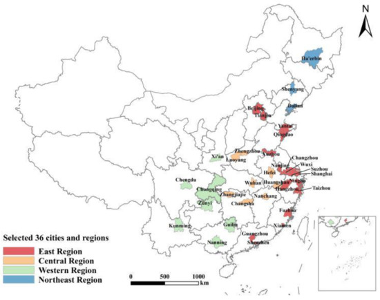
Figure 1.
The 36 selected cities and their regional division.
2.5. Factors That Influence TEE
To further investigate the influence of socioeconomic factors on TEE, the panel data are constructed using STATA 15 for the 36 tourist cities for the 2010 to 2019 period. To mitigate heteroscedasticity, the logarithm for all the original variables is used, resulting in the following regression model [57]:
where i represents 36 tourist cities in China ( = 1, 2, 3..., 11); t represents the year (t = 1, 2, 3..., 10); is the intercept term for each region, i.e., the fixed effect; and is the random error term. denotes the tourism eco-efficiency of municipality in year , measured using the results in the previous section. represents the contribution of tourism to employment in municipality in year , expressed as the ratio of the number of employees in the tourism industry to the number of employees in the tertiary industry, as described in the previous section. To better test the impact of the social and economic development of the 36 tourist cities on TEE, other influencing factors need to be controlled, and the control variable is introduced. The control variables in this study include urbanization (URB), degree of government intervention (GOV), level of economic development (PGDP), and degree of economic openness (OPEN). URB is the ratio of the permanent urban population to the total population, and urbanization drives the labor force to move to tertiary industries and optimizes the industrial structure. GOV is the proportion of local fiscal expenditure in GDP, and it can reasonably allocate resources and compensate for market failure. PGDP is reflected by per capita GDP, and it stimulates consumption and promotes tourism development. OPEN is the amount of foreign capital utilized as a proportion of GDP; foreign enterprises foster technological innovation and organizational management but also cause ecological/environmental pollution.
3. Results
3.1. Analysis of the Eco-Efficiencies of Tourist Cities
3.1.1. Analysis of TEE
As shown in Figure 2, there were significant spatial differences in eco-efficiency among the different cities, and the eco-efficiency of the same city fluctuated across the years. Notably, four cities (Guilin, Huangshan, Sanya, and Zhangjiajie) each had a mean eco-efficiency greater than 1, which is attributed to their relatively high proportion of total tourism revenue to GDP in the absence of additional inputs. In contrast, the eco-efficiencies of Beijing, Guangzhou, Shanghai, Shenzhen, and Chongqing decreased continuously over the years, potentially because these cities were ranked among the top in terms of the number of star-rated hotels, tourist attractions, and travel agencies, as well as carbon emissions and urban wastewater discharge; these excessive “input redundancies” thus directly affected the eco-efficiencies of these cities. From an annual perspective, the mean TEE from 2010 to 2019 was consistently less than 0.5, far from the effective value of 1, indicating that there is still great potential to promote energy conservation and emission reductions, optimize resource allocation, and improve technological capacity. The coefficient of variation (COV) was calculated to further examine the difference in the mean TEE among the different cities from 2010 to 2019. As shown in Figure 2, the COV differs greatly among cities and from year to year, even for cities within the same region. The fundamental reason for this variation is the difference in the resource endowment within each province and the difference in the inputs and outputs of the tourism resources adopted by each province.
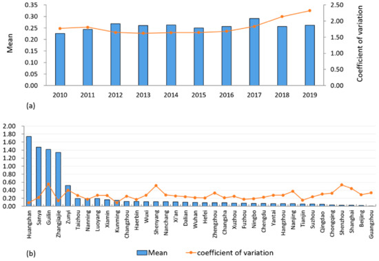
Figure 2.
Changes in the mean and coefficient of variation for the TEE of 36 tourist cities from 2010 to 2019. (a) Temporal changes; (b) spatial changes.
The spatial pattern of the eco-efficiency of the tourist cities is further investigated using 2010, 2013, 2016, and 2019 as the main years of interest. The overall TEE improved temporally (Figure 3). Specifically, the TEE increased continuously from 2010 to 2013 and remained basically unchanged from 2013 to 2016. As economic development entered a new normal in 2017, the growth rate of the tourism economy slowed, affecting the improvement in TEE, resulting in a small decrease in TEE in some cities. Nevertheless, the overall TEE increased with an annual growth rate of 29.53%. For the four major regions, the mean TEE decreased in the following order: central region (0.47), western region (0.36), eastern region (0.15), and northeastern region (0.11). Such low eco-efficiency in these regions indicates substantial waste and inefficient utilization of resources in the tourism products or services.
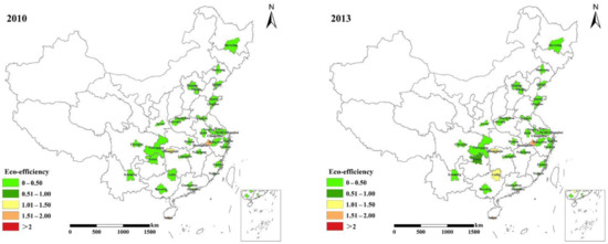
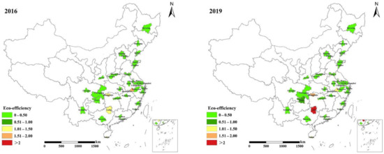
Figure 3.
Spatial distribution of eco-efficiency.
3.1.2. Analysis of TEE by Region
Eco-efficiency was compared across four regions by the decomposed efficiencies, TEC and SEC, to reveal the underlying mechanism of low eco-efficiency (Figure 4). In the ten years from 2010 to 2019, the TEE of the western region increased rapidly, and the other three regions remained stable. The main reason for the formation of this spatiotemporal pattern is that the western region was initially constrained by technological bottlenecks, but its eco-efficiency improved through technological advancement and niche tourism development. Driven by rich tourism resources, the effect of economic scale and industrial structure, the central region maintained higher TEE during the period. Although technological efficiency continuously improved in the eastern region, scale efficiency dropped significantly, resulting in low TEE over the period. The northeastern region had a higher scale efficiency than the eastern region but showed the lowest TEE due to a lack of scientific and technological investment. As shown in Figure 4, the average scale efficiency of 36 cities continued to decrease and reached the lowest level (0.25) in 2019, which is the main reason for the decline in the average TEE.
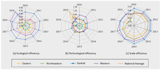
Figure 4.
Changes in regional efficiency.
To understand the correlation among these cities in terms of TEE, spatial autocorrelation was investigated with STATA 13.0, using a geographic distance weight matrix. The test results in Table 2 show that the Moran index is close to 0 and that the values for most years do not pass the significance test (less than 5%), indicating that the TEE of the developed cities was randomly distributed without spatial autocorrelation.
Table 2.
Moran’s index of eco-efficiency from 2010 to 2019.
The eco-efficiency for 2010, 2015, and 2019 was plotted using STATA based on geographical weights. The agglomeration modes of the Moran index of eco-efficiency in 2010, 2015, and 2019 are summarized in Table 3 and are distributed mainly in the second and third quadrants. The results indicate that the eco-efficiency of the tourist cities was dominated by low-low agglomeration, followed by low-high agglomeration, and that the number of cities with high-high agglomeration and high-low agglomeration was the smallest. These results indicate that the low eco-efficiency of the tourist cities was spatially correlated, the low eco-efficiency areas were adjacent to each other, forming agglomerates, and the spatial spillover effect of the high eco-efficiency of the cities was not evident and still has much room for improvement.
Table 3.
Agglomeration modes for the eco-efficiencies of tourist cities.
3.2. Malmquist Model Results
3.2.1. Temporal Changes in the Average Eco-Efficiency of Tourism
Based on the calculation results for the eco-efficiencies of the 36 tourist cities, the Malmquist index (MI) is used to investigate the eco-efficiency trends in the 2010–2019 period. MI > 1 represents an increase in TEE, with a larger MI value indicating a higher increase; conversely, MI < 1 indicates a decrease in TEE. Despite an overall decrease, the MI values for all the cities were greater than 1 (with a mean value of 1.12) over the period, indicating that the overall eco-efficiency of the tourism industry increased from 2010 to 2019 (Figure 5). China was severely impacted by haze and other forms of environmental pollution in the 2013–2014 period, causing eco-efficiency to decrease to its lowest point (1.02), followed by a brief rebound in 2015 after the implementation of relevant energy conservation and emission reduction policies. Due to the new normal during the 2017–2018 period, the tourism economy increased slowly, and eco-efficiency decreased to some extent; late in the period, the TEE rebounded, prompted by the strong policies implemented earlier in the period.
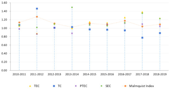
Figure 5.
Malmquist index and its decomposition for tourist cities from 2010 to 2019.
Moreover, the TEC values were greater than 1 for nine years, with an average annual increase of 0.86%; the TC values were greater than 1 only for four years, with an average annual increase of −0.77% (Figure 5). These results indicate that during the study period, the TEC index drove the increase in the MI, and the organizational management and industrial structure of the tourism industry were continuously optimized, but there was a lack of technological development and application of new technologies. From the perspective of the TEC index decomposition, the SEC remained greater than 1, with an average annual increase of 1.04%, while the PTEC values were greater than 1 for seven years, with an average annual increase of 0.46%. These results indicate that the tourist cities did not effectively use the technology that was heavily invested in and could not achieve scale efficiency.
3.2.2. Spatial Evolution of TEE
As shown in Figure 6, the curves for the eastern, northeastern, and central regions are consistent, while the TC value of the western region is significantly greater than that of the other regions, giving the western region the highest Malmquist index. The average annual growth rates of eco-efficiency for the eastern, central, northeastern, and western regions were 2%, 0.82%, 0.48%, and −5.61%, respectively. The advantages in location, economy, transportation, and technological innovation helped the eastern region to improve its eco-efficiency. The northeastern and central regions have much room to improve their technological innovation in the tourism industry. With its rich tourism resources and constantly improving transportation, the western region has a strong latecomer advantage, but the growth rate of ecological efficiency still lags behind that of the other regions. Therefore, cities should implement macro-control measures to maintain steady improvements in eco-efficiency.
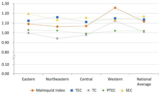
Figure 6.
Spatial difference in eco-efficiency indicators for 2010–2019.
Observed from the perspective of a single city, Nanjing had the highest average annual growth rate of eco-efficiency, 30.12%, with an average growth rate of TC of 32.46% (Figure 7). Guilin obtained an average growth rate of eco-efficiency of −16.22% and an average annual growth rate of TC of −21.13%. This comparison indicates that technological innovation is essential to improving eco-efficiency. In general, 77.7% of the cities had a TEE greater than 1. The average value of TFP for the tourist cities in the 2010–2019 period was 1.12, which can be attributed to the TEC index, indicating that the tourist cities increased their eco-efficiency through improved resource allocation and management capacity and scale effects but lacked technological innovation as well as research and development.
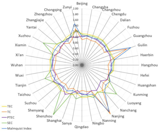
Figure 7.
Malmquist index and its decomposition for tourist cities.
In summary, TEC and PTEC had little impact on total efficiency, of which TC and SEC were more critical. The averages of TEC and SEC were much higher than the average values of TC and PTEC. Therefore, the tourist cities should give top priority to TC, i.e., reform and innovation, and vigorously enhance technological transformation and increase technological investments and scale operations. With rich natural resources, the western region should not only increase technological investments and scale operations but also optimize the organization, management, and structure of the tourism industry and implement macro-control and forecasting to prevent lags in eco-efficiency.
3.3. Cluster Analysis
The above analysis and evaluation using the super-SBM model and the DEA–MI provides the tourism eco-efficiencies of the tourist cities for the 2010–2019 period; overall, the results are not similar among the cities. The k-means cluster analysis was performed using SPSS 25.0 to classify the 36 tourist cities into four categories (Figure 8). As shown in Figure 8, the TEE was not directly related to the degree of economic development and geographic location. For example, both the economically developed Beijing and Shanghai and the economically less developed Harbin and Dalian are classified in the first category, which contains Beijing in the eastern region, Dalian in the northeastern region, Wuhan in the central region, and Chongqing in the western region. The second category contains Guilin, the third category contains Zunyi, and the fourth category contains Zhangjiajie and Huangshan. The overall cluster analysis results show that the tourism eco-efficiencies of the cities in the economically developed and coastal areas are not necessarily the highest. In future development, talent, funds, and relevant policies and regulations should be reasonably allocated to cities based on their resources to improve TEE.
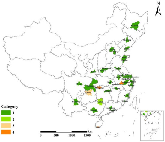
Figure 8.
K-means cluster analysis of the TEE of tourist cities.
3.4. Empirical Results and Analysis
First, to avoid spurious regression, the unit root test for each variable is conducted using the Levin–Lin–Chu (LLC) test in the case of the same roots and the Im–Pesaran–Shin (IPS) test in the case of different roots before conducting panel regression (Table 4). Based on the test results, the null hypothesis, i.e., the “existence of a unit root”, is rejected for the variables URB, GOV, PGDP, and OPEN, and the series is stationary. The significance of TEE is not apparent. However, after the first-order difference, the null hypothesis, i.e., the “existence of a unit root”, is rejected for each variable, and the series is stationary.
Table 4.
Panel unit root tests.
Second, the cointegration test, which presupposes the stationarity of all the variables, is conducted based on the panel unit root tests. Based on the above analysis, the system of variables has a long-term equilibrium relationship (Table 5).
Table 5.
Panel cointegration tests.
In this study, a two-way fixed effect regression model of panel data is used to investigate the impact of the tourism eco-efficiencies of the 36 tourist cities on national economic development. Table 6 provides the regression results after the gradual introduction of the control variables.
Table 6.
Regression coefficient.
As shown in Table 6, the regression coefficients for the core explanatory variable (contribution of tourism to employment) in the model are all positive and are significant at the 5% or 10% significance level, indicating that when controlling for other variables, the rapid development of tourism in the 36 tourist cities played a significant role in promoting TEE. The eco-efficiencies of the tourist cities varied with the influence of factors such as tourism industry structure, TC, urbanization, and intensity of government regulation, but in general, the tourism industry in each region constantly transformed in an eco-efficient direction. Relying on the advantages of history and culture, natural landscapes, and folk customs, each region has developed unique tourism industries by creating tourist cities, boutique routes, tourist attractions, tourist resorts, leisure areas, and ecotourism destinations, and has made efforts to establish an international golden tourism belt.
Regarding the control variables, urbanization was not significantly related to TEE. This result indicates that on the one hand urbanization was accompanied by factor accumulation and industrial structure changes as well as population growth and an increase in carbon emissions, thereby negatively affecting TEE; on the other hand, it promoted the development of social productivity, technological progression, and adjustments to industrial structure, thereby having a positive effect on eco-efficiency. The degree of government intervention was negatively related to eco-efficiency. This is because the amount of government investment is large and the return period is long. As a result, the input increases rapidly in the short term while the output fails to keep up, which leads to the reduction in eco-efficiency. The degree of economic openness and the level of economic development had a positive effect on the eco-efficiencies of the 36 tourist cities because foreign enterprises brought advanced technologies and processes, promoting a reduction in regional resource consumption and environmental pollution. Based on the environmental Kuznets curve (EKC) theory [58], as the level of economic development increases, the industrial structure is upgraded, productivity is influenced by TC, and resource consumption and pollution emissions due to economic development will peak and then decline.
4. Discussion
Food, accommodation, travel, shopping, and entertainment activities are inseparable from carbon emissions and sewage discharges, which place certain pressures on the environment. Examining the tourism efficiency at the cost of undesired outputs is of great significance to the sustainable development of tourism. Based on the data on carbon emissions and urban sewage discharges in 36 tourist cities from 2010 to 2019, the paper evaluated the spatiotemporal characteristics of TEE and its influencing factors using the super-SBM Model, the DEA–Malmquist index, and a two-way fixed effect regression model. Unlike the previous studies, this study quantified the TEE among tourist cities in China to ensure the comparability and representativeness of the data and research conclusions at the national scale. The combination of multiple models and indicators helps to comprehensively explain the TEE change, including the spatiotemporal evolution, the structural dynamics, and the driving factors. In addition, the super-SBM model includes radial and non-radial distance functions to measure eco-efficiency. It makes up for the shortcomings of the traditional radial DEA model and the non-radial SBM model to a certain extent and makes the calculation results of eco-efficiency more real and accurate.
During the study period, the overall eco-efficiency of 36 tourist cities in China in-creased steadily, but the U-shaped Kuznets curve occurred during 2012–2017 [59,60]. Some studies on mainland China also argued for the existence of the Kuznets curve in the process of TEE change [60,61,62,63], but the periods of their appearance were not consistent due to the different scale or variables selected. From 2010 to 2019, the TEE of the 36 tourist cities tended to decline but remained at the relatively higher values, which is related to China’s macroeconomic and national policies. As economic development entered a new normal in 2017, the growth rate of the tourism economy slowed, affecting the TEE improvement. Similarly to the previous research [45,57,58,64], the overall eco-efficiency of the 36 cities selected in this study remained at a low level, which resulted from low scale efficiency.
It is worth noting that the coefficient of variation increased rapidly after 2016, indicating that the eco-efficiency disparity between the cities continued to expand. The central and western regions had higher eco-efficiency than the national average, while the eastern and northeastern regions remained at low eco-efficiency. From high to low, the order of eco-efficiency among the regions was: central region, western region, eastern region, and northeastern region. Recent studies on mainland China, however, argued that the provincial eco-efficiency of tourism was higher in the east than in the middle and the west [45,65,66]. These findings were established at a larger scale and only carbon emission was considered instead of multiple undesired outputs. Moreover, these provinces are not at the same level of tourism development; so, it is not consistent with the conclusions of this paper. The change of TEE reflects the widening eco-efficiency gap among major tourist cities, which will affect the coordinated and sustainable development of the destinations. Therefore, the scientific planning of tourism ecology is essential for destination sustainability, and a refined assessment of tourism efficiency is fundamental for formulating practical policies.
The global correlation test and global autocorrelation test in this paper show that low eco-efficiency areas are predominantly adjacent to each other, while high eco-efficiency areas are occasionally adjacent to low eco-efficiency areas. This conclusion is approximately consistent with the conclusions of Guo [58], but the difference is that the clusters are not globally relevant in our research because the region selected in this study is a decentralized urban agglomeration. Therefore, the cities should actively explore the mechanism of tourism alliances and form a development pattern of regional coordination and industrial interoperability by effectively combining tourism resources and sharing source markets to reduce the gap in the tourism industry between the cities and realize the ideal state of eco-efficient destinations with high-high agglomeration.
Although some scholars have selected cities as research areas [46,64,66], they rarely analyze the dynamic changes and decomposition of tourism eco-efficiency from multiple urban agglomerations. This study has analyzed the specific problems of the eco-efficiency changes in detail. The Malmquist index generally declined, but it was greater than 1 (the average value is 1.12) from 2010 to 2019, indicating that the national tourism industry is in a state of high efficiency and good development. According to Figure 4, the rise in the technological progress index (TC) is the main factor that affects the Malmquist index. This finding is also consistent with the literature [65]. Therefore, those with a low technical progress index should implement technical reform and innovation in the tourism industry. Those with low pure technical efficiency should increase the effectiveness of the input resources, and those whose scale efficiency is less than one should better leverage their economies of scale. In short, the cities should strengthen the quality integration of the tourism practitioners, advocate civilized and healthy tourism, improve infrastructure construction, and vigorously develop smart tourism, health tourism, and eco-tourism to obtain a high quality of tourism development.
Through cluster analysis, it was found that TEE was not directly affected by the location of the cities and the level of economic development but was significantly negatively correlated with urbanization and government intervention, which is consistent with the results of Xia [67]. With the economic growth and urbanization, the environmental pollution increases from low to high, and the degree of environmental degradation increases with economic growth, which is also consistent with the theory of the environmental Kuznets curve (EKC). In addition, tourism eco-efficiency is affected by many factors, which requires us to make full use of the favorable factors and overcome the unfavorable factors. Therefore, the economy should play a leading role in tourism. For example, economically developed cities such as Beijing, Shanghai, and Wuhan can establish ecological compensation mechanisms and implement a range of incentives to encourage innovative green environmental protection projects. For economically underdeveloped areas, such as Zhangjiajie and Taizhou, it is possible to create a niche tourism market, explore new models of tourism development, and promote industrial transformation and upgrading according to local conditions to achieve green growth.
5. Conclusions
With the combined use of the super-SBM model, spatial analysis, the Malmquist index, cluster analysis, and the two-way fixed effect regression model, this paper investigated the spatiotemporal pattern and influencing factors of eco-efficiency among 36 tourist cities and put forward targeted optimization suggestions. Regarding the comparability of the MUDs, 36 developed tourist cities were selected as a representation of the frontier development level of the tourism industry in mainland China. The super-SMB model was used to explore the cross-sectional eco-efficiency of destination cities, while the Malmquist index was used to examine the dynamic pattern of destination eco-efficiency. The spatial correlativity of the cities in terms of eco-efficiency was investigated using the global and local Moran’s index. Based on the performance of tourism eco-efficiency, the selected 36 cities were clustered into four categories to reveal the distribution pattern of tourism eco-efficiency. A regression model was used to explore the mechanism of the tourism eco-efficiency dynamics. The major conclusions obtained are as follows:
The eco-efficiency of the major tourist cities in mainland China continuously increased but was maintained at a low level. The eco-efficiency disparity between the cities tended to increase, reflecting that coordinated development among the tourist cities is facing challenges.
In terms of time, the rise in the overall eco-efficiency of the tourist cities is promoted by the technological efficiency (TEC), and the increment of TEC is contributed mostly by the scale efficiency (SEC). Spatially, the technological progress (TC) is the main driver of the eco-efficiency disparity among tourist cities.
No spatial correlation exists among the eco-efficiencies of the tourist cities, and the eco-efficiency of the economically developed areas is not necessarily higher than that of underdeveloped areas.
To improve ecological efficiency, it is necessary to take a combination of measures, that is, moderately expand the scale of tourism, promote the level of economic development and openness, have control over investment, and improve the utilization of resources.
This paper empirically tests the different effects and related laws of tourism on environmental efficiency, enriches the research content of the tourism resources and the environmental economy to a certain extent, promotes the integration of tourism geography, the spatial economy, and the ecology, and provides a scientific reference point for the sustainable development and common development of tourism to a certain extent. The problem of tourism ecology is the result of many factors and the embodiment of the law of economic and social development. To realize the coordinated and sustainable development of tourism and the ecological environment, we should not only recognize the reality of the development stage of tourism but also respect the principle of environmental protection.
Admittedly, due to objective conditions with respect to the data and methods used in the research process, this study has the following limitations. First, the spatial weight matrix used in this study considers spatial distance only. Although this method is easy to use, it does not consider factors such as economic distance, which may lead to conservative and biased estimates. Second, constrained by data availability, only 36 tourism cities were selected as the research objects in this study. In the future, we can, for example, choose a wider range of cities and representative regions or reflect more on the relationship between tourism and the environment. Finally, the factors that influence eco-efficiency are not limited to the economic factors addressed in this study but include other factors that affect environmental efficiency, such as environmental regulations and resource competition. In the future, we can establish a complete environmental efficiency system. Exploring the theoretical mechanisms and conducting empirical tests of factors that affect eco-efficiency are important future research directions.
Author Contributions
Conceptualization, P.M.; methodology, C.A.; software, C.A.; validation, P.M.; formal analysis, C.A.; data curation, C.A. and Z.X.; writing—original draft preparation, C.A; writing—review and editing, P.M.; visualization, Z.X.; supervision, P.M.; project administration, P.M.; and funding acquisition, P.M. All authors have read and agreed to the published version of the manuscript.
Funding
This research was funded by the National Natural Science Foundation of China, grant numbers 41961038 and 41661106, and the Key Laboratory Projection of Sustainable Development of Xinjiang’s Historical and Cultural Tourism, Xinjiang University, grant number LY2022-04.
Data Availability Statement
Tourism-related statistics can be obtained from the China Economic and Social Big Data Research Platform (https://data.cnki.net/yearbook (accessed on 16 September 2021)). The data presented in this study are available on request from the corresponding author.
Acknowledgments
We acknowledge all the data sources for this paper. We are also grateful to the editor and the reviewers for their helpful comments.
Conflicts of Interest
The authors declare no conflict of interest.
References
- Lenzen, M.; Sun, Y.Y.; Faturay, F.; Ting, Y.P.; Geschke, A.; Malik, A. The carbon footprint of global tourism. Nat. Clim. Chang. 2018, 8, 522–528. [Google Scholar] [CrossRef]
- Tang, Z.; Shang, J.; Shi, C.; Liu, Z.; Bi, K. Decoupling indicators of CO2 emissions from the tourism industry in China: 1990–2012. Ecol. Indic. 2014, 46, 390–397. [Google Scholar] [CrossRef]
- Zhang, J.; Zhang, Y. Carbon tax, tourism CO2 emissions and economic welfare. Ann. Tour. Res. 2018, 69, 18–30. [Google Scholar] [CrossRef]
- Lee, L.C.; Wang, Y.; Zuo, J. The nexus of water-energy-food in China’s tourism industry. Resour. Conserv. Recycl. 2021, 164, 105157. [Google Scholar] [CrossRef] [PubMed]
- Chenghu, Z.; Arif, M.; Shehzad, K.; Ahmad, M.; Oláh, J. Modeling the Dynamic Linkage between Tourism Development, Technological Innovation, Urbanization and Environmental Quality: Provincial Data Analysis of China. Int. J. Environ. Res. 2021, 18, 8456. [Google Scholar] [CrossRef]
- Chen, Q.; Mao, Y.; Morrison, A.M. Impacts of Environmental Regulations on Tourism Carbon Emissions. Int. J. Environ. Res. Public Health 2021, 18, 12850. [Google Scholar] [CrossRef]
- Mikayilov, J.I.; Mukhtarov, S.; Mammadov, J.; Azizov, M. Re-evaluating the environmental impacts of tourism: Does EKC exist? Environ. Sci. Pollut. Res. Int. 2019, 26, 19389–19402. [Google Scholar] [CrossRef]
- Calderwood, L.U.; Soshkin, M. The Travel & Tourism Competitiveness Report 2019. World Economic Forum, Geneva. 2019, p. 31. Available online: https://www3.weforum.org/docs/WEF_TTCR_2019.pdf (accessed on 8 September 2022).
- Song, M.; Li, H. Estimating the efficiency of a sustainable Chinese tourism industry using bootstrap technology rectification. Technol. Forecast. Soc. 2019, 143, 45–54. [Google Scholar] [CrossRef]
- Shi, Y.; Yu, M. Assessing the Environmental Impact and Cost of the Tourism-Induced CO2, NOx, SOx Emission in China. Sustainability 2021, 13, 604. [Google Scholar] [CrossRef]
- Yu, Y.; Chen, D.; Zhu, B.; Hu, S. Eco-efficiency trends in china, 1978–2010: Decoupling environmental pressure from economic growth. Ecol. Indic. 2013, 24, 177–184. [Google Scholar] [CrossRef]
- Gössling, S.; Peeters, P.; Ceron, J.; Dubois, G.; Patterson, T.; Richardson, R.B. The eco-effificiency of tourism. Ecol. Econ. 2005, 54, 417–434. [Google Scholar] [CrossRef]
- Liu, J.; Ma, Y. The perspective of tourism sustainable development: A review of eco-effificiency of tourism. Tour. Trib. 2017, 32, 47–56. (In Chinese) [Google Scholar]
- Becken, S.; Frampton, C.; Simmons, D.G. Energy consumption patterns in the accommodation sector: The New Zealand case. Ecol. Econ. 2001, 39, 371–386. [Google Scholar] [CrossRef]
- Becken, S.; Patterson, M. Measuring national carbon dioxide emissions from tourism as a key step towards achieving sustainable tourism. J. Sustain. Tour. 2006, 14, 323–338. [Google Scholar] [CrossRef]
- Assaf, A.G.; Josiassen, A. Frontier analysis: A state-of-the-art review and meta- analysis. J. Travel Res. 2016, 55, 612–627. [Google Scholar] [CrossRef]
- Qiu, X.; Fang, Y.; Yang, X.; Zhu, F. Tourism eco-efficiency measurement, characteristics, and its influence factors in China. Sustainability 2017, 9, 1634. [Google Scholar] [CrossRef]
- Emrouznejad, A.; Yang, G.L. A survey and analysis of the first 40 years of scholarly literature in DEA: 1978–2016. Soc. Econ. Plann. Sci. 2018, 61, 4–8. [Google Scholar] [CrossRef]
- Altin, M.; Koseoglu, M.A.; Yu, X.; Riasi, A. Performance measurement and management research in the hospitality and tourism industry. Int. J. Contemp. Hosp. Manag. 2018, 30, 1172–1189. [Google Scholar] [CrossRef]
- Perch-Nielsen, S.; Sesartic, A.; Stucki, M. The greenhouse gas intensity of the tourism sector: The case of Switzerland. Environ. Sci. Policy 2010, 13, 131–140. [Google Scholar] [CrossRef]
- Farrell, M.J. The measurement of productive efficiency. J. R. Stat. Soc. 1957, 120, 253–290. [Google Scholar] [CrossRef]
- Charnes, A.; Cooper, W.W.; Rhodes, E. Measuring the efficiency of decision-making units. Eur. J. Oper. Res. 1978, 2, 429–444. [Google Scholar] [CrossRef]
- Ramanathan, R. An Introduction to Data Envelopment Analysis: A Tool for Performance Measurement; Sage: London, UK, 2003. [Google Scholar]
- Sexton, T.R.; Silkman, R.H.; Hogan, A.J. Data envelopment analysis: Critique and extensions. New Dir. Program Eval. 1986, 1986, 73–105. [Google Scholar] [CrossRef]
- Mantri, J.K. Research Methodology on Data Envelopment Analysis (DEA); Universal-Publishers: Irvine, CA, USA, 2008. [Google Scholar]
- Ruan, W.; Li, Y.; Zhang, S.; Liu, C. Evaluation and drive mechanism of tourism ecological security based on the DPSIR-DEA model. Tour. Manag. 2019, 75, 609–625. [Google Scholar] [CrossRef]
- Walz, A.; Calonder, G.P.; Hagedorn, F. Regional CO2 budget, countermeasures and reduction aims for the Alpine tourist region of Davos, Switzerland. Energy Policy 2008, 36, 811–820. [Google Scholar] [CrossRef]
- Peter, T. Climate Change Mitigation: Methods, Greenhouse Gas Reductions and Policies; NHTV: Breda, The Netherlands, 2007. [Google Scholar]
- Susanne, B. Developing indicators for managing tourism in the face of peak oil. Tour. Manag. 2008, 29, 695–705. [Google Scholar]
- Gossling, S. Carbon Management in Tourism: Mitigating the Impacts on Climate Change; Routledge: London, UK, 2010. [Google Scholar]
- Janet, E.; Dickinson, D.R.; Les, L. Holiday travel discourses and climate change. J. Transp. Geogr. 2010, 18, 482–489. [Google Scholar]
- Aigner, D.; Lovell, C.A.K.; Schmidt, P. Formulation, and estimation of stochastic frontier production function models. J. Econom. 1977, 6, 21–37. [Google Scholar] [CrossRef]
- Meeusen, W.; Van, D.; Broeck, J. Efficiency estimation from Cobb-douglas production functions with composed error. Int. Econ. Rev. 1977, 18, 435–444. [Google Scholar] [CrossRef]
- Reifschneider, D.; Stevenson, R. Systematic departures from the frontier: A framework for the analysis of firm inefficiency. Int. Econ. Rev. 1991, 32, 715–723. [Google Scholar] [CrossRef]
- Kumbhakar, S.C.; Ghosh, S.; McGuckin, J.T. A generalized production frontier approach for estimating determinants of inefficiency in U.S. dairy farms. J. Bus. Econ. Stat. 1991, 9, 279–286. [Google Scholar]
- Battese, G.E.; Coelli, T.J. Frontier production functions, technical efficiency, and panel data: With application to paddy farmers in India. J. Prod. Anal. 1992, 3, 153–169. [Google Scholar] [CrossRef]
- Battese, G.E.; Coelli, T.J. A model for technical inefficiency effects in a stochastic frontier production function for panel data. Empir. Econ. 1995, 20, 325–332. [Google Scholar] [CrossRef]
- Zhao, P.J.; Zeng, L.G.; Li, P.L.; Lu, H.Y.; Hu, H.Y.; Li, C.M.; Zheng, M.Y.; Li, H.T.; Yu, Z.Y.; Yuan, D.; et al. China’s transportation sector carbon dioxide emissions efficiency and its influencing factors based on the EBM DEA model with undesirable outputs and spatial Durbin model. Nat. Energy 2022, 238, 121934. [Google Scholar] [CrossRef]
- Pedolin, D.; Six, J.; Nemecek, T. Assessing between and within Product Group Variance of Environmental Efficiency of Swiss Agriculture Using Life Cycle Assessment and Data Envelopment Analysis. Agron. J. 2021, 11, 1862. [Google Scholar] [CrossRef]
- Çağlar, O.D. The Turkish Cypriot Municipalities’ Productivity and Performance: An Application of Data Envelopment Analysis and the Tobit Model. J. Risk Financ. Manag. 2021, 14, 407. [Google Scholar] [CrossRef]
- Zhou, W.Z.; Yu, W.H.; Farouk, A. Regional Variation in the Carbon Dioxide Emission Efficiency of Construction Industry in China: Based on the Three-Stage DEA Model. Discret. Dyn. Nat. Soc. 2021, 2021, 4021947. [Google Scholar] [CrossRef]
- Andersen, P.; Petersen, N.C. A Procedure for Ranking Efficient Units in Data Envelopment Analysis. Manag. Sci. 1993, 39, 1261–1264. [Google Scholar] [CrossRef]
- Pan, Y.; Weng, G.; Li, C. Coupling Coordination and Influencing Factors among Tourism Carbon Emission, Tourism Economic and Tourism Innovation. Int. J. Environ. Res. Public Health 2021, 18, 1601. [Google Scholar] [CrossRef]
- Tone, K. A slacks-based measure of efficiency in data envelopment analysis. Eur. J. Oper Res. 2001, 130, 498–509. [Google Scholar] [CrossRef]
- Wang, R.; Xia, D.S.; Li, Y.; Li, Z.; Ba, D.; Zhang, W.B. Research on the Spatial Differentiation and Driving Forces of Eco-Efficiency of Regional Tourism in China. Sustainability 2020, 13, 280. [Google Scholar] [CrossRef]
- Sun, Y.; Hou, G.; Huang, Z.; Zhong, Y. Spatial-Temporal Differences and Influencing Factors of Tourism Eco-Efficiency in China’s Three Major Urban Agglomerations Based on the Super-EBM Model. Sustainability 2020, 12, 4156. [Google Scholar] [CrossRef]
- Li, B.; Ma, X.; Chen, K. Eco-efficiency measurement and spatial–temporal evolution of forest tourism. Arab. J. Geosci. 2021, 14, 568. [Google Scholar] [CrossRef]
- Castilho, D.; Fuinhas, J.A.; Marques, A.C. The impacts of the tourism sector on the Eco-efficiency of the Latin American and Caribbean countries. Socio-Econ. Plan. Sci. 2021, 78, 101089. [Google Scholar] [CrossRef]
- Yu, W.; Chen, T.; Yu, S.; Wang, H. Study on spatial-temporal distribution and dynamic evolution of Eco-efficiency in China’s coastal provinces. J. Coast. Res. 2020, 106, 454. [Google Scholar] [CrossRef]
- Li, Y.; Zhang, L. Ecological effificiency management of tourism scenic spots based on carbon footprint analysis. Int. J. Low-Carbon Technol. 2020, 15, 550–554. [Google Scholar] [CrossRef]
- Peng, H.; Zhang, J.; Lu, L.; Tang, G.; Yan, B.; Xiao, X.; Han, Y. Eco-effificiency and its determinants at a tourism destination: A case study of Huangshan National Park, Tour. Manag. 2017, 60, 201–211. [Google Scholar]
- Hu, M.J.; Ding, Z.S.; Li, Z.J.; Zhou, N.X.; Li, X.; Zhang, C. Ecological Welfare and driving factors of tourism in the perspective of ecological efficiency—A case study of Changzhou City. Acta Ecol. Sin. 2020, 40, 1944–1955. (In Chinese) [Google Scholar]
- Wang, S.; Hu, Y.; He, H.; Wang, G. Progress, and prospects for tourism footprint research. Sustainability 2017, 9, 1847. [Google Scholar] [CrossRef]
- Färe, R.; Grosskopf, S.; Lindgren, B. Productivity changes in Swedish pharamacies 1980-1989: A non-para-metric Malmquist approach. J. Prod. Anal. 1992, 3, 85–101. [Google Scholar] [CrossRef]
- Nurmatov, R.; Fernandez, L.X.L.; Coto, M.P.P. Tourism, hospitality, and DEA: Where do we come from and where do we go? Int. J. Hosp. Manag. 2021, 95, 102883. [Google Scholar] [CrossRef]
- Sten, M. Index numbers and indifference surfaces. Trab. Estad. 1953, 4, 202–242. [Google Scholar]
- Capacci, S.; Scorcu, A.E.; Vici, L. Seaside tourism and eco-labels: The economic impact of Blue Flags. Tour. Manag. 2015, 47, 88–96. [Google Scholar] [CrossRef]
- Guo, L.J.; Li, C.; Peng, H.S.; Zhong, S.E.; Zhang, J.H.; Yu, H. Evaluation and spatial pattern of China’s provincial tourism ecological efficiency under the constraints of energy conservation and emission reduction. Prog. Geogr. Sci. 2021, 40, 1284–1297. (In Chinese) [Google Scholar] [CrossRef]
- Papavasileiou, E.F.; Tzouvanas, P. Tourism Carbon Kuznets-Curve Hypothesis: A Systematic Literature Review and a Paradigm Shift to a Corporation-Performance Perspective. J. Travel Res. 2021, 60, 896–911. [Google Scholar] [CrossRef]
- Ayamba, E.C.; Haibo, C.; Ke, D.; Fangfang, W. The spatial effect of tourism economic development on regional ecological efficiency. Environ. Sci. Pollut. Res. 2021, 27, 38241–38258. [Google Scholar]
- Zaman, K.; Shahbaz, M.; Loganathan, N.; Raza, S.A. Tourism development, energy consumption and Environmental Kuznets Curve: Trivariate analysis in the panel of developed and developing countries. Tour. Manag. 2016, 54, 275–283. [Google Scholar] [CrossRef]
- Xue, D.; Yue, L.; Ahmad, F.; Draz, M.U.; Chandio, A.A. Urban eco-efficiency and its influencing factors in Western China: Fresh evidence from Chinese cities based on the US-SBM. Ecol. Indic. 2021, 127, 107784. [Google Scholar] [CrossRef]
- Xia, B.; Dong, S.; Li, Z.; Zhao, M.; Sun, D.; Zhang, W.; Li, Y. Eco-Efficiency and Its Drivers in Tourism Sectors with Respect to Carbon Emissions from the Supply Chain: An Integrated EEIO and DEA Approach. Int. J. Environ. Res. Public Health 2022, 19, 6951. [Google Scholar] [CrossRef] [PubMed]
- Sun, Y.; Hou, G. Analysis on the Spatial-Temporal Evolution Characteristics and Spatial Network Structure of Tourism Eco-Efficiency in the Yangtze River Delta Urban Agglomeration. Int. J. Environ. Res. Public Health 2021, 5, 2577. [Google Scholar] [CrossRef]
- Zha, J.; Yuan, W.; Dai, J.; Tan, T.; He, L. Eco-efficiency, eco-productivity and tourism growth in china: A non-convex metafrontier DEA-based decomposition model. J. Sustain. Tour. 2020, 28, 663–685. [Google Scholar] [CrossRef]
- Yang, Y.Z.; Yan, J.X.; Yang, Y.; Yang, Y. Spatial and Temporal Evolution and Spatial Spillover Effect of Tourism Ecological Efficiency in the Yellow River Valley-Analysis Based on 73 City Data. Acta Ecol. Sin. 2022, 20, 1–11. (In Chinese) [Google Scholar]
- Xiia, S.S.; Guo, S.F. Ecological Efficiency in the Yellow River Basin: Spatial-Temporal Characteristics and Influencing Factors-Based on the Panel Data of 51 Prefecture-level Cities. J. Stat. 2021, 2, 43–57. (In Chinese) [Google Scholar]


Publisher’s Note: MDPI stays neutral with regard to jurisdictional claims in published maps and institutional affiliations. |
© 2022 by the authors. Licensee MDPI, Basel, Switzerland. This article is an open access article distributed under the terms and conditions of the Creative Commons Attribution (CC BY) license (https://creativecommons.org/licenses/by/4.0/).