Design and Employing of a Non-Linear Response Surface Model to Predict the Microbial Loads in Anaerobic Digestion of Cow Manure: Batch Balloon Digester

Abstract

Biogas is among the sources of renewable energy with a great potential to mitigate global energy challenges by virtue of the ease of implementation of the technology. The study focused on monitoring the total viable bacteria counts with the number of days, daily average ambient temperature and pH from a balloon type biodigester fed with 2500 L of cow manure (500 L of slurry each day for five successive days) with six months retention time using data acquisition system, standard methods and mathematical model. A non-linear response surface model was developed to predict the total viable bacteria counts with the predictors. The predictors were ranked by weights of importance to the desired targets by reliefF test. At the end of the anaerobic digestion cycle the cumulative volume of biogas was 6.75 m³ with 65.8% methane and 31.2% carbon dioxide. The ranking by weights of the predictors revealed that all the input parameters were primary factors and number of days contributed the most. Based on the testing data set, the response surface model was capable of predicting the total viable bacteria counts with high accuracy as the determination coefficient, root mean square error and p-value were 0.959, 0.197 and 0.602.

1. Introduction

An efficient balance of meeting the rising energy demand and limiting its environmental consequences is a cause for concern in the 21st century [1]. Governments in different countries without the exemption of South Africa, have been exploring strategies in developing regulations and policies to encourage eco-friendly renewable energy generation in conjunction with conservation measures and technological innovations. It is of paramount importance to mention that as part of the mitigated challenges in the domain of energy production and environmental impact, South Africa has embarked on the utilization of biogas plants to produce biogas as one of the sources of renewable energy. The study focused on the designed and deployment of a data acquisition system to monitor the potential biogas yield and to develop a response surface model to predict the total bacteria counts in a balloon digester fed with cow waste.

A review on the world biogas generation over the past 10 years shows an increase of almost 90% in biogas industry with a figure of 120 GW in 2019 as opposed to 65 GW in 2010 [2]. The authors proved that in 2017, Europe contributed to 70% of the world biogas generation with an energy consumption of 64 TWh. The conclusion from the review revealed that Europe has the highest promotion rate of biogas generation, whereas the maximum consumption rate is recorded in India and China due to their up-to-date policies and procedures. Research on the review of installation of biogas plants and its generated electricity in Africa, shows that the South Africa has the largest share of the installed biogas plants (approximately 700 plants) and only 300 of the plants has been in operation since 2007 [3]. The study predict that the installed biogas plants have the potential of generating 148 GWh electricity through appropriate investment and implementation schemes.

The practices of livestock are associated with enormous amount of animal manure and call for efficient management to avoid adverse health impact and environmental degradation. The implementation of standard best practices in the efficient disposal and effective management of these animal waste provides potential remedies to eradicate pollutions from the emission of greenhouse gases and reduction in diseases based on water and soil contamination [4]. Enormous research has confirmed that the utilization of anaerobic digesters can serve as an efficient tool of proper management of animal manure. The anaerobic digestion occurring in biodigesters results in the generation of biogas and digestate [5]. The generated biogas from anaerobic fermentation is a renewable source of energy with a wide application such as heating, cooking, transportation and electricity and contribute to the efficient management of animal waste resulting in tremendous decreased in microbial loads [6]. Digestion of dairy cow manure by the method of anaerobic digestion involved the decomposition of organic matter embedded in the livestock substrate by the interaction of four distinct metabolically connected microbes under the hydraulic, acidogenic, acetogenic and methanogenic phases to produce methane, carbon dioxide and other trace gases [7]. Organic waste substrates composed of adequate quantities of nutrients required for the growth and metabolism of the anaerobic bacteria responsible for the generation of biogas [8]. In the Fort Hare dairy farm located in the Eastern Cape province in South Africa, the animal waste is mixed with water and discarded into a lagoon nearby, which is considered to be a storage and treatment plant. The lagoon is not confined, and the stored manure undergoes fermentation emitting carbon dioxide and methane into the atmosphere. Carbon dioxide and methane are greenhouse gases that strongly contribute to climate change and global warming potential [9]. The installation and utilization of anaerobic biodigesters on the Fort Hare cow dairy farm can serve as a clean technology capable of generating renewable energy from the produced biogas while rendering an alternative option of waste management [10]. Despite the exploration of animal manure in the production of biogas through anaerobic digestion (mono-digestion and co-digestion), biogas potential and quality differ with the chemical composition, microbial and biological availability of the nutrients in the animal waste [11]. Furthermore, ambient weather condition and soil characteristics can impact the physicochemical attributes of the animal waste, the species of the animal, dietary sources, state of health of the animals, age of animals and factors affecting the growth of the animals [12].

In this study, we focused on the biogas yield potential of dairy manure collected from the Fort Hare Farm, Eastern Cape province of South Africa by monitoring the physicochemical parameters and microbial loads of the digesting substrate in an anaerobic digestion in a balloon biodigester operating in a single phase, batch mode under mesophilic temperature range. More so, a non-linear response surface model was developed to establish the correlation between the log of total bacterial counts and the input parameters (number of days, daily slurry temperature and pH). The prediction of the desired output was simulated with each input parameter, whereas the rest were held constant using a 2D multi-contour surface plots method [13]. In addition, the reliefF test was used to rank the input parameters according to the weights of importance to the log of the total bacteria counts.

The novelty of the study is the employment of a statistical test known as the reliefF to rank the selected input parameters (number of days, daily slurry temperature and pH) according to the weights of importance of the output parameter (total bacteria counts) and the utilization of a developed response surface model in establishing a simulation that comprised 2D multi-contour surface plots to show the variation in the total bacteria counts with each input parameter, whereas the others are held constant.

1.1. Common Types of Available Biodigesters

The primary design of an anaerobic digestion system is predominantly governed by technical reliability, efficient cost, and the availability of local skills and materials [14]. The common types of biodigesters implemented for anaerobic digestion are the fixed-dome digester, the floating-drum digester and the balloon digester. The bulk of these digesters are wet digestion systems, which operate in either batch or continuous mode under mesophilic conditions.

1.1.1. Fixed-Dome Biodigester

A fixed-dome plant is composed of a closed dome shape digester with an immobile, rigid gas-holder, an influent intake tank, and an effluent outlet tank, as shown in Figure 1. The biogas generated in the biodigester is stored in the upper part of the reactor. The increase in gas production result in an elevation of the interior pressure of the biodigester and assist in displacing the digestate into the outlet tank. A typical fixed-dome biodigester is constructed underground to avoid fluctuation of slurry temperature and maintaining apparent constant temperature during the hydraulic retention time of the anaerobic digestion process. The variability of gas pressure in a fixed-dome biodigester subjects the system to potential biogas leaks and make the utilization not user friendly [15]. The major advantages of fixed-dome biodigester ranged from low cost of construction, long lifespan, no movable parts, no corrosive parts, minimal fluctuation in slurry temperature and the creation of job opportunities for skilled local technicians [16].

1.1.2. Floating-Drum Digester

A floating-drum biogas plant comprised a cylindrical digester and a movable floating drum as shown in Figure 2. The digester is commonly constructed underground whereas the floating drum is above the ground. The digested section of the reactor is frequently constructed with bricks, concrete, or quarry stone masonry, and then plastered [17]. The floating drum is often designed from metal and coated with oil paints to protect the drum against corrosion. A properly maintained floating drum can last for 3–5 years in humid weather conditions and between 8 and 12 years in dry climate [18]. In addition, braces are positioned on the inside of the floating drum, which aid in breaking the scum layer when the drum is rotated. A guiding structure may be implanted inside the gas drum as an extra measure to reduce the degree of tilting of the drum as it rises due to biogas generation. The produced gas collected in the gas drum can either rise or fall based on the volume of biogas produced and utilized. The major advantages of the floating drum digesters are simplicity in construction, relative constant pressure, visibility in the volume of gas stored, and the operation and maintenance procedure are relatively simple.

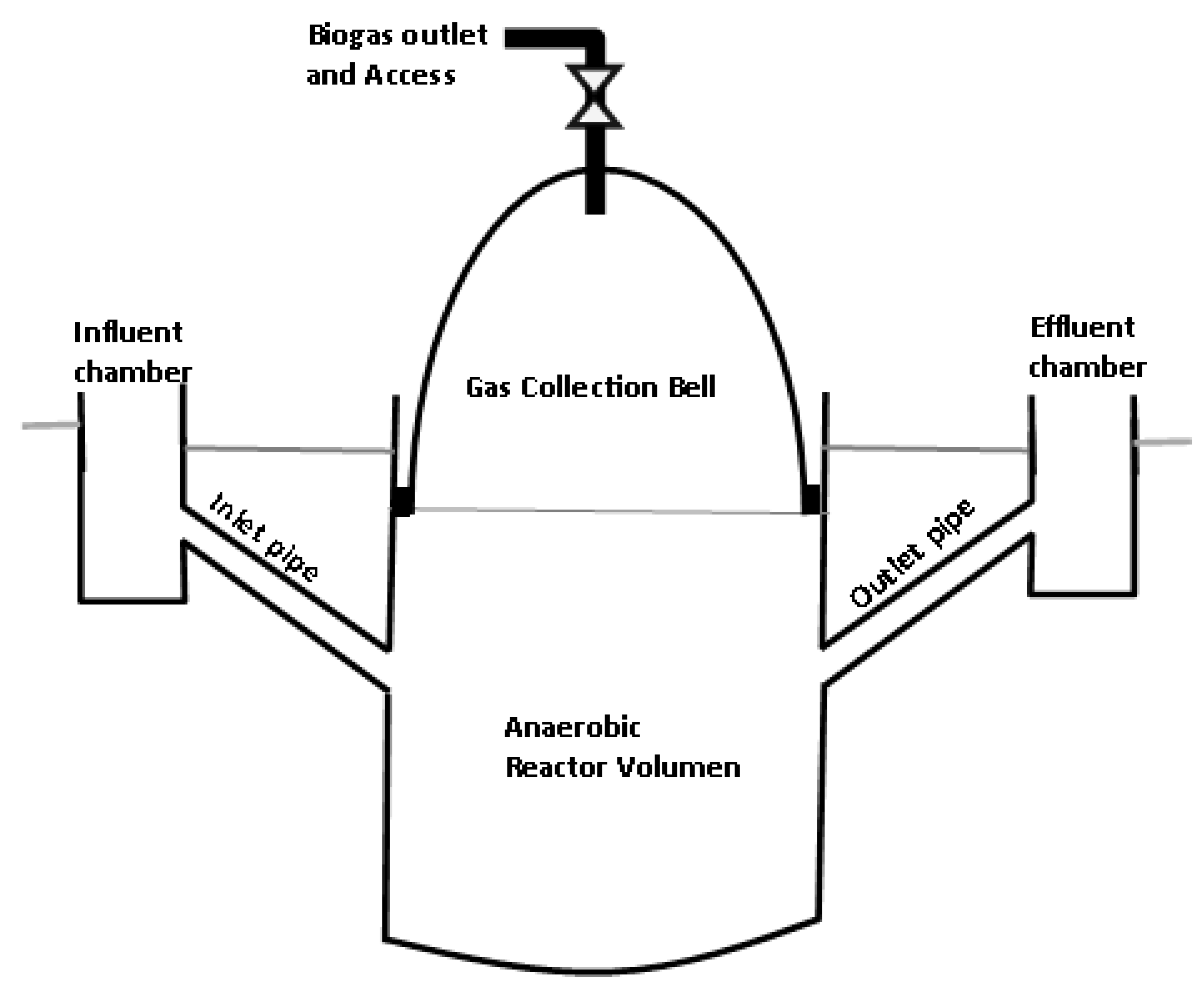
1.1.3. Balloon Digester

A balloon biogas plant constitutes of a longitudinal heat-sealed and weather resistance plastic bag that acts as digester and gas holder in a single compartment as presented in Figure 3 (Schematic diagram of the experimental setup of the study). The gas is stored in the upper part of the balloon, whereas the inlet and outlet are attached directly to the body of the balloon. The no-stirring element is incorporated in balloon digesters, and active mixing is limited, whereas the digestate flows through the reactor in a plug-flow manner. Gas pressure may be increased by introducing weights on the balloon but ensuring that no damage occurs in the process. Additionally, the installation is often at a shallow depth underground, making the system suitable in areas with a high groundwater table. The plastic balloon is quite fragile and prom to mechanical damage and has a relatively short lifespan of 2–5 years [19]. The advantages of balloon digester involved low costs of construction, portability capability and limited challenges as far as transportation is concerned, very high slurry temperature under prevailing warm climatic condition, negligible complexity with respect to operation and maintenance and a shallow installation depth encouraging the utilization of the technology in areas with high ground water table and hard bedrock.

1.2. Factors Contributing to the Yield of Biogas in a Biodigester

1.2.1. Carbon/Nitrogen (C/N) Ratio

The quantity of carbon and nitrogen available in organic matter can be represented by the carbon/nitrogen (C/N) ratio. The efficient and proper degradation of organic material by microorganism is associated with a suitable C/N ratio available in the substrate [20]. Researchers have confirmed that during digestion, microorganisms are capable of utilizing carbon in the range of 25–30 times more than nitrogen [21,22]. Therefore, suitable feedstock for an anaerobic digestion should have a C/N ratio in the order of 25:1 to 30:1 with the percentage of dry matter between 7 and 10%. Despite this, the specified optimal specifications for the C/N ratio and the concentration of dry matter, the waste substrate, can only undergo efficient anaerobic digestion provided the feedstock is biodegradable [23].

1.2.2. Slurry Temperature

The majority of installed biodigesters deployed to the field are not embedded with temperature control mechanism and tool capable to remove dissolved oxygen. The performance of digesters is adversely impacted under low temperature and during the winter period. The different temperature regimes during anaerobic digestion include psychrophilic (<20 °C), mesophilic (20 °C < slurry temperature < 30 °C) and thermophilic (40 °C < slurry temperature < 60 °C) regimes. The mesophilic and thermophilic digestion is influenced by climatic weather conditions in which the plants are subjected therein. Furthermore, thermophilic fermentation can be initiated with external heat source, but the process is inefficient. Moreover, the duration of the fermentation process is strongly correlated to the slurry temperature of the digester with the optimum temperature around 35 °C [24]. On the contrary, when ambient temperature was below 10 °C, the production of biogas in a digester virtually ceased. A stable and favourable production of biogas occurred in the mesophilic range. A robust insulation of digester can assist in increasing the biogas yield under cold weather conditions [25]. It can be stipulated that when a digester operates at 15 °C, it takes almost a year for the digestion process to be completed, but when operated at 35 °C, it may take less than a month [26]. Basumatary et al. [27] conducted experiments on the analysis of the effect of temperature variation on anaerobic digestion of cattle waste. Mahmudul et al. [28] articulated in their research paper that at cold weather condition, biogas plant with reliable design modifications can operate properly as in a warm climate but the complexity and cost of manufacturing such system is limiting the uptake of the proposed designed digester.

1.2.3. pH Value

It is of paramount importance to measure the pH of any feedstock before charging a digester. A pH scale can range from neutral (7) to acidic (1 < pH < 7) or alkaline (7 < pH < 14). The anaerobic digestion process is efficient when the medium of the microorganism is neutral or slightly alkaline [29]. An optimum biogas yield is attained when the pH value of the intake substrate in the digester ranged from 6.25 to 7.50 [30]. The pH value in a biogas digester depends on the retention time. In the early phase of fermentation, the huge level of organic acids produced by acid forming bacteria is forced to decrease the pH value inside the digester to less than 5. This inhibits the digestion process. Methanogenic bacteria are reactive to such pH value and fail to thrive at pH value below 6.5. Later, as the digestion progresses, the concentration of NH4 increases due to the digestion of nitrogen (N2), which lead to an increase in the pH value to above 8. As the methane (CH4) production level attained stability, the pH value ranged from 7.2 to 8.2. Studies have revealed that anaerobic digestion in a digester takes about 6 days for the pH value to become stable when the ambient temperature is fluctuating between 22 and 26 °C [31]. The variation of the ambient temperature between 18 and 20 °C, can force the pH to become stable in approximately 14 to 18 days [32].

1.2.4. Dilution and Consistency of Input

All waste materials required to feed biogas plant consist of solid substance, volatile organic matter, non-volatile matter (fixed solids) and water. During anaerobic digestion process, volatile solids are digested, and non-volatile solids remain unaffected. The finding from Yadav et al. [33] confirmed that fresh cattle waste consists of approximately 20% total solid (TS) and 80% water. TS, in turn, consists of 70% volatile solids and 30% fixed solid. For optimum gas production through anaerobic digestion, 8–10% TS is needed to feed the digester, as confirmed by Yadav et al. [33]. This is achieved by mixing the slurry of fresh cattle manure in water in the ratio of 1:1. However, if the dung is in dry form, the quantity of water needs to increase to meet the desired consistency of the input (maybe the ratio could vary from 1:1.25 to 1:2). It is best practice to remove inert materials such as stones from the inlet chamber before feeding the slurry into the digester.

1.2.5. Loading Rate

Loading rate is referred to the quantity of raw materials fed per day per unit volume of digester capacity. The loading rate affects biogas yield as over-feeding of the digester will result in accumulation of acids and methane production and the yield will be inhibited. This is because the microorganism cannot thrive in acidic situation. On the other hand, under-feeding will reduced the biogas production as result of the creation of an alkaline medium, which is not favourable for anaerobic bacteria [34]. Researchers have proved that a 50 kg charge on daily basis and 100 kg charge on an alternate daily basis produced 2.9043 and 2.9285 m³ of biogas, respectively. However, for a particular size of plant, there is an optimum feed of charge rate that can produce optimum levels of biogas and exceed the quantity of charge, which can lead to a reduction in the biogas production [35]. According to Sreekrishnan et al. [36], the daily loading rate of 16 kg of volatile solids per m³ of digester capacity can yield 0.04–0.074 m³ of biogas per kg of raw dung fed. The authors recommended the loading rates for plants working on night soil to range from 1.04 to 2.23 kg of volatile solids per m³ of digester capacity. Higher loading rates are recommended only in cases where mean ambient temperature is high. Gunaseelan [37] developed a mathematical model to describe biogas yield as a function of organic loading rate and on two different digester designs (continuously stirred tank and non-mixed vertical flow reactor). Analysis of the operation of digesters with the aid of mathematical model suggest that optimum biogas yield could be achieved by selecting a digester design and an operating technique that will increase solid conversion through longer solids and microorganism retention.

1.2.6. Hydraulic Retention Time

Hydraulic retention time (HRT) is the average duration that a specific quantity of feedstock substrate remains in the digester and is acted upon by the methanogens. In a cattle-manure biodigester, the retention time is derived by determining the total volume of the digester by daily volume intake substrate. Ihara et al. [38] postulated that HRT is a function of the inside temperature of the digester and a higher temperature of the digester insinuates lower retention time. HRT usually ranges from 20 to 120 days and is influenced by the design and working temperature of the digester. The digester operating in tropical countries typically has between 40 and 60 days of HRT, and in areas of extreme cold the HRT of the similar digester designed is about 100 days [39].

1.2.7. Toxicity

Mineral ions, heavy metals and detergents are classified impurities that inhibit the proper growth of bacteria in the digester. A small portion of mineral ions (e.g., sodium, potassium, calcium, magnesium, ammonium and sulphur) can stimulate the growth of bacteria, whereas a very high concentration of these ions produces an adverse effect. The presence of NH4 in the range of 50 to 200 mg/L stimulates the growth of anaerobic microbes, whereas above 1500 mg/L in concentration leads to toxicity. In addition, heavy metals such as copper, nickel, chromium, zinc, lead, etc., in small proportions are vital for the growth of bacteria; however, higher concentrations have toxic effects [40]. Detergents such as soap, antibiotics, and organic solvents can inhibit the activity of methane-producing bacteria, and these substances should be avoided inside a digester [40].

1.3. Aim and Objectives of the Study

The aim of the study was to design and built a data logging acquisition system to monitor the potential biogas yield and to develop a response surface model to predict the total bacteria counts using number of days, daily slurry temperature, and pH as the predictors.

The study aimed to achieve the following objectives:

• To design a data acquisition system to enable the investigation of the correlation between the total viable bacteria counts with predictors (number of days, daily slurry temperatures and pH).
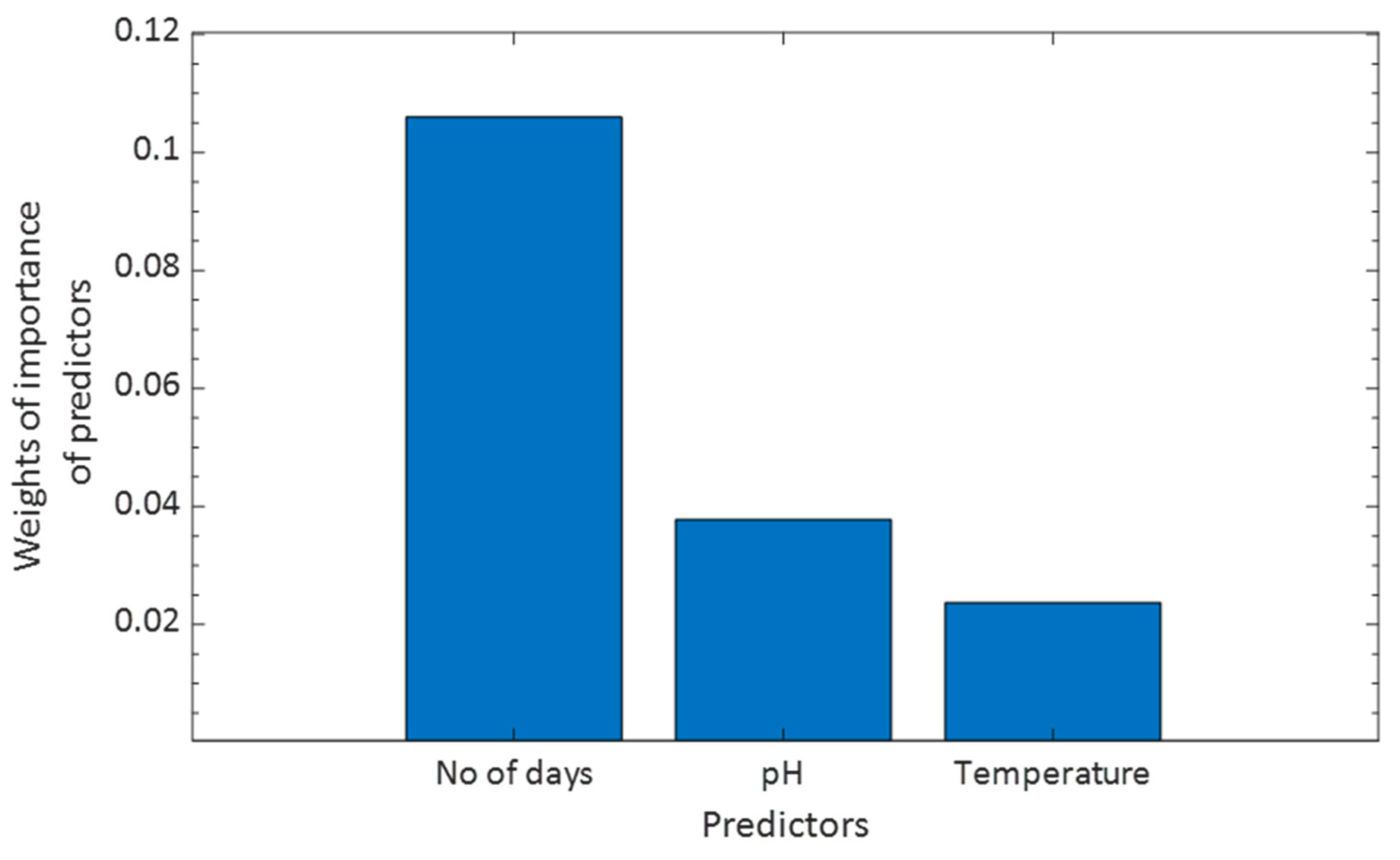
• To employ the reliefF statistical test in ranking of the predictors into weights of importance to the total viable bacteria counts.
• To develop a non-linear response surface model to predict the total viable bacteria counts with the number of days, daily slurry temperatures and pH as the predictors.
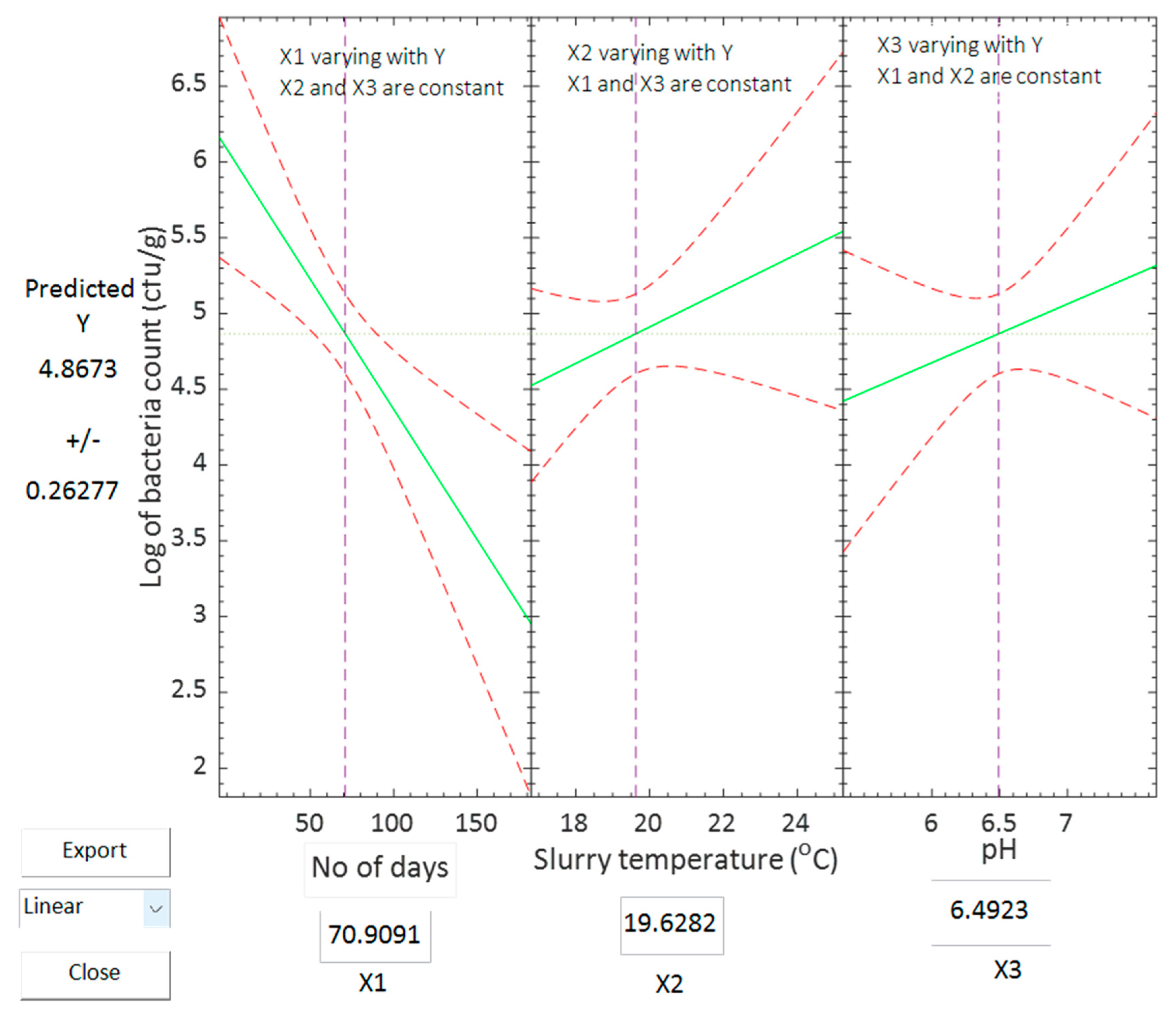
• To simulate the variation in the total viable bacteria counts with each of the predictor, whereas the other input parameters are held constant using the 2D multi-contour surface plots.
• To perform a robust validation of the developed model used in the prediction of the total viable bacteria counts.

1.4. Research Questions of the Study

The following formulated research questions for the study include:

• Can a data acquisition system be designed and built to measure the ambient and physicochemical parameters, quality, and quantity of potential biogas production in a balloon-type digester?
• Can the input parameters (number of days, slurry temperature, and pH) influence the total bacteria counts, and is it possible to rank them according to their weights of importance?
• Can a response surface model be developed that could be used to predict the total bacteria counts in a balloon digester using the number of days, slurry temperature and pH as the predictors.
• Can a 2D multi-contour surface plots be generated to simulate the variation in each of the input parameter with the model output while the others are held constant?
• Can the derived response surface model of the balloon digester fed with cow waste be accurately validated?

1.5. Delineation of the Study

The study was only conducted in one province and in one place (at the Physics Research Centre-University of Fort Hare, Alice campus) in South Africa, and utilized cow manure as the feedstock for the balloon digester. The designed and analysis of the experimental balloon digester was not taking into consideration in the study. The study utilized a fabricated heat-seal plastic balloon digester with maximum volume capacity of 8 m² according to manufacturers’ specifications.

2. Methodology of the Study

The study methodology encompassed both experimental setup and methods to assist in the determination of the critical measurements and development of the mathematical model in a bid to achieve the objectives.

2.1. Materials and Experimental Setup

Table 1. Materials and sensors used in the study.

Devices and Materials Employed in Both the Physical and Chemical Analysis
Item	Device and Materials	Quantity
1	Centrifugal tubes	10
2	Nessler’s reagent	-
3	Hexios, Thermo-Spectronics Spectrometer	1
4	Distilled water	-
5	Dish	1
6	Electric oven	1
7	PHH-SD1 pH meter	1
8	TMC6-HD copper pipe temperature sensors	4
9	Portable biogas analyzer, IRCD4	1
10	Tryptic soy broth medium	-
11	Physical saline	-
12	Triplicates of microbiological media (nutrient agar and anaerobic agar)	-
13	Fridge	1
14	Incubator	1
15	Weight balance	1
16	muffle furnace	1
B.  Devices, Sensors and Materials Used in the Experimental Setup
Item	Device and Materials	Quantity
1	Fabricated balloon digester	1
2	Feedstock of cow waste (slurry)	2500 L
2	An open surface concrete structure	1
3	A black wooden board (insulation cover)	1
4	Portable biogas analyzer, IRCD4	1
5	TMC6-HD copper pipe temperature sensors	4
6	Hobo-UX120 four external channel data logger	1
7	PHH-SD1 pH meter	1
8	Slurry measuring cylinder (250 cm3)	1
9	ZAN-TECHS gas flow meters with data logger	1
10	Control flow valve	1
11	Biogas circulation pump	1
12	Connecting biogas tubing	1
13	Biogas collection chamber	1
14	Weatherproof data loggers’ enclosure	1
15	A zinc roof open structure (re-forcing protection of sensors and system)	1

shows the materials, sensors, data loggers and technological device used in the study. The temperature sensors were of copper pipe and the temperature ranged from −20 to 75 °C, whereas the pH sensors recorded measurement was between 1 and 14. All the sensors and transducers were calibrated before installed at designated location in the balloon digester to read the appropriate measurements.

The balloon digester was accommodated within a concrete structure of 8 m³ by volume and partition into three sectors including the influent tank of dimension 0.95 m by 0.89 m by 0.83 m, a bioreactor tank of length 3.25 m and width 2 m and the effluent tank of 1.2 m³ by volume. Figure 3 shows a detail schematic diagram of the balloon digester embedded in a concrete structure and the installed temperature sensors, gas flow transducer and pH electrode installed at specific location of the balloon digester and the different data loggers are housed in a weatherproof enclosure. Five consecutive days (26–30 June 2015) were used to feed the balloon digester with a uniform mixture of dairy cow waste and water in the ratio 1:1. The adopted mixing ratio of the cow waste to water to prepare the slurry was determined with referenced to the moisture content of the waste. The physicochemical parameters (pH, moisture, % of total solids, % of volatile solids, ammonium level and % of ash content) of the undigested waste were determined before the preparation of the slurry. The bottom and middle temperature sensors (labelled 1 and 2) measured the average temperature of the slurry, whereas the temperature sensors within the biogas region in the balloon digester (labelled 3) and in the vicinity of the digester (labelled 4) measured the temperature of the biogas and ambient temperature. All the temperature sensors were connected to an external four-channel data logger (labelled 5). The pH electrode (labelled 25) was inserted in the slurry and connected to the pH meter (labelled 24), which stored the measured pH of slurry. The biogas flow meter (labelled 8) was installed along the connecting tubing transporting the biogas produced from the digester (labelled 18) to the biogas collection chamber (labelled 22) upon opening of the control valve at the end of the anaerobic digestion process. The cumulative volume of the biogas was measured and stored in the biogas flow data logger (labelled 9). The transducer of the biogas analyzer (labelled 6) sense and analyzed the composition and percentages of the biogas (methane and carbon dioxide) produced from the anaerobic digestion in the digester and were stored in the biogas analyzer (labelled 7). The open and close control valve (labelled 19) regulates the flow rate of biogas from the digester to the biogas collection chamber which occurred at the end of the retention time. The gas circulation pump (labelled 21) assists to provide the appropriate pressure for biogas to be transported from the digester to the biogas collection chamber. The digester was monitored for six months (July–December 2015) while operating in a batch mode. Samples were withdrawn on a daily basis for analysis of the microbial loads, whereas the pH and temperatures of the slurry were continually monitored in one-minute intervals and the average day values determined throughout the retention period.

2.2. Methods

2.2.1. Raw Anaerobic Digestion Material (Cow Manure)

Equal volumes of five samples of the fresh cow manure (labelled sample A, sample B, sample C, sample D, and sample E) with a cumulative volume of 2500 L were obtained from the Fort Hare Diary Farm, Alice, over consecutive weekdays (26–30 June 2015).

2.2.2. Physicochemical Analysis of the Slurry Samples

• Calculation of the ammonium (NH4) level of the sample

Ziganshin el al.’s [41] method was employed in the determination of the ammonium level. Each of the five samples were centrifuged at the rate of 2000× g in 20 min and the supernatant was decanted and colored with Nessler’s reagent in accordance with the procedure of Manyi-Loh et al. [42]. The wavelength of the absorbance of the colored solutions was determined to be 425 mm with the used of Hexios, thermo-spectronics spectrometer. The calculation of the ammonium level was performed by applying the standard (ammonia solution) with a concentration of 0.909 g/mL. On the other hand, distilled water was utilized as a blank to neutralize the absorbance of water in the samples and standard.

ii.

Determination of percentage of moisture content of samples

The percentage of total moisture content were determined by the APHA method as used by Fridh et al. [43]. The method involved the weighing of samples in a dish and drying in an oven at a temperature of 105 °C overnight. Both the weight of the dish and sample before drying and that of the dish and sample after drying were measured with a mass balance. The percentage of the moisture content was evaluated by Equation (1).

$$\% \mathrm{moisture} \mathrm{content}=\frac{\left({\mathrm{m}}_2-{\mathrm{m}}_1\right)-\left({\mathrm{m}}_3-{\mathrm{m}}_1\right)}{\left({\mathrm{m}}_2-{\mathrm{m}}_1\right)}\times 100$$

1

where ${\mathrm{m}}_1$= mass in grams of empty dish, ${\mathrm{m}}_2$= mass in grams of sample and empty dish before drying, ${\mathrm{m}}_{3 }$= mass in grams of sample and empty dish after drying.

iii.

Determination of percentage of dry matter (total solids)

The percentage of total solids were determined by the APHA method as employed by Bradley’s formulation [44]. The method involved the determination of the weight of a sample (W_S) in a dish and again measured the weight of the dry matter (W_DM) after drying at 105 °C in an oven over a 24 h period. The percentage of the total solids is given in Equation (2).

$$\% \mathrm{total} \mathrm{solids}=\frac{{\mathrm{W}}_{\mathrm{DM}}}{{\mathrm{W}}_{\mathrm{S}}}\times 100$$

2

where, ${\mathrm{W}}_{\mathrm{DM}}=$ weight of dry matter and ${\mathrm{W}}_{\mathrm{s}}=$ weight of sample

iv.

Determination of percentage of volatile solid content and ash content

After the determination of the total solids, the overnight dried sample achieved was combusted using a muffle furnace at 550 °C for 1 h period. The residual weight of ash and the dish was recorded, and the percentage of volatile solids was derived by Equation (3).

$$\% \mathrm{volatile} \mathrm{solid}=\frac{\left({\mathrm{W}}_{\mathrm{DM}}-{\mathrm{W}}_{\mathrm{ash}}\right)}{{\mathrm{W}}_{\mathrm{DM}}}\times 100$$

3

where ${\mathrm{W}}_{\mathrm{DM}}$= weight of dry matter and dish and ${\mathrm{W}}_{\mathrm{ash}}$ = weight of ash and dish

In addition, the percentage of ash content was obtained from Equation (4) as used by Van Wychen [45].

$$\% \mathrm{ash} \mathrm{content}=\left(\frac{\left({\mathrm{m}}_4-{\mathrm{m}}_1\right)}{\left({\mathrm{m}}_2-{\mathrm{m}}_1\right)}\times 100\right)\times \frac{100}{100-\%moisture}$$

4

where m₁ = mass in grams of empty dish, m₂ = mass in grams of sample and empty dish before drying, m₄ = mass in grams of ash and empty dish after drying.

The physicochemical characterization of the waste is shown in

Table 2. Sample characterization based on utilizing feedstock of cow manure.

Parameters	Sample A	Sample B	Sample C	Sample D	Sample E	Mean	Standard Deviation
Percentage of moisture content	89.12	91.23	91.19	89.96	90.78	90.38	0.886 $\pm$ 0.396
Percentage of total solids	10.88	8.77	8.81	10.04	9.22	9.55	0.975 $\pm$ 0.436
Percentage of volatile solids	65.76	68.25	72.65	71.55	73.04	70.25	3.138 $\pm$ 1.403
Percentage of ash content	34.24	31.75	27.35	28.45	26.96	29.75	3.138 $\pm$ 1.403
Ammonium (NH4) level (mg/mL)	2.19	2.01	2.25	2.28	2.20	2.18	0.105 $\pm$ 0.046
pH	6.83	6.82	6.59	6.76	6.46	6.69	0.162 $\pm$ 0.072

. The study was conducted over a six-month period (July to December 2015) at the Renewable Energy Centre, under the Physics department, University of Fort Hare, Alice campus.

v.

Determination of pH, ambient temperature, slurry temperature and biogas yield

The average daily ambient temperatures were measured by the hobo copper pipe temperature sensor (labelled 4) and the slurry temperatures were measured by the hobo copper pipe temperature sensors (labelled 1 and 2). All the temperature sensors were connected to a hobo four-external channel data logger (labelled 5). The pH of slurry was measured by the pH electrode (labelled 25) inserted at the bottom of the digester and the recorded pH was stored in the PHH-SD1 pH meter (labelled 24), which is connected to the pH electrode by specialized cables. The percentages of the composition of the biogas produced were sensed by the transducer (labelled 6) and analyzed by the portable biogas analyzer, IRCD4 (labelled 7) at the end of the retention time and the average quality of methane and carbon dioxide were 65.8% and 31.2%. The cumulative volume of biogas produced over the six months hydraulic retention time (July to December 2015) was measured by the biogas flow meter (labelled 8) and stored in the data logger ZAN-TECHS gas flow data logger (labelled 9). Furthermore, triplicate determination was conducted on each of the daily collected samples of slurry.

vi.

Microbial analysis of samples

The method employed by Sahlström [46] was used to determine the total viable bacteria counts for the undigested and withdrawn samples during digestion of the slurry. Each sample was aseptically collected and poured into a tryptic soy broth medium in sterile centrifuge tubes for onward transportation to the laboratory based on best practices. The samples were analysed immediately once arrived the laboratory. The determination of the total viable bacteria counts was conducted following the procedure provided below. 1 g of each sample was consecutively diluted tenfold in 9 mL of sterile saline. The range of dilution of 10⁻¹–10⁻⁵ was spread in triplicates in different microbial media (nutrient agar to obtain total aerobic bacteria counts and anaerobic agar to obtain total anaerobic bacteria counts). Above all, the inoculated plates were incubated at 37 °C for 24 h for the aerobic and anaerobic bacteria counts. At the end of the incubation, the number of emergent colonies on each plate were counted and recorded with each value representing the average of the triplicate plating in accordance with the method used by Bodhidatta et al. [47].

2.2.3. Statistical Analysis

The analytical analysis and statistical tests were conducted with the MATLAB software version 2021a following standard methods [48]. The one-way analysis of variance (ANOVA) test was utilized to check on any significant difference between the test data of the targets and the model outputs as well as the validated data of the targets and the predicted values that were obtained with the derived mathematical model (non-linear response surface model) with referenced to the p-values and the generated ANOVA plots [49,50]. The reliefF algorithm was employed to rank the contribution of the predictors (number of days, daily slurry temperature and pH) according to the weight of importance to the desired targets (log of total viable bacteria counts) [51].

2.2.4. Development of Non-Linear Response Surface Model

A non-linear response surface model was developed using the number of days (x1), daily slurry temperature (x2) and pH (x3) as the predictors, whereas the log of total viable bacteria counts (y) was the desired response. The reliefF algorithm was employed to rank the contribution of the predictors (number of days, daily slurry temperature and pH) according to the weights of importance to the output (log of total viable bacteria counts) [52]. The determination coefficient, root-mean-square error and p-value were used to test the accuracy of the model with reference to the predictions (model outputs) and the targets (experimental determined log of total viable bacteria counts) [53]. Two-dimensional multi-contour surface plots were developed to simulate the production of the total viable bacteria counts with each of the predictors using the developed response surface model.

The response surface model used to predict the log of the total viable bacteria counts with the number of days, daily slurry temperature, and pH as predictors was a non-linear fitting model. The mathematical model equation for the response surface model is given in Equation (5).

$$\mathrm{y}=\frac{{\mathsf{\beta }}_1\mathrm{x}2-\mathrm{x}3/{\mathsf{\beta }}_5}{1+{\mathsf{\beta }}_2\mathrm{x}1+{\mathsf{\beta }}_3\mathrm{x}2+{\mathsf{\beta }}_4\mathrm{x}3}$$

(5)

where y = log of total viable bacterial counts in unit [cfu/g], x1 = Number of days, x2 = daily slurry temperature in unit [°C], x3 = pH and ${\mathsf{\beta }}_1$= scaling constant for x2 in unit [cfu/g°C], ${\mathsf{\beta }}_2$= Scaling constant for x1 with the unit [/day], ${\mathsf{\beta }}_3$ = Another scaling constant for x2 in unit [/°C], ${\mathsf{\beta }}_4=$ Scaling constant for x3 with no unit and ${\mathsf{\beta }}_5$ = Another scaling for x3 with no unit.

The mathematical model was developed in MATLAB and by considering the modelled equation as the optimization function, whereby y represented the desired response (log of total viable bacteria counts) and x1, x2 and x3, represented the predictors (number of days, daily slurry temperature and pH, respectively), whereas ${\mathsf{\beta }}_1$, ${\mathsf{\beta }}_2$, ${\mathsf{\beta }}_3$, ${\mathsf{\beta }}_4$ and ${\mathsf{\beta }}_5$ were the given scaling constants attributed to specific input variables. The values of the scaling constants are determined by performing a non-linear function optimization with the modelled equation as the optimization function using the trained (testing) data set for both the input and output parameters obtained from the experimental measured data. The optimization algorithm was implemented by choosing initial values for the input and output parameters. A computation iteration was executed by running the optimization function with the chosen initial values as the initial condition. The iteration stops when the model outputs (predicted log of total viable bacteria counts (yp) mimic with very high accuracy the actual targets (determined log of total viable bacteria counts (yo)) and the correct scaling values of each of the scaling constants were computed.

Table 3. Input and output parameters of the developed response surface model.

Input Parameters	Input Symbols	Scaling Attribute	Scaling Values	Output
Forcing constant			1	Log of total bacteria counts (y) r2 = 0.959, RMSE = 0.197, p-value = 0.602
Number of days	x1	${\mathsf{\beta }}_2$	0.0047
Daily slurry temperature	x2	$$\begin{gathered} {\mathsf{\beta }}_1 \\ {\mathsf{\beta }}_3 \end{gathered}$$	0.4947 0.0521
pH	x3	$$\begin{gathered} {\mathsf{\beta }}_4 \\ {\mathsf{\beta }}_5 \end{gathered}$$	−0.1445 2.2002

shows the inputs and output parameters as well as the scaling values derived from the developed response surface model. The input variable x1 was associated with a single scaling attribute (${\mathsf{\beta }}_2$) and x2 was assigned with two scaling constants (${\mathsf{\beta }}_1$ and ${\mathsf{\beta }}_3$), whereas x3 was attributed with two scaling constants (${\mathsf{\beta }}_4$ and ${\mathsf{\beta }}_5$). The determination coefficient, the rootmean square error and the p-value between the targets (yo) (testing samples) and the predicted log of total viable bacteria counts (yp) were 0.959, 0.197, and 0.602, respectively. The high value of the determination coefficient, which is closed to 1, is an indication that the developed non-linear response surface model demonstrates a very good agreement between the predicted outputs (yp) and the targets (yo). The large p-value (0.602 which is greater than 0.05, was obtained between the predicted outputs (yp) and the targets (yo) and confirmed that there was no significant difference between the two groups within a 95% confidence level. The root mean square error between the predicted outputs and the targets was smaller than the minimum value of the actual targets. Therefore, the condition for accepting and utilizing the developed response surface model is fulfilled.

2.3. Measurement Accuracies and Uncertainties

The determined uncertainties from the calculated parameters with respect to the determined error measurements based on the set of independent variables, is derived from Equation (6) [54,55].

$${\mathrm{w}}_{\mathrm{r}}={\left[{\left[{\mathrm{w}}_1\frac{\partial \mathrm{R}}{\partial {\mathrm{X}}_1}\right]}^2+{\left[{\mathrm{w}}_2\frac{\partial \mathrm{R}}{\partial {\mathrm{X}}_2}\right]}^2+\dots \dots \dots \dots +{\left[{\mathrm{w}}_{\mathrm{n}}\frac{\partial \mathrm{R}}{\partial {\mathrm{X}}_{\mathrm{n}}}\right]}^2\right]}^{\frac{1}{2}}$$

(6)

where $\mathrm{R}$ = the given function; ${\mathrm{w}}_{\mathrm{r}}$ = total uncertainty; ${\mathrm{X}}_1,{ \mathrm{X}}_2, \dots \dots .{\mathrm{X}}_{\mathrm{n}}$ = independent variables and ${\mathrm{w}}_1,{ \mathrm{w}}_2, \dots \dots .{\mathrm{w}}_{\mathrm{n}}$ = uncertainty in the independent variables, $\frac{\partial \mathrm{R}}{\partial {\mathrm{X}}_{\mathrm{n}}}$ = partial fraction term and ${\mathrm{w}}_{\mathrm{n}}\frac{\partial \mathrm{R}}{\partial {\mathrm{X}}_{\mathrm{n}}}$ = uncertainty term.

The type A uncertainties are measured from the statistical means and standard deviations obtained from the recorded measurements [56] and are shown in

Table 4. Uncertainties of the measured and derived quantities.

Quantity	Type A Uncertainty	Type B Uncertainty	Combined Uncertainty
Ambient temperature (°C)	±0.200	±0.120	±0.320
Biogas flow rates measurements (L/min)	±0.010	±0.006	±0.016
pH measurements	±0.130	±0.003	±0.133
Slurry temperature (°C)	±0.200	±0.120	±0.320
% Total solids content	±0.850	±0.105	±0.955
% Total volatile content	±0.850	±1.405	±2.255
% Ash content	±0.850	±1.203	±2.053
Ammonium level (mg/mL)	±0.060	±0.020	±0.080

. In addition, the type B uncertainties are linked to the accuracy of the sensors or by the utilization of Equation 6 to obtain the derived uncertainty of the quantities (% total solids, % volatile solids, and % ash content). Table 4 shows the combined uncertainties of the prescribed quantities (both type A and type B uncertainties).

3. Results and Discussion

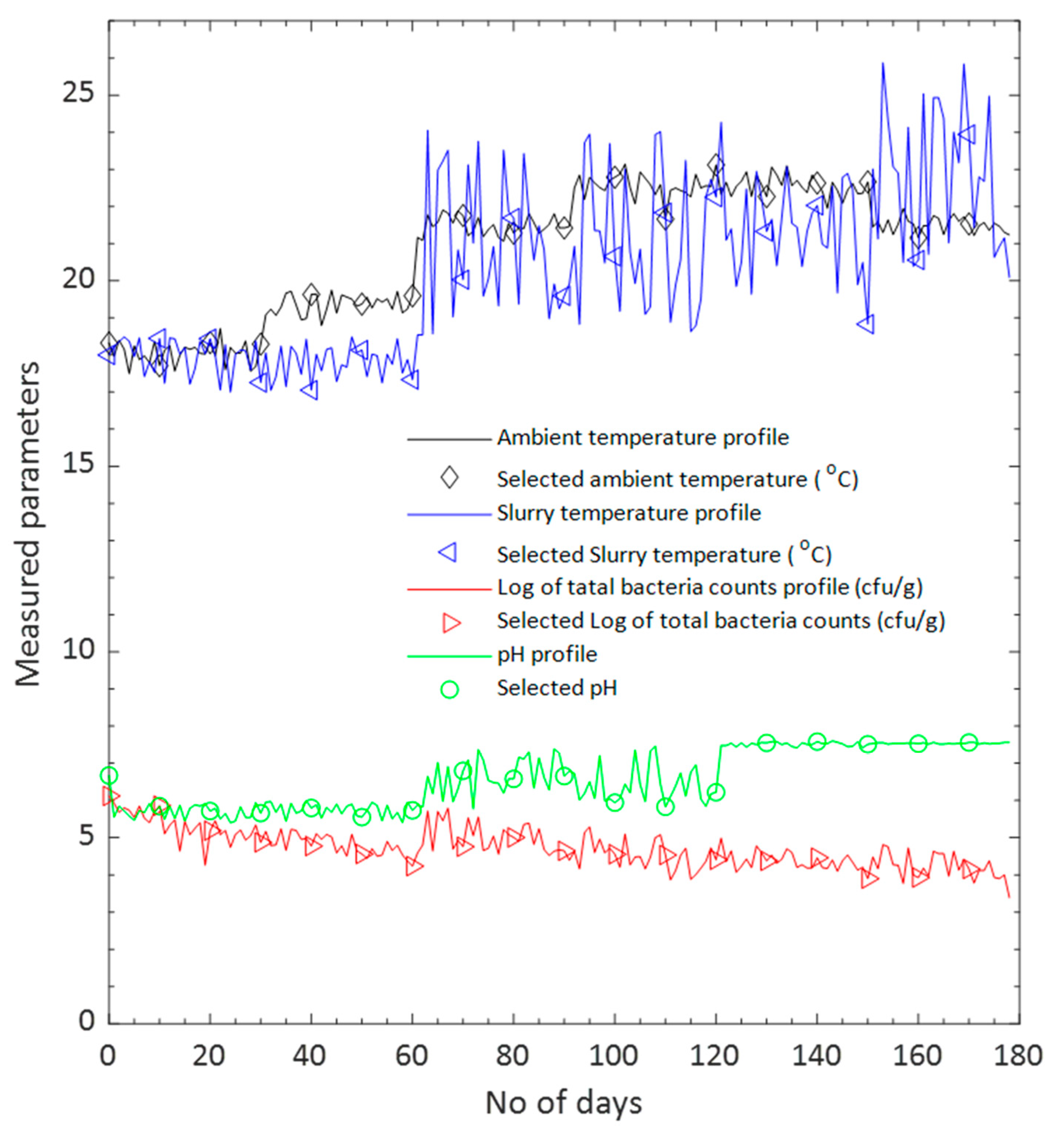
3.1. Profiles of Ambient Temperature, Input and Output Parameters during Anaerobic Digestion

The variation of the daily average ambient temperature, daily slurry temperature, pH and log of total viable bacteria counts are shown in Figure 4. The figure shows the daily profiles as line graphs and the selected data points in 10-day intervals for each parameter. The dynamics of the weather condition, the input and output parameters demonstrated continual variation during the anaerobic digestion process. Despite the fact that the daily slurry temperature of the digester may be influenced by ambient temperature, the profiles of the average daily ambient temperature and daily slurry temperature showed some degree of correlation. However, the slurry temperature does not solely depend on the ambient temperature as other physicochemical factors are capable of impacting the slurry temperature. It was observed that the anaerobic digestion process occurred in two regimes. The first regime was associated with the psychrophilic process (<20 °C) for the first 60 days (two months), whereas in the second regime the process was mesophilic (20 °C < slurry temperature < 30 °C) for the remaining 119 days (4 months). These results agree with the findings by Cioabla et al. [57]; however, the authors conducted their research using agricultural vegetable residues. Again, it was depicted that during the psychrophilic regime, the daily ambient temperature, slurry temperature, and pH fluctuated between 18.1 and 21.2 °C, 17 and 19.23 °C, and 5.4 and 5.85, respectively, whereas the log of total viable bacteria counts ranged from 5.00 and 6.02 cfu/g. Furthermore, in the mesophilic regime, the daily ambient temperature, slurry temperature, and pH varied between 21.04 and 22.58 °C, 20.9 and 25.5 °C, and 6.1 and 7.67, respectively, whereas the log of the total viable bacteria count was in the range of 3.38 to 5.40 cfu/g.

3.2. Characteristics of the Cow Manure and Variation of Physicochemical Parameters

The results achieved from Table 2 based on the percentage of total solids, total volatile solids and ash content justified that the cow waste possessed substantial biodegradable constituent with the capability of undergoing digestion by the microorganisms in the anaerobic digester to generate biogas. Figure 4 revealed that at the initial state before the commencement of charging, the total aerobic and anaerobic counts were very high. These results affirmed that the cow manure is a favourable feedstock (substrate) of biogas production since the rumen microbes are of vital importance in anaerobic digestion, which is responsible for the degradation of the organic composition of the cow waste [58]. The high level of microbial loads showed in Figure 4 justified public health control measures needing to be reinforced as the cow dung can act as a potential source of water and soil pollution. The failure to treat the cow waste before it was released into the environment can act as a high risk and a potential source of both soil and water pollutions. The absolute present of the high microbial loads in the cow waste is enough reason for a call of concerned. The high microbial loads served as an eminent threat to living animals and humans since infection is likely probable due to the mode of transmission, which is very feasible [59]. More so, the enhancement of the performance of anaerobic bacteria is governed by the temperature and pH of the digester substrate. The waste from livestock, especially dairy cow waste, has been proven to have high buffering alkaline potential when digested by microorganisms [60]. It is of crucial importance to mention that during the monitoring period, the pH of the digester remains uncontrolled. The figure shows that during the first two months of the anaerobic digestion, there was a decrease in the pH medium (pH drop from 6.60 to 5.85) and may be accounted to the high concentration of volatile fatty acids, bicarbonate alkalinity and carbon dioxide which are the results of the end products of the first and second phases of the anaerobic digestion process (hydrolysis and acidogenesis. The findings are in support with most of the studies conducted on the performance of anaerobic digestion in the balloon digester, whereby as the process progresses, the volatile fatty acids metabolize, and the pH eventually increases to the appropriate buffering level (neutral pH), favourable to produce the biogas. Research has revealed that both acidogenic- and methanogenic-forming bacteria have their optimum pH for metabolism [61]. The methanogens are extremely sensitive and thrive efficiently within the pH ranged from 6.6–7.6 [62]. Alternatively, the metabolic rate of microorganisms is impacted by the temperature and is capable of altering the effectiveness of the anaerobic microbes responsible for the process of biogas production. Lastly, Figure 4, shows that the daily variation in the slurry temperature during the duration of anaerobic digestion was not significantly affected by the ambient temperature. The profile revealed the existence of two regimes (psychrophilic process (temperature < 20 °C) occurring during the first two months and mesophilic regime (20 °C < slurry temperature < 30 °C) during the last four months of the anaerobic digestion [63].

3.3. ReliefF Test Used in Weight Ranking of the Predictors to the Total Viable Counts

A reliefF test is a statistical technique used to rank predictors according to their weights of importance to the desired response (targets) using parametric regression method. The reliefF algorithm was executed in MATLAB by applying the command [Rank Weight] = relieff(x,y,k), which returns the order of ranking of the predictors and their corresponding weights of importance to the desired response. The quantity x and y represent the predictors and output, whereas k is the number of potential predictors (x) influencing the output (y) and by default was set to 10. It is important to point out that the weights can range from −1 to 1. A negative weight ascribed to predictor insinuate the input parameter was a secondary factor, whereas positive weight attributed to input parameter revealed it is a primary factor. The more positive the weight value implied the input parameter would significantly contribute to the desired response. Figure 5 shows a bar chart of the predictors (number of days, slurry temperature and pH) and the weights of importance to the desired output (log of total viable bacteria counts). It was observed that all the predictors were primary factors with the number of days contributing the most by weight (0.106), followed by pH (0.038 and the least was daily slurry temperature (0.024).

3.4. 2D Multi-Contour Surface Plots to Simulate the Variation in the Response with Each Predictor

The 2D multi-contour surface plots are two-dimensional multiple plots developed from a derived mathematical model to simulate the variation in the output with a specific input parameter, whereas the others are held constant. Each of the two-dimensional plots represents the predictors on the x-axis and the predicted output on the y-axis. A solid graph (line or curve) is used to demonstrate the variation of the desired response with changes in the specific input parameter, whereas the other input parameters are unchanged. The two broken graphs (lines or curves) between the solid graph represent the 95% confidence bounds [64].

Two-Dimensional Multi-Contour Plots with the Developed Non-Linear Response Surface Model

Figure 6 shows the 2D multi-contour surface plots of the predictors (number of days (x1), daily slurry temperature (x2) and pH (x3)) and the predicted output (log of total viable bacteria counts (Y). The green solid graphs showed the rate of changed of the predicted output (Y) with a specific predictor, whereas the other predictors are invariant. The red broken graphs between the solid green graphs represent the 95% confidence bounds. The simulated 2D multiple plots of the predicted total viable bacteria counts (Y) with the number of days (x1), whereas the other two predictors are held constant (x2 = 20 °C, and x3 = 6.5) showed that the rate of changed of predicted log of total viable bacteria counts with the number of days was negative. The green solid curve was approximated to a best linear-fit graph with negative slope of $-0.0146$ cfu/g/day. The rate of change of the predicted log of total viable bacteria counts (Y) with daily slurry temperature (x2) while the predictors (x1 = 71 and x3 = 6.5) are held unchanged, can be approximated to a best-fit line graph with a slope of 0.1205 cfu/g/°C. In addition, the rate of changed of the predicted log of total viable bacteria counts (Y) and pH (x3) with the predictors (x1 = 71 and x2 = 20 °C) staying unchanged, can be approximated to a straight-line graph with a positive slope of $0.1771$ cfu/g.

Table 5. Design experimental results from simulated 2D multi-contour surface plots using the developed model (daily slurry temperature and pH constant (x2 = 20 °C and x3 = 6.5)).

Chosen Input x1 (Number of Days)	Predicted y with Non-Linear Model (Log of Bacteria Counts)	Derived Equation with Non-Linear Model $(\mathit{y}=-0.0146\mathit{x}1+5.9430)$
10	6.036
30	5.580
50	5.188
70	4.847
90	4.548
110	4.284
130	4.049
150	3.839
170	3.649

shows the design simulated results of sample data set obtained from the generated 2D multi-contour surface plots of number of days (x1) and the predicted log of total viable bacteria counts (Y) with x2 = 20 °C and x3 = 6.5 remaining unchanged. It was observed that as the values of x1 increases, the values of Y decreased with the slope equal to $-0.0146$ cfu/g/day and was derived from the approximated best-fit linear equation shown in Table 5.

Table 6. Design experimental results from simulated 2D multi-contour surface plots using the developed model (number of days and pH held constant (x1 = 71 and x3 = 6.5)).

Chosen Input x2 (Daily Slurry Temperature)	Predicted y with Non-Linear Model (Log of Bacteria Counts)	Derived Equation with Non-Linear Model $(\mathit{y}=0.1649\mathit{x}2+1.519)$
17	4.277
18	4.482
19	4.672
20	4.842
21	5.010
22	5.162
23	5.305
24	5.438
25	5.563

shows the design simulated results for the sample data set obtained from the generated 2D multi-contour surface plots of daily slurry temperature (x2) and the predicted log of total viable bacteria counts (Y whereby x1 = 71 and x3 = 6.5 remained unchanged. It was depicted that as the values of x2 increased, the values of Y increased with the gradient equal to $0.1205$ cfu/g/day, as derived from the approximated linear equation shown on the table.

Table 7. Design experimental results from simulated 2D plots using the developed model (number of days and daily slurry temperature held constant (x1 = 70 and x2 = 20 °C)).

Chosen Input x3 (pH)	Predicted y with Non-Linear Model (Log of Bacteria Counts)	Derived Equation with Non-Linear Model $(\mathit{y}=0.1771\mathit{x}3+3.701)$
5.50	4.691
5.75	4.727
6.00	4.765
6.25	4.805
6.50	4.847
6.75	4.891
7.00	4.938
7.25	4.987
7.50	5.038

shows the design simulated results of the sample data set obtained from the produced 2D multi-contour surface plots of pH (x3) and the predicted log of total bacteria counts (Y) whereby x1 = 71 and x2 = 20 °C are held constants. It was revealed that increasing the values of x3 can results in increased in the values of Y and the gradient was $0.1771$ cfu/g, derived from the approximated linear equation shown on the table.

3.5. Testing of the Accuracy of the Developed Model

The data set of the input and out parameters during the six months (179 days) of hydraulic retention time of the anaerobic digestion of cow waste in a balloon digester were randomly split into testing and validation samples in the ratio of 60 and 40%, respectively. The data set (107 testing samples) of the measured input parameters (number of days, daily slurry temperature and pH), were used in the derivation of the non-linear response model to determine the predicted outputs (predicted log of total viable bacteria counts) called the model outputs, whereas the 107-sample data of the experimental determined log of total viable bacterial counts were used as the targets. The targets and the model outputs were compared to verify the accuracy of the developed model with reference to the determination coefficient, root mean square error and the p-value.

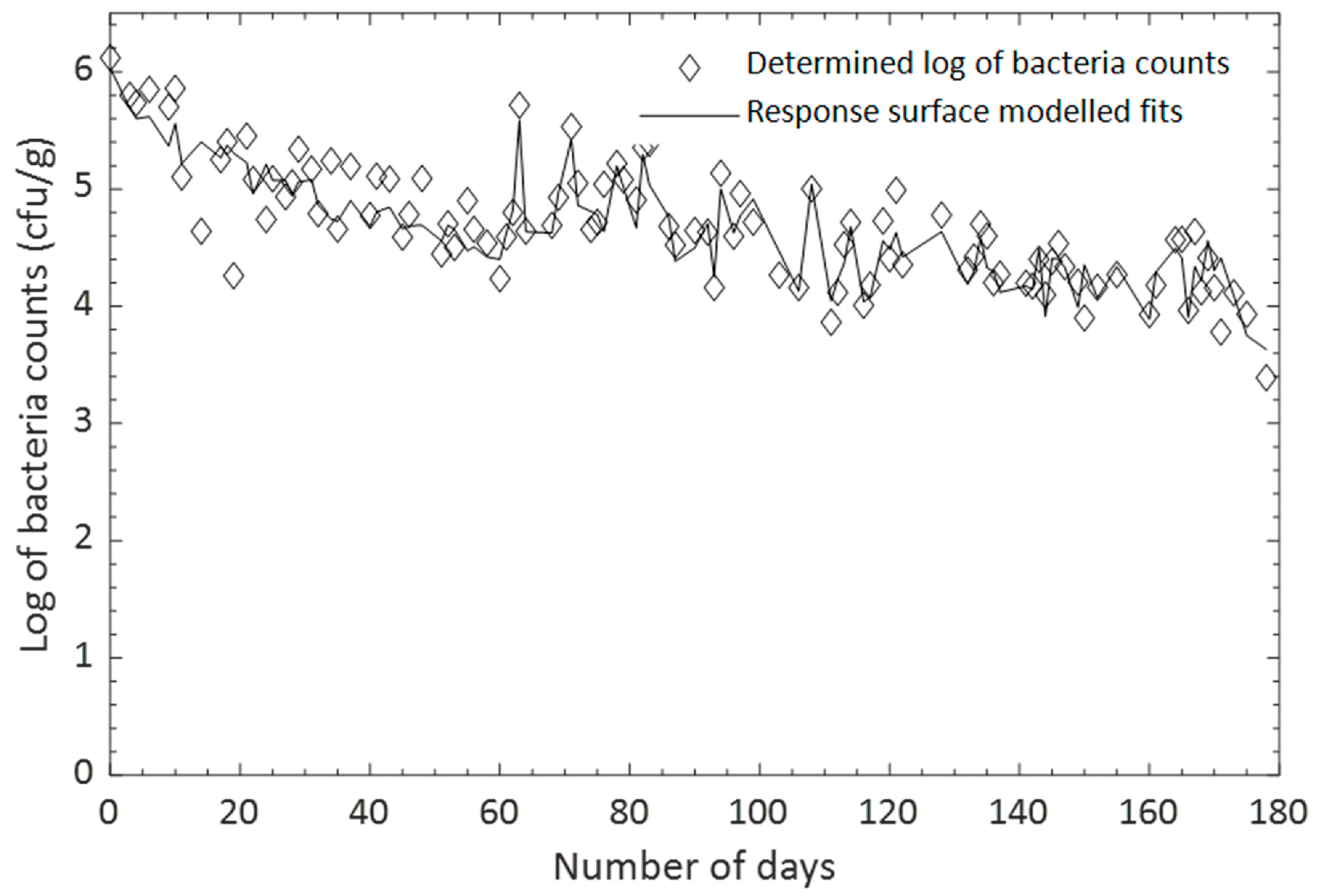
3.5.1. Testing of the Accuracy of the Developed Non-Linear Response Surface Model

Figure 7 shows the sample data of the determined log of total viable bacteria counts (targets) and the modelled best curve-fit using the developed response surface model (model outputs). It was observed that the model outputs accurately predict the targets. The determination coefficient, root mean square error and p-value between the targets and model outputs were 0.959, 0.197 and 0.602, respectively. The determination coefficient was very good and closed to 1, whereas the root mean square error was closed to 0 and much smaller than the minimum value of the experimental determined targets. The p-value was significantly greater than the threshold value (0.05), which confirmed that no significant difference exists between the targets and the model outputs. The data set of both the targets and model outputs obeyed normal distributions with no outliers. Therefore, the very good values of the determination coefficient, root mean square error and p-value were adequate to accept the developed model in the prediction of the log of total viable bacterial counts.

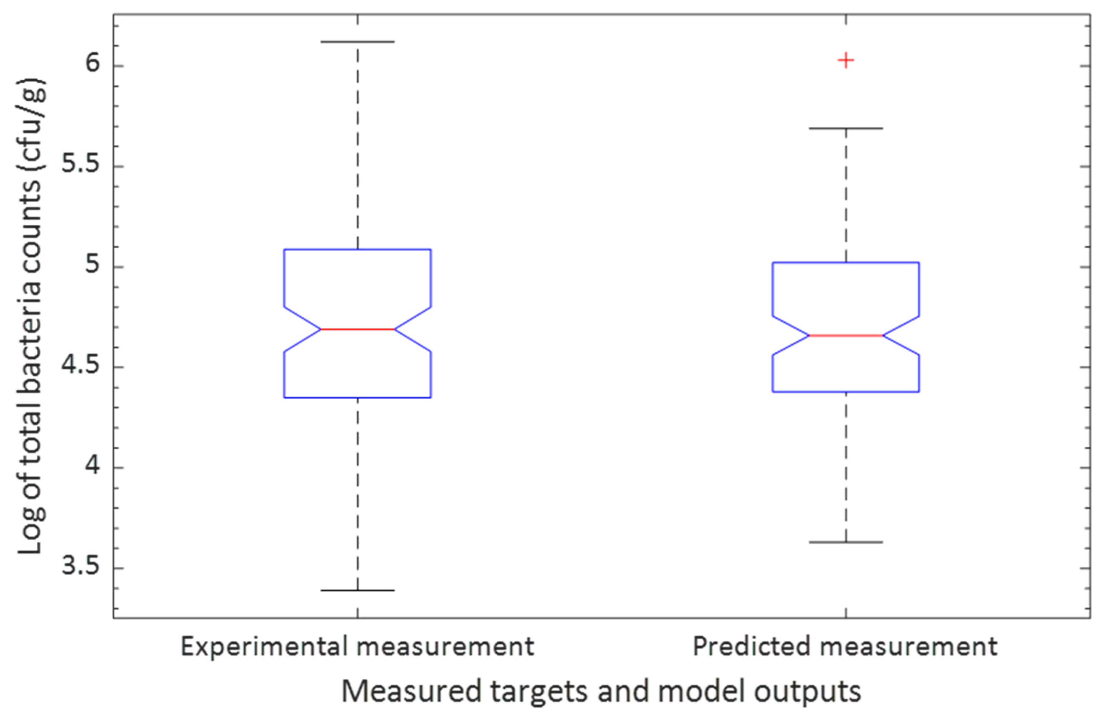
3.5.2. ANOVA Statistics to Confirm the Accuracy of Developed Non-Linear Response Surface Model Using Testing Data Set

Table 8. ANOVA table for the testing data set of targets and model outputs.

Statistics Based on Targets and Model Outputs with the Response Surface Model
Source	Sum of Square (SS)	Degree of Freedom (df)	Mean Square (MS)	F	Prob > F
Columns	0.0674	1	0.0674	0.27	0.602
Error	53.2762	216	0.2467
Total	53.3436	217

shows the ANOVA table for the targets (experimental determined log of total viable bacteria counts) and the model outputs derived from testing data sets of the input parameters. The columns and error under the source represented the between groups (columns = 2) and within groups (error = 216). The degree of freedom within columns is equal to the number of between groups minus 1 (columns −1) and was equal to 1. The degree of freedom of the error is equal to the degree of freedom within the groups and was equal to 216. The total degree of freedom is the sum of degree of freedom between columns and errors and was 217. The groups of targets and model outputs revealed that the mean square of the columns, which is the ratio of the sum of square and the degree of freedoms for columns was 0.0674 (0.0674/1), whereas the mean square of the error is the ratio of sum of square and the degree of freedom for error and was 0.2467 (53.2762/216). The ratio of the mean square of the columns and error was 0.27 (0.0674/0.2467) and was equivalent to the F-statistic. The p-value is equal to the probability of the F-statistic and was 0.602. The p-value (0.602) is significantly greater than the threshold value (0.05); therefore, no mean significant difference existed between the targets and model outputs within a 95% confidence level.

In addition, the ANOVA plots in Figure 8 show negligible outliers, and the datasets for both the targets and model outputs are normally distributed. The means and medians were 4.7146 cfu/g and 4.655 cfu/g for the targets and 4.679 cfu/g and 4.636 cfu/g for the model outputs. The visual ANOVA plots for the targets and model outputs show no significance difference in the medians and are presented by the horizontal red line in the ANOVA plots presented in Figure 8.

3.6. Validation of the Developed Non-Linear Response Surface Model

The data set of the predictors and response for the six months (179 days) retention period of the anaerobic digestion of cow manure in the digester were randomly split into 60% as testing data set and 40% as validation data set. The 72data sets (validation data set) of the measured input parameters (number of days, daily slurry temperature and pH), were used in the validation of the developed model with reference to the trained model outputs and the validated targets. The validated targets and trained model outputs were compared in order to validate the developed model with respect to the determination coefficient, root mean square error and the p-value.

Table 9. Sample data set used in validation of the developed response surface model.

Number of Days (x1)	Slurry Temperature (x2)	pH (x3)	Determined Log of Bacteria Counts (y)	Predicted Log of Bacteria Counts with Non-Linear Model
2	18.358	5.847	5.682	5.731
11	17.236	5.496	5.102	5.217
16	17.212	5.790	5.077	5.182
20	18.439	5.716	5.188	5.309
31	18.059	5.954	5.170	5.078
36	18.235	5.922	5.222	5.009
52	18.019	5.949	4.704	4.692
73	23.758	7.367	5.554	5.542
80	21.691	6.580	5.005	4.976
95	23.954	6.505	5.291	5.069
123	24.270	7.48	4.990	4.628
145	22.786	7.519	4.383	4.408
153	25.875	7.550	4.811	4.741
161	25.040	7.550	4.180	4.290
168	23.178	7.534	4.123	4.214

shows the sample of the validation data set of the determined log of total viable bacteria counts (targets) and the model outputs. It can be shown that the validated model outputs and validated targets are exhibiting a strong correlation. The determination coefficient, root mean square error and p-value between the targets and model outputs were 0.974, 0.341, and 0.543, respectively. The determination coefficient, root mean square and p-value are in the acceptable ranges for better predictions. Therefore, from the accuracy achieved with the validation data set, the developed non-linear response surface model can be used in predicting the log of total viable bacterial counts in the anaerobic digestion of cow waste in a balloon digester.

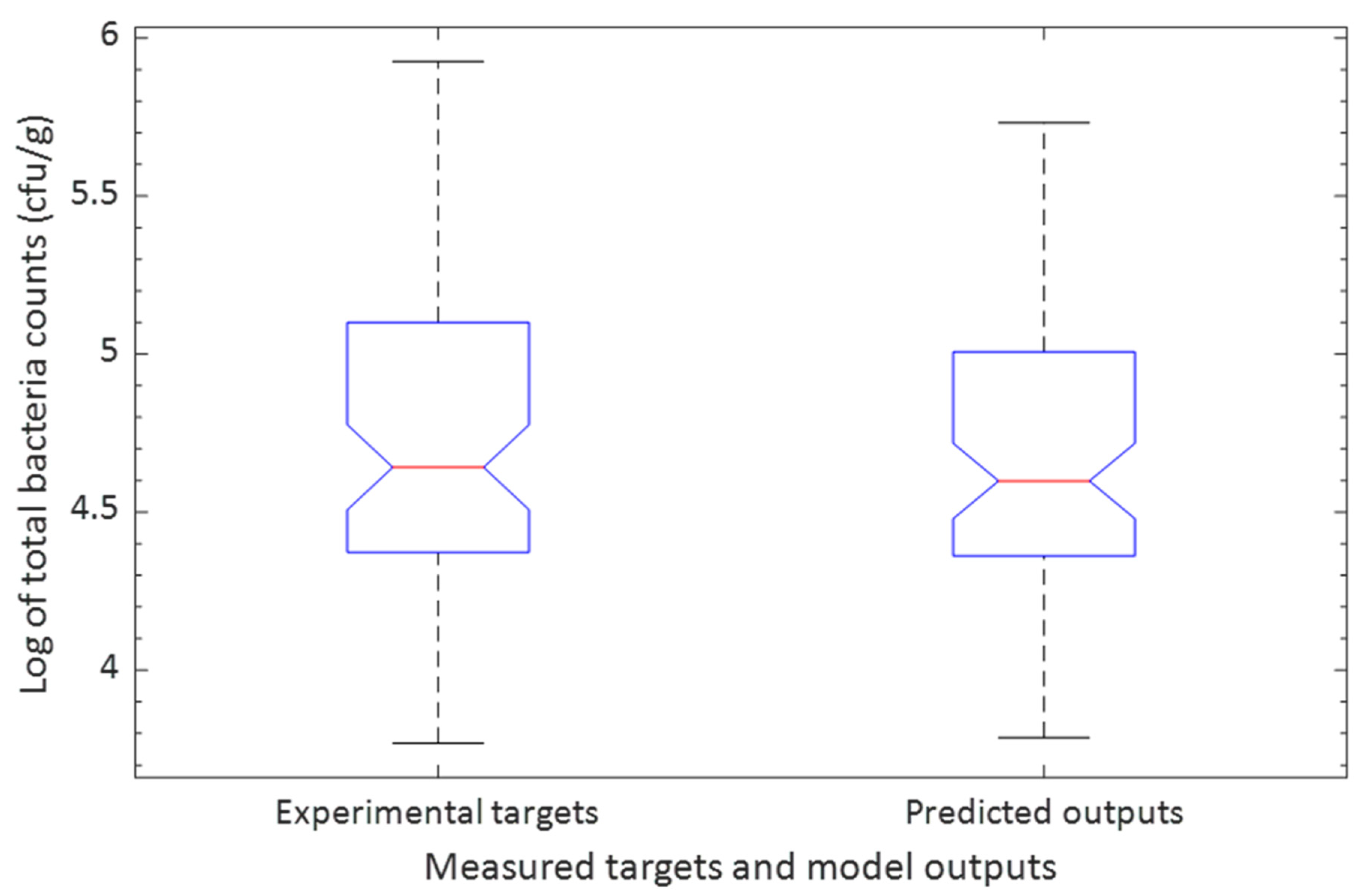
ANOVA Statistics to Confirm Accuracy of the Response Surface Model with Validation Data Set

Table 10. ANOVA table for the validated data set of targets and model outputs.

Statistics Based on Targets and Model Outputs with the Response Surface Model
Source	Sum of Square (SS)	Degree of Freedom (df)	Mean Square (MS)	F Statistic	Prob > F
Columns	0.0966	1	0.0966	0.37	0.5434
Error	36.3955	142	0.2603
Total	37.0521	143

shows the ANOVA table for the targets (experimental determined log of total viable bacteria counts) and the model outputs with the data set used for validation. The degree of freedom of the between and within groups were 1 and 142, respectively. The total degree of freedom was 143. The groups of targets and model outputs as on the table shows that the mean square of the columns and error were 0.966 and 0.2603. The F-statistic was 0.370, whereas the p-value was 0.5434. The p-value (0.5434) was larger than the critical value (0.05) and confirmed that no mean significant difference existed between the targets and predicted model outputs over a 95% confidence level.

In additional the ANOVA plots in Figure 9 shows no outliers and the data set for the targets and model outputs were normally distributed and the means and medians for the targets were 4.7166 cfu/g and 4.6363 cfu/g, whereas for the model outputs they were 4.666 cfu/g and 4.5706 cfu/g, respectively.

4. Conclusions

The study affirmed that cow waste constitutes of adequate biodegradable matter that can result in the generation of substantial biogas during anaerobic digestion in a balloon biodigester. A reliable data acquisition system was designed and built to measure the relevant input parameters for the development of a non-linear response surface model to predict the total viable bacteria counts. All the three predictors (number of days, daily slurry temperature and pH) used in the developed response surface model were primary factors with the number of days, depicted as the most significant contributor by weight of ranking to the log of total viable bacteria counts, whereas the least was the daily slurry temperature. A response surface model was developed to forecast the total viable bacteria counts, whereby the number of days, daily slurry temperature and pH were the predictors. The developed model demonstrated very high accuracy between the experimental targets and the model outputs for both the testing and validation data set. The determination coefficient, root mean square value and p-value between the targets and model outputs for the testing samples were 0.959, 0.197, and 0.602, whereas for the validation samples they were 0.974, 0.341, and 0.543, respectively. Both the p-values and the ANOVA plots showed no significant difference between the targets and models outputs for the testing and validation sampled data set. Furthermore, a 2D multi-contour surface plots was developed to explicitly show the relationship between each predictor with the log of total viable bacteria counts via simulation using the derived response surface model. The results reveal that log of total viable bacteria counts turns to increase with an increase in the daily slurry temperature and the pH. The findings from the study can assist manufacturers and service providers of balloon type biodigesters to understand the variation of multiple inputs parameters with the total viable bacteria counts through the derived 2D multi-contour surface plots simulation. Based on the comparison of the values of the targets and model outputs, we can conclude that the developed non-linear response surface model can be used to predict the total bacteria counts with high accuracy in a balloon digester charged with cow waste.

5. Recommendation for Future Study

A recommendation of a future study should be conducted over the other months of the year (January to June) as ambient weather condition influenced the biogas yield in a balloon digester. A study should also be conducted whereby the balloon digester is charge using the continuous mode. A study should be conducted with co-digestion (between the cow manure and other animal waste (e.g., pig, since the university owned a piggery) as feedstock for the balloon digester.

References

1. Lu, Y.; Khan, Z.A.; Alvarez-Alvarado, M.S.; Zhang, Y.; Huang, Z.; Imran, M. A critical review of sustainable energy policies for the promotion of renewable energy sources. Sustainability 2020, 12, 5078. [Google Scholar] [CrossRef]
2. Abanades, S.; Abbaspour, H.; Ahmadi, A.; Das, B.; Ehyaei, M.A.; Esmaeilion, F.; El Haj Assad, M.; Hajilounezhad, T.; Jamali, D.H.; Hmida, A.; et al. A critical review of biogas production and usage with legislations framework across the globe. Int. J. Environ. Sci. Technol. 2021, 19, 3377–3400. [Google Scholar] [CrossRef]
3. Kemausuor, F.; Adaramola, M.S.; Morken, J. A review of commercial biogas systems and lessons for Africa. Energies 2018, 11, 2984. [Google Scholar] [CrossRef] [Green Version]
4. Ayilara, M.S.; Olanrewaju, O.S.; Babalola, O.O.; Odeyemi, O. Waste management through composting: Challenges and potentials. Sustainability 2020, 12, 4456. [Google Scholar] [CrossRef]
5. Garfí, M.; Martí-Herrero, J.; Garwood, A.; Ferrer, I. Household anaerobic digesters for biogas production in Latin America: A review. Renew. Sustain. Energy Rev. 2016, 60, 599–614. [Google Scholar] [CrossRef] [Green Version]
6. Manyi-Loh, C.E.; Mamphweli, S.N.; Meyer, E.L.; Okoh, A.I.; Makaka, G.; Simon, M. Microbial anaerobic digestion (bio-digesters) as an approach to the decontamination of animal wastes in pollution control and the generation of renewable energy. Int. J. Environ. Res. Public Health 2013, 10, 4390–4417. [Google Scholar] [CrossRef] [Green Version]
7. Wilkie, A.C. Anaerobic digestion of dairy manure: Design and process considerations. In Dairy Manure Management: Treatment, Handling, and Community Relations; Cornell University: Ithaca, NY, USA, 2005; Volume 301, pp. 301–312. [Google Scholar]
8. Mehariya, S.; Patel, A.K.; Obulisamy, P.K.; Punniyakotti, E.; Wong, J.W. Co-digestion of food waste and sewage sludge for methane production: Current status and perspective. Bioresour. Technol. 2018, 265, 519–531. [Google Scholar] [CrossRef]
9. Howarth, R.W.; Santoro, R.; Ingraffea, A. Methane and the greenhouse-gas footprint of natural gas from shale formations. Clim. Chang. 2011, 106, 679–690. [Google Scholar] [CrossRef] [Green Version]
10. Manyi-Loh, C.; Mamphweli, S.; Meyer, E.; Okoh, A. Characterizing Bacteria and Methanogens in a Balloon-Type Digester Fed with Dairy Cattle Manure for Anaerobic Mono-Digestion. Pol. J. Environ. Stud. 2019, 28, 1287–1293. [Google Scholar] [CrossRef]
11. Hagos, K.; Zong, J.; Li, D.; Liu, C.; Lu, X. Anaerobic co-digestion process for biogas production: Progress, challenges and perspectives. Renew. Sustain. Energy Rev. 2017, 76, 1485–1496. [Google Scholar] [CrossRef]
12. Manyi-Loh, C.E.; Mamphweli, S.N.; Meyer, E.L.; Makaka, G.; Simon, M.; Okoh, A.I. An overview of the control of bacterial pathogens in cattle manure. Int. J. Environ. Res. Public Health 2016, 13, 843. [Google Scholar] [CrossRef] [Green Version]
13. Tangwe, S.L.; Simon, M. Evaluation of performance of air source heat pump water heaters using the surface fitting models: 3D mesh plots and 2D multi contour plots simulation. Therm. Sci. Eng. Prog. 2018, 5, 516–523. [Google Scholar] [CrossRef]
14. Dincer, I.; Acar, C. A review on clean energy solutions for better sustainability. Int. J. Energy Res. 2015, 39, 585–606. [Google Scholar] [CrossRef]
15. Morgan, H.M., Jr.; Xie, W.; Liang, J.; Mao, H.; Lei, H.; Ruan, R.; Bu, Q. A techno-economic evaluation of anaerobic biogas producing systems in developing countries. Bioresour. Technol. 2018, 250, 910–921. [Google Scholar] [CrossRef]
16. Pérez, I.; Garfí, M.; Cadena, E.; Ferrer, I. Technical, economic and environmental assessment of household biogas digesters for rural communities. Renew. Energy 2014, 62, 313–318. [Google Scholar] [CrossRef]
17. Hamid, R.G.; Blanchard, R.E. An assessment of biogas as a domestic energy source in rural Kenya: Developing a sustainable business model. Renew. Energy 2018, 121, 368–376. [Google Scholar] [CrossRef] [Green Version]
18. Werner, U.; Stöhr, U.; Hees, N. Biogas Plants in Animal Husbandry; Deutsches Zentrum für Entwicklungstechnologien: Eschborn, Germany, 1989. [Google Scholar]
19. Nzila, C.; Dewulf, J.; Spanjers, H.; Tuigong, D.; Kiriamiti, H.; Van Langenhove, H. Multi criteria sustainability assessment of biogas production in Kenya. Appl. Energy 2012, 93, 496–506. [Google Scholar] [CrossRef]
20. Bakar, N.S.A.; Nasir, N.M.; Lananan, F.; Hamid, S.H.A.; Lam, S.S.; Jusoh, A. Optimization of C/N ratios for nutrient removal in aquaculture system culturing African catfish, (Clarias gariepinus) utilizing Bioflocs Technology. Int. Biodeterior. Biodegrad. 2015, 102, 100–106. [Google Scholar] [CrossRef]
21. Sreela-Or, C.; Plangklang, P.; Imai, T.; Reungsang, A. Co-digestion of food waste and sludge for hydrogen production by anaerobic mixed cultures: Statistical key factors optimization. Int. J. Hydrogen Energy 2011, 36, 14227–14237. [Google Scholar] [CrossRef]
22. Hu, B.; Zhou, W.; Min, M.; Du, Z.; Chen, P.; Ma, X.; Liu, Y.; Lei, H.; Shi, J.; Ruan, R. Development of an effective acidogenically digested swine manure-based algal system for improved wastewater treatment and biofuel and feed production. Appl. Energy 2013, 107, 255–263. [Google Scholar] [CrossRef]
23. Mao, C.; Feng, Y.; Wang, X.; Ren, G. Review on research achievements of biogas from anaerobic digestion. Renew. Sustain. Energy Rev. 2015, 45, 540–555. [Google Scholar] [CrossRef]
24. Koupaie, E.H.; Lin, L.; Lakeh, A.B.; Azizi, A.; Dhar, B.R.; Hafez, H.; Elbeshbishy, E. Performance evaluation and microbial community analysis of mesophilic and thermophilic sludge fermentation processes coupled with thermal hydrolysis. Renew. Sustain. Energy Rev. 2021, 141, 110832. [Google Scholar] [CrossRef]
25. Zhang, T.; Tan, Y.; Zhang, X. Using a hybrid heating system to increase the biogas production of household digesters in cold areas of China: An experimental study. Appl. Therm. Eng. 2016, 103, 1299–1311. [Google Scholar] [CrossRef]
26. Akhbari, A.; Kutty, P.K.; Chuen, O.C.; Ibrahim, S. A study of palm oil mill processing and environmental assessment of palm oil mill effluent treatment. Environ. Eng. Res. 2020, 25, 212–221. [Google Scholar] [CrossRef] [Green Version]
27. Basumatary, S.; Das, S.; Kalita, P.; Goswami, P. Effect of feedstock/water ratio on anaerobic digestion of cattle dung and vegetable waste under mesophilic and thermophilic conditions. Bioresour. Technol. Rep. 2021, 14, 100675. [Google Scholar] [CrossRef]
28. Mahmudul, H.M.; Rasul, M.G.; Akbar, D.; Narayanan, R.; Mofijur, M. A comprehensive review of the recent development and challenges of a solar-assisted biodigester system. Sci. Total Environ. 2021, 753, 141920. [Google Scholar] [CrossRef]
29. Zhao, J.; Hou, T.; Lei, Z.; Shimizu, K.; Zhang, Z. Effect of biogas recirculation strategy on biogas upgrading and process stability of anaerobic digestion of sewage sludge under slightly alkaline condition. Bioresour. Technol. 2020, 308, 123293. [Google Scholar] [CrossRef]
30. Gaballah, E.S.; Abomohra, A.E.F.; Xu, C.; Elsayed, M.; Abdelkader, T.K.; Lin, J.; Yuan, Q. Enhancement of biogas production from rape straw using different co-pretreatment techniques and anaerobic co-digestion with cattle manure. Bioresour. Technol. 2020, 309, 123311. [Google Scholar] [CrossRef]
31. Angenent, L.T.; Sung, S.; Raskin, L. Methanogenic population dynamics during startup of a full-scale anaerobic sequencing batch reactor treating swine waste. Water Res. 2002, 36, 4648–4654. [Google Scholar] [CrossRef]
32. Blessy, M.R.D.P.; Patel, R.D.; Prajapati, P.N.; Agrawal, Y.K. Development of forced degradation and stability indicating studies of drugs—A review. J. Pharm. Anal. 2014, 4, 159–165. [Google Scholar] [CrossRef]
33. Yadav, D.; Barbora, L.; Bora, D.; Mitra, S.; Rangan, L.; Mahanta, P. An assessment of duckweed as a potential lignocellulosic feedstock for biogas production. Int. Biodeterior. Biodegrad. 2017, 119, 253–259. [Google Scholar] [CrossRef]
34. Yu, Q.; Liu, R.; Li, K.; Ma, R. A review of crop straw pretreatment methods for biogas production by anaerobic digestion in China. Renew. Sustain. Energy Rev. 2019, 107, 51–58. [Google Scholar] [CrossRef]
35. Bharathiraja, B.; Sudharsana, T.; Jayamuthunagai, J.; Praveenkumar, R.; Chozhavendhan, S.; Iyyappan, J. Biogas production–A review on composition, fuel properties, feed stock and principles of anaerobic digestion. Renew. Sustain. Energy Rev. 2018, 90, 570–582. [Google Scholar] [CrossRef]
36. Sreekrishnan, T.R.; Kohli, S.; Rana, V. Enhancement of biogas production from solid substrates using different techniques––A review. Bioresour. Technol. 2004, 95, 1–10. [Google Scholar]
37. Gunaseelan, V.N. Anaerobic digestion of biomass for methane production: A review. Biomass Bioenergy 1997, 13, 83–114. [Google Scholar] [CrossRef]
38. Ihara, I.; Yano, K.; Andriamanohiarisoamanana, F.J.; Yoshida, G.; Yuge, T.; Yuge, T.; Tangtaweewipat, S. and Umetsu, K. Field testing of a small-scale anaerobic digester with liquid dairy manure and other organic wastes at an urban dairy farm. J. Mater. Cycles Waste Manag. 2020, 22, 1382–1389. [Google Scholar] [CrossRef]
39. Ferrer, I.; Garfí, M.; Uggetti, E.; Ferrer-Martí, L.; Calderon, A.; Velo, E. Biogas production in low-cost household digesters at the Peruvian Andes. Biomass Bioenergy 2011, 35, 1668–1674. [Google Scholar] [CrossRef]
40. Gupta, P.; Diwan, B. Bacterial exopolysaccharide mediated heavy metal removal: A review on biosynthesis, mechanism and remediation strategies. Biotechnol. Rep. 2017, 13, 58–71. [Google Scholar] [CrossRef]
41. Ziganshina, E.E.; Belostotskiy, D.E.; Shushlyaev, R.V.; Miluykov, V.A.; Vankov, P.Y.; Ziganshin, A.M. Microbial community diversity in anaerobic reactors digesting turkey, chicken, and swine wastes. J. Microbiol. Biotechnol. 2014, 24, 1464–1472. [Google Scholar] [CrossRef]
42. Manyi-Loh, C.E.; Mamphweli, S.N.; Meyer, E.L.; Okoh, A.I.; Makaka, G.; Simon, M. Investigation into the biogas production potential of dairy cattle manure. J. Clean Energy Technol. 2015, 3, 326–331. [Google Scholar] [CrossRef] [Green Version]
43. Fridh, L.; Volpé, S.; Eliasson, L. An accurate and fast method for moisture content determination. Int. J. For. Eng. 2014, 25, 222–228. [Google Scholar] [CrossRef]
44. Bradley, R.L. Moisture and total solids analysis. In Food Analysis; Springer: Boston, MA, USA, 2010; pp. 85–104. [Google Scholar]
45. Van Wychen, S.; Laurens, L.M. Determination of Total Solids and Ash in Algal Biomass: Laboratory Analytical Procedure (LAP) (No. NREL/TP-5100-60956); National Renewable Energy Lab. (NREL): Golden, CO, USA, 2016. [Google Scholar]
46. Sahlström, L. A review of survival of pathogenic bacteria in organic waste used in biogas plants. Bioresour. Technol. 2003, 87, 161–166. [Google Scholar] [CrossRef]
47. Bodhidatta, L.; McDaniel, P.; Sornsakrin, S.; Srijan, A.; Serichantalergs, O.; Mason, C.J. Case-control study of diarrheal disease etiology in a remote rural area in Western Thailand. Am. J. Trop. Med. Hyg. 2010, 83, 1106. [Google Scholar] [CrossRef] [Green Version]
48. Valentine, D.T.; Hahn, B. Essential MATLAB for Engineers and Scientists; Academic Press: Cambridge, MA, USA, 2022. [Google Scholar]
49. Tangwe, S.; Kusakana, K. Using statistical tests to compare the coefficient of performance of air source heat pump water heaters. J. Energy S. Afr. 2022, 33, 40–51. [Google Scholar] [CrossRef]
50. Faggioli, G.; Zendel, O.; Culpepper, J.S.; Ferro, N.; Scholer, F. March. An enhanced evaluation framework for query performance prediction. In European Conference on Information Retrieval; Springer Cham: Cham, Switzerland, 2021; pp. 115–112982. [Google Scholar]
51. Reyes, O.; Morell, C.; Ventura, S. Scalable extensions of the ReliefF algorithm for weighting and selecting features on the multi-label learning context. Neurocomputing 2015, 161, 168–182. [Google Scholar] [CrossRef]
52. Germec, M.; Turhan, I. Predicting the experimental data of the substrate specificity of Aspergillus niger inulinase using mathematical models, estimating kinetic constants in the Michaelis–Menten equation, and sensitivity analysis. Biomass Convers. Biorefinery 2021, 1–12. [Google Scholar] [CrossRef]
53. Tangwe, S.; Kusakana, K. A statistical methodology to compare the performance of residential air source heat pump water heaters. Int. J. Sustain. Energy 2021, 40, 719–738. [Google Scholar]
54. Shirani Faradonbeh, R.; Monjezi, M.; Jahed Armaghani, D. Genetic programing and non-linear multiple regression techniques to predict backbreak in blasting operation. Eng. Comput. 2016, 32, 123–133. [Google Scholar] [CrossRef]
55. Coleman, H.W.; Steele, W.G. Experimentation, Validation, and Uncertainty Analysis for Engineers; John Wiley & Sons: Hoboken, NJ, USA, 2018. [Google Scholar]
56. Horner, I.; Renard, B.; Le Coz, J.; Branger, F.; McMillan, H.K.; Pierrefeu, G. Impact of stage measurement errors on streamflow uncertainty. Water Resour. Res. 2018, 54, 1952–1976. [Google Scholar] [CrossRef] [Green Version]
57. Cioabla, A.E.; Ionel, I.; Dumitrel, G.A.; Popescu, F. Comparative study on factors affecting anaerobic digestion of agricultural vegetal residues. Biotechnol. Biofuels 2012, 5, 1–9. [Google Scholar] [CrossRef] [Green Version]
58. Poux, X.; Aubert, P.M. An agroecological Europe in 2050: Multifunctional Agriculture for Healthy Eating. Findings from the Ten Years for Agroecology (TYFA) Modelling Exercise. Iddri-AScA, Study. 2018. Available online: https://www.iddri.org/sites/default/files/PDF/Publications/Catalogue%20Iddri/Etude/201809-ST0918EN-tyfa.pdf (accessed on 20 August 2022).
59. Zhang, W.; Kong, T.; Xing, W.; Li, R.; Yang, T.; Yao, N.; Lv, D. Links between carbon/nitrogen ratio, synergy and microbial characteristics of long-term semi-continuous anaerobic co-digestion of food waste, cattle manure and corn straw. Bioresource Technol. 2022, 343, 126094. [Google Scholar] [CrossRef] [PubMed]
60. Ibrahim, M.H.; Quaik, S.; Ismail, S.A. An introduction to anaerobic digestion of organic wastes. In Prospects of Organic Waste Management and the Significance of Earthworms; Springer: Cham, Switzerland, 2016; pp. 23–44. [Google Scholar]
61. Babaee, A.; Shayegan, J.; Roshani, A. Anaerobic slurry co-digestion of poultry manure and straw: Effect of organic loading and temperature. J. Environ. Health Sci. Eng. 2013, 11, 15. [Google Scholar] [CrossRef]
62. Rastogi, G.; Ranade, D.R.; Yeole, T.Y.; Patole, M.S.; Shouche, Y.S. Investigation of methanogen population structure in biogas reactor by molecular characterization of methyl-coenzyme M reductase A (mcrA) genes. Bioresour. Technol. 2008, 99, 5317–5326. [Google Scholar] [CrossRef]
63. Choorit, W.; Wisarnwan, P. Effect of temperature on the anaerobic digestion of palm oil mill effluent. Electron. J. Biotechnol. 2007, 10, 376–385. [Google Scholar] [CrossRef]
64. Tangwe, S.L. Demonstration of Residential Air Source Heat Pump Water Heaters Performance in South Africa: Systems Monitoring and Modelling. Doctoral Dissertation, University of Sunderland, Sunderland, UK, 2018. [Google Scholar]
Figure 1. A schematic of a fixed-dome biodigester.
Sustainability 14 13289 g001
Figure 2. Schematic of a floating-drum biodigester.
Sustainability 14 13289 g002
Figure 3. Schematic of the balloon digester charged with cow manure with the installed sensors and data loggers. 1, Bottom slurry temperature sensor; 2, intermediate slurry temperature sensor; 3, biogas temperature sensor; 4, ambient temperature sensor; 5, temperature data logger; 6, biogas analyzer’s transducer; 7, biogas analyzer; 8, gas flow meter; 9, gas flow data logger; 10, weatherproof enclosure; 11, slurry intake; 12, influent chamber; 13, slurry outlet; 14, effluent chamber; 15, reactor chamber; 16, slurry; 17, biogas; 18, balloon digester; 19, control valve; 20, gas pipeline; 21, pump; 22, gas collection chamber; 23, insulation cover; 24, pH data logger; 25, pH transducer.
Sustainability 14 13289 g003
Figure 4. Profiles of ambient temperature, input, and output parameters.
Sustainability 14 13289 g004
Figure 5. Weights ranking of predictors in accordance with the total viable bacteria counts.
Sustainability 14 13289 g005
Figure 6. 2D multi-contour plots of the predictors and modelled output with the non-linear model.
Sustainability 14 13289 g006
Figure 7. Testing data of targets and model outputs based on response surface model.
Sustainability 14 13289 g007
Figure 8. ANOVA plots of targets and model outputs (testing data set).
Sustainability 14 13289 g008
Figure 9. ANOVA plots of targets and model outputs (validation data set).
Sustainability 14 13289 g009