Abstract
Industry 4.0 and its technologies allow advancements in communications, production and management efficiency across several segments. In smart grids, essential parts of smart cities, smart meters act as IoT devices that can gather data and help the management of the sustainable energy matrix, a challenge that is faced worldwide. This work aims to use smart meter data and household features data to seek the most appropriate methods of energy consumption prediction. Using the Cross-Industry Standard Process for Data Mining (CRISP-DM) method, Python Platform, and several prediction methods, prediction experiments were performed with household feature data and past consumption data of over 470 smart meters that gathered data for three years. Support vector machines, random forest regression, and neural networks were the best prediction methods among the ones tested in the sample. The results help utilities (companies that maintain the infrastructure for public services) to offer better contracts to new households and to manage their smart grid infrastructure based on the forecasted demand.
Keywords:
smart meters; forecasting; python; support vector machines; random forest; neural networks 1. Introduction
The term “Industry 4.0” was first introduced at Hannover Fair in 2011. Subsequently, in 2013, the report entitled ‘Industrie 4.0′ developed by a research team recruited by the German government disseminated the term worldwide [1]. The term 4.0 refers to the previous three industrial revolutions. They were represented by advancements in coal and mechanical production in the late 18th century, the advent of electricity and the assembly line in the late 1800s, and finally, the computer and information technology revolution during and after the 1970s [1,2].
The fourth revolution describes many digital technologies and a decentralized production process, based mainly on the use of Radio-frequency identification (RFID), big data, cloud computing, smart sensors, machine learning, robotics, additive manufacturing, artificial intelligence, augmented reality, the Internet of things, material sciences and nanotechnologies [3,4]. These digital technologies enable a systematical deployment of Cyber-Physical Systems (CPS) and bring manufacturing into Industry 4.0 [5]. Industry 4.0’s objective is similar to previous revolutions and aims to increase productivity and enhance mass production using innovative technology [6] as well as advanced planning and control methods [7,8]. Although the “Industry 4.0” term is widely known and used, there are several denominations to describe similar industrial processes in the literature. Analogous concepts have been used with different denominations, such as advanced manufacturing [5], smart industry or factories [9,10], smart manufacturing [11], the industrial Internet of things [5,12], networking manufacturing [9], intelligent manufacturing [13,14], industrial Internet [15], some elements of the national plan carried out by the Chinese government entitled ‘Made in China 2025’ [4], and so on.
Digital technologies, present in Industry 4.0, are heavily used to improve smart cities’ services in terms of quality and efficiency and to help smart cities’ companies by supplying them with information for decision making [16]. A smart city may be described as a place where traditional connections and services are improved using digital technologies to create value for its inhabitants and businesses [17]. There are many opportunities for digital technologies in cities, such as transportation [18], healthcare [19] and buildings [20,21] as well as in energy [22]. Furthermore, the link between energy, sustainability, and smart cities is close because energy efficiency is crucial to increase sustainable urban development [23]. The use of digital technologies to improve traditional power distribution systems is also called a smart grid [24]. As a part of the smart grid, the Advanced Metering Infrastructure (AMI) is an essential component due to its capacity to collect, process, and transfer data through the Internet [24]. Smart meters are a vital component of AMI as a result of their role in the connection between the user and the smart grid [25]. Given the opportunity to apply Industry 4.0 technologies such as big data, the Internet of things, and artificial intelligence using smart meters as a data source, some research is being carried out to predict energy consumption. Such research uses many different approaches, such as clustering [26], conditional kernel density [27], neural networks [28], hierarchical probabilistic forecasts [29], deep learning, and support vector machines [30], among others.
Looking at the reliability, frequency, format, and availability of smart meters’ data [31], added to the smart meters’ importance for both the consumers and the AMI [32], and also taking into account the urgent need to manage resources’ supply and consumption efficiently, we can ask the following question: which is the most appropriate method to make energy consumption predictions based on household features and past energy consumption data? To answer this question, this article aims to test many forecasting methods to indicate an appropriate one to predict energy consumption using household smart meter data. The energy consumption forecast is applied in two different situations. The first situation aims to test different techniques to predict the energy consumption of new homes, for which there are no available previous consumption data. In this case, the energy consumption estimation is predicted based on home features and the appliances that will be available at home; this will be referred to from now on as feature-based prediction. The second one aims to identify an appropriate technique to predict energy consumption using previous consumption data. The approach intends to identify a proper technique to predict energy consumption using time-series data in this case. This will be referred to as past data-based prediction.
This paper is structured as follows: in Section 2, there is a brief review of regression and forecasting methods, Section 3 comprises the methods and materials, and results are shown in Section 4, with further discussion presented in Section 5. Finally, Section 6 offers conclusions and is followed by the References Section.
2. Literature Review
The literature shows that cyber-physical production networks operate automatically and smoothly with artificial intelligence-based decision-making algorithms in a sustainable manner, and Internet of Things-based manufacturing systems function in an automated, robust, and flexible manner [33]. So, we need to understand how IoT devices work along with decision-making algorithms in the context of energy data management.
2.1. Smart Meters
Internet of Things (IoT) technology is a formidable tool for industries, services, and users. This technology improves monitoring, control, customization, and prediction [34]. In the area of utilities (companies that maintain the infrastructure for public services), a successful case of using IoT-connected devices that add value to different stakeholders lies in smart meters [35,36]. These devices constitute an important part of the information technology in smart cities [37], being fundamental parts of smart water and electricity grids [31,38].
Smart meters represent an evolution of traditional, electromechanical meters [31,38]. Electromechanical meters feature manual reading and charging, physical connections, and analog displays. On the other hand, smart meters feature data storage and management, remote bidirectional metering and charging, end-to-end communication, blackout detection, diagnosis systems, In-House Displays (IHD), wireless connections, fast leak detection, and dynamic pricing according to supply and demand [31,38]. These features enable smart meters to become important data sources used in energy/water demand predictions, mainly alongside statistical prediction methods and machine learning.
Smart meters enable consumers to monitor their energy/water consumption in real-time and to produce their own energy, sending the surplus to the smart grid, among other benefits [39,40]. However, beyond the benefits for consumers, smart meters are essential for utilities to handle the increasing share of renewable sources in the energy matrix. It is necessary to adopt sustainable energy sources to mitigate the effects of global warming and climate change [41]. Nevertheless, sustainable sources such as wind, solar, and tidal are naturally generated with instability, and their peak production does not meet peak consumption [42]. Thus, smart meters are needed to gather data in real-time on what is generated, consumed, and stored to prevent and manage shortages [43]. Smart water meters have a similar role, detecting leaks and alerting the utilities as soon as they happen [38].
2.2. Energy Consumption Forecasting Methods
Many planning processes in the energy industry rely on forecasts of unknown future outcomes of relevant system variables. Besides forecasts of electricity prices [44,45], failure predictions for predictive maintenance [46,47], or sales forecasts of products [48,49], forecasts of resource and energy demand [50,51] are essential. This work aims to tackle two occasions on which utilities have to make predictions about energy consumption. The first is when someone moves to a new house and needs to sign an energy supply contract. The utility needs to evaluate how much energy that household is likely to consume, but there is no past consumption data to make a prediction. However, demographic and features data regarding the household may be used alongside some regression methods to predict monthly energy consumption.
Regression methods are supervised learning methods that predict continuous values based on characteristic features describing the behavior of a system. The simplest and most classic example of regression is linear regression. This work tests the accuracy of six regression methods to predict household energy consumption: linear regression, ridge regression, Bayesian ridge regression, support vector regression (scaled and unscaled), and random forest regression.
Ridge regression is commonly used when independent variables are highly correlated and is used in load forecasting as a comparison [52] or in improved versions [53]. Bayesian ridge is a special case of Bayesian linear regression, where the mean of a variable is a linear combination of other variables, and the posterior distribution can be approximated. It was used to reconstruct missing smart meter data [54] and to detect hacker attacks on smart grids [55].
Support vector machines are a class of machine learning methods developed in the United States at the end of the 20th century [56]. These models create vectors forming borders in a hyperspace based on a set of previously classified data to classify new data. The regression version, known as support vector regression (SVR) [57], creates a region in hyperspace where the data points are found. Recent examples of SVR are present in investigating the penetration of photovoltaic sources in microgrids [58] and the classification of household characteristics [59].
Random forest is an ensemble learning method that uses a large number of decision trees based on data characteristics to perform data classification and regression. In random forest regression, a special case of the random forest method, the mean or average prediction of the individual trees is returned [60]. Recent uses of this technique include helping small communities self-manage their electricity grid [61] and investigating energy disaggregation [62].
The other utility concern tackled by this work is when there is past energy consumption data when the utility needs to project future energy consumption for the following months. In this case, time-series forecasting methods can be used. Time-series forecasting methods are a special case of regression methods that try to predict future data values based on past values [63]. Here, we use five time-series forecasting methods: moving average, autoregressive integrated moving-average (ARIMA), exponential smoothing, neural network forecasting, and random forest forecasting. In addition, a naïve forecast (which replicates the last known data for the entire forecast period) is also used for baseline comparison.
Moving average is a common approach for modeling univariate time series, which specifies that the output variable depends linearly on a stochastic term’s current and various past values. ARIMA is an extended approach to moving average, which tries to transform non-stationary time-series into stationary ones and considers their previous values to predict the next ones. It is commonly used in recent studies about electric load prediction [64,65].
Exponential smoothing is a common technique for smoothing the time series using the exponential window function. Exponential functions assign exponentially decreasing weights over time instead of giving equal weights to past observations, as in the case of ARIMA. It is used as a benchmark for comparison in recent smart-meter data studies [27,66].
An artificial neural network, or simply a neural network, is a massively parallel distributed processor made up of simple processing units with a natural propensity for storing experiential knowledge and making it available for use. It resembles the brain in the sense that knowledge is acquired by the network from its environment through a learning process and that interneuron connection strengths, known as synaptic weights, are used to store the acquired knowledge [67]. The long short-term memory (LSTM) approach used in this work is also largely found in other recent studies for commercial building load forecasting, photovoltaic power generation, and residential load forecasting [66,68,69].
Random forest forecasting is a special case of random forest regression, where past data of a time series is given to forecasting future data. It is also commonly found in recent studies about load forecasting [70], peak prediction [71], and fault prediction [72].
3. Materials and Methods
The methodological procedure carried out in this work follows the Shearer (2000) proposal named Cross-Industry Standard Process for Data Mining (CRISP-DM) [73]. This procedure is a widely accepted neutral model, used in the data science literature, utilized, and reviewed in many different cases [74,75,76]. The CRISP-DM activities are organized in six stages: (i) business understanding, (ii) data understanding, (iii) data preparation, (iv) modeling, (v) evaluation, and (vi) deployment. The procedures are displayed following each of the first five steps proposed by CRISP-DM [73], and ways for implementing the sixth step are suggested in the discussion section.
3.1. Business Understanding
Utilities have the mission of generating, supplying, and distributing water, energy, or gas to their consumers. Utility infrastructure is the basis for other sectors of the economy, and utility networks represent the largest structures ever built by humanity [77]. However, the shift from fossil fuel production to renewable energy sources represents an immense challenge in terms of simultaneous management of what is produced, distributed, stored, and consumed [77]. Understanding energy consumption patterns and acting to decrease the infrastructure needed for peak usage will yield savings in the billions of dollars [78,79]. Thus, the need to understand how different residences with distinct characteristics consume natural resources, both in the present and in the future, is clear. Several Industry 4.0 technologies, such as big data, the Internet of things, and artificial intelligence, are used by utilities to manage energy consumption and to understand the consumption patterns of different configurations of households. In this sense, the smart meter is the main enabler of Industry 4.0 technologies for utilities.
In this work, the evaluation of how much energy a household will consume is completed with different regression methods based on the household’s features. The forecasting of how much energy a household will consume in the future was performed by time-series forecasting, using past energy consumed values of that household as a predictor for future values.
3.2. Data Understanding
After understanding the need for utilities, the next step was to find a database of resource consumption recorded by smart meters, which also brought information about the homes in which these meters are installed. The base chosen was the GEM HOUSE project [80], an open database available at the IEEE DataPort [80]. This project gathers the energy consumption of hundreds of German homes between 2018 and 2020. More precisely, the databases “all-users-daily-data.csv” and “household-information.csv” were used. The first database brings daily energy consumption data for each smart meter, with 829,521 rows of data in three columns, as illustrated in Figure 1.
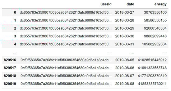
Figure 1.
Sample of “all-users-daily-data.csv” database.
The second base presents several characteristics of 552 households in which the smart meters are installed. These characteristics include data on the area of the residence, the number of people and children, as well as the heating and cooling systems of residences, and the existence and quantity of electric cars, washing machines, televisions, and other appliances. Figure 2 presents a sample of the data from this database, and Figure 3 presents a summary of all the characteristics and types of data.
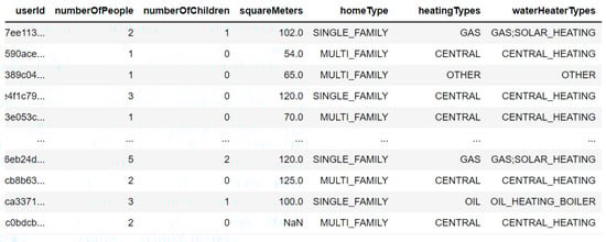
Figure 2.
Sample of “household-information.csv” database.
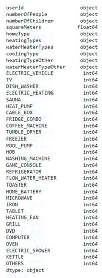
Figure 3.
Features and datatypes of the household’s database.
Figure 4 presents a simplified schematic vision of the information contained in both databases and the link between them.
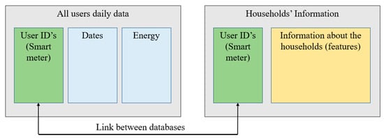
Figure 4.
Schematic vision of the databases.
3.3. Data Preparation
After obtaining the databases, the data were managed using the Jupyter Notebook v. 6.4.5 available in Anaconda Navigator ® v 2.2. Figure 5 presents a schematic vision of the data preparation, followed by a more detailed explanation to ensure reproducibility.
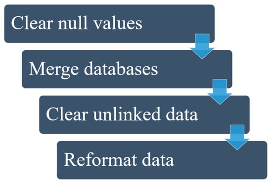
Figure 5.
Data preparation process.
After inspecting a sample of the bases, we explored them to verify the existence of null data. In the database “all-users-daily-data.csv”, there were no null values. In the “household-information.csv” database, the “heatingTypeOther” and “waterHeaterTypeOther” columns were removed because they contain approximately 97% of null values in their structure. Other lines with null values were also removed, totaling a reduction from 552 to 472 lines; that is, 472 unique smart meters. Next, the two databases were merged, using the smart meters identifier (“userId”) as the connection key. Not all meters identified in the “all-users-daily-data.csv” database had household characteristics registered in the other database, so the data from these meters were removed from the merged database.
Some data reformatting had to be performed at the merged base (referred to as the GEM database). First, from the “date” column, an object type data which brings the period of energy consumption, the “dates” column was created with the same information but in the data format for time-series (datetime64[ns]). Then, several columns of data were transformed from “categories” to dummy variables, a format supported by machine learning algorithms. Another necessary transformation was in the reported energy consumption data. In the original format, the reported data is the accumulated amount registered in the smart meter since its installation. This data was transformed into the energy consumed on the recorded day by subtracting the previous value from the current day. As each meter’s first record date did not have the previous day for subtraction, those lines were removed. Thus, a sample of the transformed database is presented in Figure 6 and Figure 7; the whole database has 411,568 rows and 58 columns. Figure 8 shows the list with all data columns and their data type.
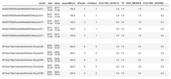
Figure 6.
Sample of the first columns of the transformed database.
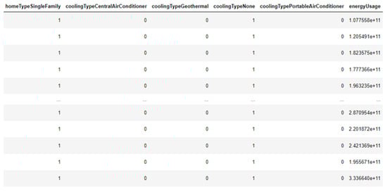
Figure 7.
Sample of the last columns of the transformed database.
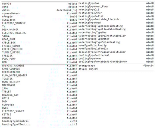
Figure 8.
Data columns and data types of the transformed database.
3.4. Modeling
3.4.1. Feature-Based Prediction
In the feature-based prediction experiment, the objective is to train an algorithm so that, based on the characteristics of a given residence, it can predict the residence’s energy demand. As all data from all smart meters will be used simultaneously, data from smart meters with less than 400 records each were discarded, totaling five smart meters. The energy consumption data were also transformed from a daily to a monthly basis. The database was randomly divided between a training split (80% of the database) and a test split (20% of the database).
For the feature-based experiment using random forest, a random forest regressor was used, imported from the sci-kit learn package. For a feature-based experiment using support vector machines, SVR was used, also imported from sci-kit learn. It is recommended that the values in the database are scaled (normalized) to use the support vector machine algorithm. The algorithm was trained on a scaled and unscaled basis for comparison purposes. The text version of the Jupyter Notebbok with these regression algorithms is in Appendix A.
3.4.2. Past Data-Based Prediction
The objective of the past data-based experiment is to forecast, based on past consumption data provided in a certain period, the energy consumption for a certain period in the future.
For the past data-based experiments, data on the features of the households are not necessary since the forecasting of the consumption of a given smart meter is performed only considering its own past data. Smart meters with less than 901 records were removed to guarantee a robust data history for each smart meter’s forecasting. A looping structure was created for all forecasting algorithms, in which the algorithm trains and forecasts the energy consumption for each smart meter. The division between the training and test sets was performed in temporal terms. The period with the oldest data is the training period, and the most recent period is the testing period. The moving average, ARIMA, and exponential smoothing algorithms were imported from the “statsmodels package”. The LSTM recurrent neural network method, imported from tensorflow, was used for the neural network. The random forest regressor, imported from the “sci-kit learn package”, was used for the random forest forecast. The text version of the Jupyter Notebbok with these regression algorithms is in Appendix B.
3.5. Evaluation
Both in the feature-based and past data-based experiments, the symmetric Mean Absolute Percentage Error (sMAPE) and the Root-Mean-Square Error (RMSE) were used to assess the accuracy of the predicted values. The sMAPE is typically defined according to Equation (1):
where, for every t iteration from the first (t = 1) to the last (t = n) of the series, At is the actual value, and Ft is the predicted value. The “100%” term converts the result to a percentage basis.
The RMSE is defined by Equation (2):
where yj is the actual value and is the predicted value.
For regression experiments, the evaluation is carried out using the mean values of sMAPE and RMSE of the train test split interactions. These values were compiled into a table for comparison. In the case of forecasting experiments, the sMAPE and RMSE values for each smart meter were added to a table and compared among all forecasting methods.
4. Results
4.1. Feature-Based Prediction
The following linear regression methods were used as baselines for comparison with Random Forest Regression and Support Vector Machines Regression: Linear Regression, Bayesian Ridge Linear Regression, and Ridge Linear Regression. The Support Vector Machines without scaling were also used for comparison, resulting in six different regression methods. The sMAPE and RMSE values of the predictions with their corresponding regression method are shown in Table 1.

Table 1.
Error values of the featured-based predictions.
The errors in the estimations indicate that the random forest method presented the best results in both error evaluations (sMAPE and RMSE), followed by the support vector machines method. These findings imply that random forest and support vector machines showed the greatest capacity to predict energy consumption with the data of 476 residences used in this experiment.
Linear regression and ridge linear regression presented very similar results, with error values worse than both random forest and support vector machines. Bayesian ridge linear regression and support vector machines without scaling appeared to be inadequate methods for predicting energy consumption in this experiment since their errors were worse than the baseline of the linear regression method.
4.2. Past Data-Based Prediction
Table 2 summarizes sMAPE and RMSE values for each of the smart meters and forecasting methods.
Table 2.
Error values and correspondent statistical measures for the past data-based predictions.
As a way to evaluate the quality of the forecasting methods, Naïve forecasting was performed. In naïve forecasting, the last record of the training set is predicted in all records of the testing set. It is possible to see that all forecasting methods performed better than the naïve forecasting, which has the highest mean sMAPE, and the highest standard deviation. The same result can be seen if we evaluate the results with the RMSE.
It is possible to notice that the three traditional statistical methods (Moving-average, ARIMA, and Exponential Smoothing) presented very similar results. The three have an average sMAPE between 28.46% and 29.43%, a difference of less than 1% between the means of the three methods. The standard deviation between the three methods also shows a variation of less than 2%, hovering around 15%. The values between the quartiles are also very close. The results obtained with the Random Forest and Neural Network methods in the sample analyzed raised predictions more accurately when compared to the other three methods. Mean, standard deviation and quartile values are each smaller between Neural Network and Random Forest when compared to the Moving Average, ARIMA, and Exponential Smoothing. Based on the results obtained in the smart meter consumption time-series sample, the Neural Network was the more accurate forecasting method.
5. Discussion
The main novelty presented in this work is the comparison of hundreds of different smart meters data to achieve the best prediction methods, among the most standard present in the literature, in two different situations, namely, the feature-based predictions used to predict consumption for new households and the past data-based prediction to foresee long-term infrastructure needs.
5.1. Feature-Based Prediction
The results presented are very important for utilities, as they allow a quick and accurate forecast of energy consumption estimates for new customers. For example, one way to deploy the algorithms of this work (and thus reach the last step of the CRISP-DM method) would be to embed them into an application that quickly calculates values for a real-time pricing (RTP) contract. Using real-time consumption estimates provides the billing flexibility necessary for RTP contracts to be advantageous [81]. Another example of using these consumption prediction algorithms is setting reasonable resource-saving goals in gamification applications [82]. With achievable goals, it is possible that engagement will increase and the goals of rationalizing the use of resources will be achieved. It is important to mention that one of the challenges that utilities will face is how to gather feature data to predict energy consumption, with data disaggregation being one of the main tools to help this data collection without the need for anything external to the smart meters’ energy consumption data [83].
5.2. Past Data-Based Prediction
Predicting future energy use is a key need for utilities. The need to use renewable energy sources to meet sustainability goals [41] is a global reality. Such renewable sources are characterized by variable energy generation over short periods and the non-coincidence between generation peaks and consumption peaks [77]. In this context, it is necessary to use artificial intelligence and data from smart meters to manage energy supply, distribution, and demand.
The application of forecasting algorithms using data from a utility’s entire coverage region allows strategic decisions regarding infrastructure maintenance and expansion, supply diversion, blackout prevention, and storage for peak periods, among others. The daily frequency data presented in this work are more suitable for medium and long-term expansion and maintenance. However, applying the algorithms in smaller interval data, with the respective investigation about micro seasonality, enables utilities to reduce peak consumption and use of energy stored in capacitors, or even in electric cars, to stabilize generation and demand. A business plan for the resource management strategy of a utility that involves the results obtained with this work is also an example of the last step of the CRISP-DM method.
The results are valid for this smaller-scale set of households. Nevertheless, recent results in the literature are aligned with these in the sense that the Neural Networks method is an optimal starting point for developing more complex tools for long-term energy predictions [79,84].
5.3. Data Gathering and Privacy Concerns
Several surveys point to different factors regarding what can facilitate or hinder the acceptance of smart meters. Factors such as perceived usefulness, environmental concerns, and performance expectation are historically the main drivers of consumer acceptance [85,86,87]. Nevertheless, hedonistic motivation and social influence have been gaining strength as acceptance drivers [32]. However, insecurity regarding data protection, data misuse, and hacking can be a factor that drives consumers away from smart meters [83,88,89,90,91]. Gathering consumer data is essential for advancing smart grid management, so actions must be taken to prevent privacy damage and consumer resistance. Some options that apply to smart meters are anonymization technologies and privacy by design, using aggregation, encryption, and steganography techniques [83,92]. Other tools allow the user to adjust the utility’s control over the smart meter in legal terms [93] and in terms of application settings and communications [94,95]. Such options should be considered, so privacy concerns and a lack of control over data do not threaten data gathering.
6. Conclusions
Industry 4.0 and its related technologies are permanently changing the interactions between people and electronic devices. They are helping utilities and governments to better understand and manage all the sources and needs of smart cities, a crucial task in a century where climate change is most felt and scarce resources must be used in the most efficient ways. In this same context, smart meters act as IoT devices, gathering big data that should be used along with artificial intelligence and cloud computing to better manage energy supply and demand. This work sought to identify the more appropriate methods to use the data collected from these smart meters and household features to predict electricity consumption. Several methods were applied to a German dataset using the CRISP-DM framework, and the results were compared.
In theoretical terms, the results of this work offer a comparison between several prediction algorithms. The best prediction methods using feature-based data for the dataset are random forest and support vector machines. Neural networks and random forest showed the best results for past data-based prediction. Starting with these two approaches and developing more complex and comprehensive AI decision-making techniques will help improve the accuracy and robustness of the predictions.
In practical terms, the results of this work contribute to advancements in the management of smart grids by providing more tools and options that facilitate this management. Both the management of new customers, with an easy and quick forecast of energy consumption, and the strategic management of a sustainable future energy supply benefit from the results obtained here. Future challenges are presented in terms of how to gather consumption data without jeopardizing consumers’ privacy. Industries and governments should advance toward privacy by using design tools and smart meter acceptance policies to secure a safe and reliable data source for energy management.
This study provides a comparison between several prediction techniques and shows the best option in the database given. These techniques can be used for companies to predict energy consumption in different scenarios and should be improved by future research linking this data with local economic and meteorological data as well as with correlations between the features and energy consumed.
The 21st century presents immense challenges, including the management of smart cities. We are taking a crucial step towards the smart and sustainable management of natural resources by using the full potential of the data generated by IoT devices combined with machine learning techniques. Such advancements will be decisive for future generations’ quality of life in this century and beyond.
Author Contributions
Conceptualization, J.G., D.C.F., E.M.F. and M.K.; methodology, J.G., D.C.F., and M.K.; software, J.G. and M.K.; validation, D.C.F., E.M.F. and M.K.; formal analysis, J.G.; investigation, J.G.; resources, E.M.F.; data curation, J.G.; writing—original draft preparation, J.G.; writing—review and editing, D.C.F. and M.K.; visualization, J.G.; supervision, E.M.F.; project administration, E.M.F.; funding acquisition, E.M.F. All authors have read and agreed to the published version of the manuscript.
Funding
This research was funded by Coordenação de Aperfeiçoamento de Pessoal de Nível Superior, FAPESC—grant number 2022TR001415, and The Brazilian National Council for Scientific and Technological Development, grant number 200450/2022–0.
Institutional Review Board Statement
Not applicable.
Informed Consent Statement
Not applicable.
Data Availability Statement
The “all-users-daily-data.csv” and “household-information.csv” datasets are available to download at: https://ieee-dataport.org/open-access/gem-house-opendata-german-electricity-consumption-many-households-over-three-years−2018 (accessed on 7 October 2022).
Conflicts of Interest
The authors declare no conflict of interest.
Appendix A. Featured-Based Prediction Algorithm
- (Text version of the Python® Jupyter Notebooks archive)
- #Initial Imports
- import numpy as np
- import pandas as pd
- import matplotlib.pyplot as plt
- from sklearn.metrics import mean_squared_error as rmse
- #load first database
- dataMain = pd.read_csv(‘all-users-daily-data-GEM-House.csv’)
- print(dataMain.shape)
- dataMain.head()
- dataMain
- #checking some details about the database
- df1 = pd.DataFrame(dataMain)
- print (df1.dtypes)
- print (dataMain[‘userId’].nunique())
- print (dataMain.describe())
- earliest = min(dataMain[‘date’])
- print (earliest)
- latest = max(dataMain[‘date’])
- print (latest)
- #looking for null values and duplicates
- print (dataMain.isnull().sum().sum())
- dataMainDup = dataMain.duplicated()
- truesDataMainDup = dataMainDup.sum()
- print (truesDataMainDup)
- #create ‘dates’ column as a time series object
- dataMain[‘dates’] = pd.to_datetime(dataMain[‘date’], format = ‘%Y/%m/%d’)
- #check how the date values are distributed among smart meters
- dataMain[‘date’].value_counts()
- #load second database
- households = pd.read_csv(‘household-information.csv’)
- print(households.shape)
- households.head()
- households
- #checking details about the second database
- df = pd.DataFrame(households)
- print (df.dtypes)
- print (households[‘userId’].nunique())
- print (households[‘numberOfPeople’].nunique())
- print (households[‘numberOfChildren’].nunique())
- print (households[‘homeType’].nunique())
- print (households[‘heatingTypes’].nunique())
- print (households[‘coolingType’].nunique())
- print (households[‘heatingTypeOther’].nunique())
- print (households[‘waterHeaterTypeOther’].nunique())
- households.describe()
- #Checking null values and duplicates(1)
- households.isnull().sum().sum()
- #Checking null values and duplicates(2)
- householdsDup = households.duplicated()
- truesHouseholdsDup = householdsDup.sum()
- truesHouseholdsDup
- #Checking null values and duplicates(3)
- households.columns[households.isna().any()].tolist()
- #Checking null values and duplicates(4)
- print (households[‘numberOfPeople’].isnull().sum().sum())
- print (households[‘numberOfChildren’].isnull().sum().sum())
- print (households[‘squareMeters’].isnull().sum().sum())
- print (households[‘homeType’].isnull().sum().sum())
- print (households[‘heatingTypes’].isnull().sum().sum())
- print (households[‘waterHeaterTypes’].isnull().sum().sum())
- print (households[‘coolingType’].isnull().sum().sum())
- print (households[‘heatingTypeOther’].isnull().sum().sum())
- print (households[‘waterHeaterTypeOther’].isnull().sum().sum())
- households = households.drop(columns = [‘heatingTypeOther’, ‘waterHeaterTypeOther’])
- #Droping lines with null values
- householdsClean = households.dropna()
- householdsClean
- #checking the number of different smart meters
- householdsClean[‘userId’].nunique()
- #list of features of the second database
- features1 = list(householdsClean.columns.values.tolist())
- features1
- #Merging databases
- GEM = dataMain
- GEM = GEM.merge(householdsClean, how = ‘left’, on = ‘userId’)
- #Dropping rows that do not have features corresponding to that smart meter.
- GEM = GEM.dropna()
- GEM
- #Rechecking null values
- GEM.isnull().sum().sum()
- #checking the number of different smart meters
- GEM[‘userId’].nunique()
- #Checking data types.
- df4 = pd.DataFrame(GEM)
- print (df4.dtypes)
- #It is needed to change categorical variables into dummy variables. It is also needed to split columns with more than one
- #response in the same cell, then we have only one information per cell.
- GEM[‘heatingTypes’].value_counts()
- GEM[‘waterHeaterTypes’].value_counts()
- GEM[[‘waterHeaterTypesA’, ‘waterHeaterTypesB’, ‘waterHeaterTypesC’]] = GEM[‘waterHeaterTypes’].str.split(‘;’, −1, expand = True)
- GEM
- #Spliting the information about heating types
- GEM[[‘heatingTypesA’, ‘heatingTypesB’, ‘heatingTypesC’, ‘heatingTypesD’,‘heatingTypesE’]] = GEM[‘heatingTypes’].str.split(‘;’, −1, expand = True)
- #Getting dummies to every heating type column
- GEM[‘heatingTypesE’].value_counts()
- GEM[‘heatingTypesEEletric’] = pd.get_dummies(GEM[‘heatingTypesE’])
- GEM.rename(columns = {‘heatingTypesEEletric’:‘htElectric5’}, inplace = True)
- pd.get_dummies(GEM[‘heatingTypesD’])
- GEM[[‘htElectric4’,‘htGas4’]] = pd.get_dummies(GEM[‘heatingTypesD’])
- pd.get_dummies(GEM[‘heatingTypesC’])
- GEM[[‘htCentral3’,‘htGas3’,‘htPellet3’]] = pd.get_dummies(GEM[‘heatingTypesC’])
- pd.get_dummies(GEM[‘heatingTypesB’])
- GEM[[‘htCentral2’,‘htElectric2’,‘htGas2’,‘htHeat_Pump2’, ‘htOil2’, ‘htPellet2’, ‘htPortable_Electric2’, ‘htWood2’]] = pd.get_dummies(GEM[‘heatingTypesB’])
- pd.get_dummies(GEM[‘heatingTypesA’])
- GEM[[‘htCentral1’,‘htElectric1’,‘htGas1’,‘htHeat_Pump1’, ‘htOil1’, ‘htOther1’, ‘htPellet1’, ‘htPortable_Electric1’, ‘htWood1’]] = pd.get_dummies(GEM[‘heatingTypesA’])
- #Getting one column to each heating type
- GEM[‘heatingTypeCentral’] = GEM[‘htCentral3’] + GEM[‘htCentral2’] + GEM[‘htCentral1’]
- GEM[‘heatingTypeElectric’] = GEM[‘htElectric5’] + GEM[‘htElectric4’] + GEM[‘htElectric2’] + GEM[‘htElectric1’]
- GEM[‘heatingTypeGas’] = GEM[‘htGas4’] + GEM[‘htGas3’] + GEM[‘htGas2’] + GEM[‘htGas1’]
- GEM[‘heatingTypeHeat_Pump’] = GEM[‘htHeat_Pump2’] + GEM[‘htHeat_Pump1’]
- GEM[‘heatingTypeOil’] = GEM[‘htOil2’] + GEM[‘htOil1’]
- GEM[‘heatingTypeOther’] = GEM[‘htOther1’]
- GEM[‘heatingTypePellet’] = GEM[‘htPellet3’] + GEM[‘htPellet2’] + GEM[‘htPellet1’]
- GEM[‘heatingTypePortable_Electric’] = GEM[‘htPortable_Electric2’] + GEM[‘htPortable_Electric1’]
- GEM[‘heatingTypeWood’] = GEM[‘htWood2’] + GEM[‘htWood1’]
- GEM
- #Dropping the columns created to allocate data in the middle of the process
- GEM = GEM.drop([‘heatingTypesA’,
- ‘heatingTypesB’, ‘heatingTypesC’, ‘heatingTypesD’, ‘heatingTypesE’, ‘htElectric5’, ‘htElectric4’, ‘htGas4’, ‘htCentral3’, ‘htGas3’, ‘htPellet3’, ‘htCentral2’, ‘htElectric2’, ‘htGas2’, ‘htHeat_Pump2’, ‘htOil2’, ‘htPellet2’, ‘htPortable_Electric2’, ‘htWood2’, ‘htCentral1’, ‘htElectric1’, ‘htGas1’, ‘htHeat_Pump1’, ‘htOil1’, ‘htOther1’, ‘htPellet1’, ‘htPortable_Electric1’, ‘htWood1’], axis = 1)
- list(GEM.columns.values.tolist())
- #Spliting and getting dummy variables for water heating types
- GEM[‘waterHeaterTypes’].value_counts()
- GEM[[‘waterHeaterTypesA’, ‘waterHeaterTypesB’, ‘waterHeaterTypesC’]] = GEM[‘waterHeaterTypes’].str.split(‘;’, −1, expand = True)
- #Checking the categories
- pd.get_dummies(GEM[‘waterHeaterTypesA’])
- pd.get_dummies(GEM[‘waterHeaterTypesB’])
- pd.get_dummies(GEM[‘waterHeaterTypesC’])
- #Getting dummies
- GEM[[‘wtCentralHeating1’,‘wtFlowWaterHeating1’,‘wtGas1’,‘wtOilHeatingBoiler1’, ‘wtOther1’,
- ‘wtSolarHeating1’]] = pd.get_dummies(GEM[‘waterHeaterTypesA’])
- GEM[[‘wtCentralHeating2’,‘wtFlowWaterHeating2’,‘wtGas2’,‘wtOilHeatingBoiler2’, ‘wtSolarHeating2’]] = pd.get_dummies(GEM[‘waterHeaterTypesB’])
- GEM[[‘wtFlowWaterHeating3’,‘wtSolarHeating3’]] = pd.get_dummies(GEM[‘waterHeaterTypesC’])
- #Summing the commom categories into one column
- GEM[‘waterHeatingTypeCentralHeating’] = GEM[‘wtCentralHeating1’] + GEM[‘wtCentralHeating2’]
- GEM[‘waterHeatingTypeFlowWaterHeating’] = GEM[‘wtFlowWaterHeating1’] + GEM[‘wtFlowWaterHeating2’] + GEM[‘wtFlowWaterHeating3’]
- GEM[‘waterHeatingTypeGas’] = GEM[‘wtGas1’] + GEM[‘wtGas2’]
- GEM[‘waterHeatingTypeOilHeatingBoiler’] = GEM[‘wtOilHeatingBoiler1’] + GEM[‘wtOilHeatingBoiler2’]
- GEM[‘waterHeatingTypeOther’] = GEM[‘wtOther1’]
- GEM[‘waterHeatingTypeSolarHeating’] = GEM[‘wtSolarHeating1’] + GEM[‘wtSolarHeating2’] + GEM[‘wtSolarHeating3’]
- #Dropping intermediate columns
- GEM = GEM.drop([‘waterHeaterTypesA’, ‘waterHeaterTypesB’, ‘waterHeaterTypesC’,‘wtCentralHeating1’, ‘wtFlowWaterHeating1’, ‘wtGas1’, ‘wtOilHeatingBoiler1’, ‘wtOther1’, ‘wtSolarHeating1’, ‘wtCentralHeating2’, ‘wtFlowWaterHeating2’, ‘wtGas2’, ‘wtOilHeatingBoiler2’, ‘wtSolarHeating2’, ‘wtFlowWaterHeating3’, ‘wtSolarHeating3’],axis = 1)
- GEM
- #Dropping the two original categorical columns
- GEM = GEM.drop([‘heatingTypes’, ‘waterHeaterTypes’],axis = 1)
- GEM
- #The next variables do not have more than one info per cell
- #Getting dummies for home type
- pd.get_dummies(GEM[‘homeType’])
- GEM[[‘homeTypeMultiFamily’,‘homeTypeSingleFamily’]] = pd.get_dummies(GEM[‘homeType’])
- #Getting dummies for cooling type
- pd.get_dummies(GEM[‘coolingType’])
- GEM[[‘coolingTypeCentralAirConditioner’,‘coolingTypeGeothermal’, ‘coolingTypeNone’,‘coolingTypePortableAirConditioner’]] = pd.get_dummies(GEM[‘coolingType’])
- #Dropping the original columns
- GEM = GEM.drop([‘homeType’, ‘coolingType’],axis = 1)
- #Sorting rows by user id and date
- GEM = GEM.sort_values([‘userId’, ‘date’])
- #Creating a new variable, subtracting the energy value from the previous column, so we have the energy consumed, instead of the
- #energy accumulated
- GEM[‘energyUsage’] = GEM[‘energy’].diff()
- GEM
- GEM.isnull().sum().sum()
- #We need to delete the first row of every smart meter, because we do not have the previous value to subtract
- GEM[‘num_in_group’] = GEM.groupby(‘userId’).cumcount()
- GEM = GEM[GEM[‘num_in_group’] > 0]
- GEM
- GEM[‘numberOfPeople’].value_counts()
- GEM[‘numberOfChildren’].value_counts()
- #We need to transform ‘number of people’ and ‘number of children’ into integers.
- #First we deal with the ‘8 + ’ and ‘7 + ’ issue.
- GEM[‘nPeople’] = [8 if a == ‘8 + ’ else a for a in GEM[‘numberOfPeople’]]
- GEM[‘nChildren’] = [7 if a == ‘7 + ’ else a for a in GEM[‘numberOfChildren’]]
- #Then we change the data type
- GEM[‘nPeople’] = GEM[‘nPeople’].astype(int)
- GEM[‘nChildren’] = GEM[‘nChildren’].astype(int)
- #Finally we delete the original columns, including the original energy column
- GEM = GEM.drop([‘energy’,
- ‘numberOfPeople’,
- ‘numberOfChildren’,‘num_in_group’],axis = 1)
- GEM
- #Shifting the columns’ order to have the energy as the last column
- cols = GEM.columns.tolist()
- cols
- cols = [‘userId’, ‘date’, ‘dates’, ‘squareMeters’, ‘nPeople’, ‘nChildren’, ELECTRIC_VEHICLE’, ‘TV’, ‘DISH_WASHER’, ‘ELECTRIC_HEATING’, ‘SAUNA’, ‘HEAT_PUMP’, ‘CABLE_BOX’, ‘FRIDGE_COMBO’, ‘COFFEE_MACHINE’, ‘TUMBLE_DRYER’, ‘FREEZER’, ‘POOL_PUMP’, ‘HOB’, ‘WASHING_MACHINE’, ‘GAME_CONSOLE’, ‘REFRIGERATOR’, ‘FLOW_WATER_HEATER’, ‘TOASTER’, ‘HOME_BATTERY’, ‘MICROWAVE’, ‘IRON’, ‘TABLET’, ‘HEATING_FAN’, ‘GRILL’, ‘DVD’, ‘COMPUTER’, ‘OVEN’, ‘ELECTRIC_SHOWER’, ‘KETTLE’, ‘OTHERS’, ‘heatingTypeCentral’, ‘heatingTypeElectric’, ‘heatingTypeGas’, ‘heatingTypeHeat_Pump’, ‘heatingTypeOil’, ‘heatingTypeOther’, ‘heatingTypePellet’, ‘heatingTypePortable_Electric’, ‘heatingTypeWood’, ‘waterHeatingTypeCentralHeating’, ‘waterHeatingTypeFlowWaterHeating’, ‘waterHeatingTypeGas’, ‘waterHeatingTypeOilHeatingBoiler’, ‘waterHeatingTypeOther’, ‘waterHeatingTypeSolarHeating’, ‘homeTypeMultiFamily’, ‘homeTypeSingleFamily’, ‘coolingTypeCentralAirConditioner’, ‘coolingTypeGeothermal’, ‘coolingTypeNone’, ‘coolingTypePortableAirConditioner’, ‘energyUsage’]
- GEM = GEM[cols]
- GEM
- #Now all the data types are correct
- #pd.set_option(‘display.max_rows’, None)
- df1 = pd.DataFrame(GEM)
- print (df1.dtypes)
- # Define the function to calculate the sMAPE
- #import numpy as np
- def smape(a, f):
- return 1/len(a) * np.sum(200 * np.abs(f-a) / (np.abs(a) + np.abs(f)))
- #Sorting the rows by date, to set the dates as index
- GEM = GEM.sort_values(by = [‘dates’, ‘userId’])
- #indexing
- GEM = GEM.set_index(GEM[‘dates’])
- GEM = GEM.sort_index()
- GEM
- #Checking how many rows we have for each smart meter
- pd.set_option(‘display.max_rows’, 10)
- GEM[‘userId’].value_counts(sort = False)
- #Creating a new database, dropping smart meters with less than 400 rows
- GEM2 = GEM[GEM.groupby(‘userId’).userId.transform(‘count’) > 399].copy()
- GEM2[‘userId’].value_counts(sort = False)
- #We now have 467 smart meters
- #Creating the Features Matrix and separating it from the energy consumption
- GEM_Features = GEM2
- GEM_Features = GEM_Features.drop([‘date’, ‘dates’,‘energyUsage’ ], axis = 1)
- GEM_Features = GEM_Features.groupby(‘userId’).first().reset_index()
- GEM_Features
- #Creating the energy consumption matrix and summing by month
- GEM_Energy = GEM2
- GEM_Energy = GEM_Energy.drop([ ‘date’, ‘squareMeters’, ‘nPeople’, ‘nChildren’, ‘ELECTRIC_VEHICLE’, ‘TV’, ‘DISH_WASHER’,
- ‘ELECTRIC_HEATING’, ‘SAUNA’, ‘HEAT_PUMP’, ‘CABLE_BOX’, ‘FRIDGE_COMBO’, ‘COFFEE_MACHINE’,
- ‘TUMBLE_DRYER’, ‘FREEZER’, ‘POOL_PUMP’, ‘HOB’, ‘WASHING_MACHINE’, ‘GAME_CONSOLE’, ‘REFRIGERATOR’,
- ‘FLOW_WATER_HEATER’, ‘TOASTER’, ‘HOME_BATTERY’, ‘MICROWAVE’, ‘IRON’, ‘TABLET’, ‘HEATING_FAN’,
- ‘GRILL’, ‘DVD’, ‘COMPUTER’, ‘OVEN’, ‘ELECTRIC_SHOWER’, ‘KETTLE’, ‘OTHERS’, ‘heatingTypeCentral’,
- ‘heatingTypeElectric’, ‘heatingTypeGas’, ‘heatingTypeHeat_Pump’, ‘heatingTypeOil’,
- ‘heatingTypeOther’, ‘heatingTypePellet’, ‘heatingTypePortable_Electric’, ‘heatingTypeWood’,
- ‘waterHeatingTypeCentralHeating’, ‘waterHeatingTypeFlowWaterHeating’, ‘waterHeatingTypeGas’,
- ‘waterHeatingTypeOilHeatingBoiler’, ‘waterHeatingTypeOther’, ‘waterHeatingTypeSolarHeating’,
- ‘homeTypeMultiFamily’, ‘homeTypeSingleFamily’, ‘coolingTypeCentralAirConditioner’,
- ‘coolingTypeGeothermal’, ‘coolingTypeNone’, ‘coolingTypePortableAirConditioner’], axis = 1)
- GEM_Energy = GEM_Energy.groupby([‘userId’, GEM_Energy[‘dates’].dt.to_period(‘M’)]).sum()
- GEM_Energy = GEM_Energy.reset_index(level = ‘userId’)
- GEM_Energy = GEM_Energy.reset_index()
- GEM_Energy
- #Merging GEM_Energy and GEM_Features, setting energyUsage as last column
- GEM_C = GEM_Energy
- GEM_C = GEM_C.merge(GEM_Features, how = ‘left’, on = ‘userId’)
- GEM_C
- cols = [‘userId’, ‘dates’, ‘squareMeters’, ‘nPeople’, ‘nChildren’, ELECTRIC_VEHICLE’, ‘TV’, ‘DISH_WASHER’, ‘ELECTRIC_HEATING’, ‘SAUNA’, ‘HEAT_PUMP’, ‘CABLE_BOX’, ‘FRIDGE_COMBO’, ‘COFFEE_MACHINE’, ‘TUMBLE_DRYER’, ‘FREEZER’, ‘POOL_PUMP’, ‘HOB’, ‘WASHING_MACHINE’, ‘GAME_CONSOLE’, ‘REFRIGERATOR’, ‘FLOW_WATER_HEATER’, ‘TOASTER’, ‘HOME_BATTERY’, ‘MICROWAVE’, ‘IRON’, ‘TABLET’, ‘HEATING_FAN’, ‘GRILL’, ‘DVD’, ‘COMPUTER’, ‘OVEN’, ‘ELECTRIC_SHOWER’, ‘KETTLE’, ‘OTHERS’, ‘heatingTypeCentral’, ‘heatingTypeElectric’, ‘heatingTypeGas’, ‘heatingTypeHeat_Pump’, ‘heatingTypeOil’, ‘heatingTypeOther’, ‘heatingTypePellet’, ‘heatingTypePortable_Electric’, ‘heatingTypeWood’, ‘waterHeatingTypeCentralHeating’, ‘waterHeatingTypeFlowWaterHeating’, ‘waterHeatingTypeGas’, ‘waterHeatingTypeOilHeatingBoiler’, ‘waterHeatingTypeOther’, ‘waterHeatingTypeSolarHeating’, ‘homeTypeMultiFamily’, ‘homeTypeSingleFamily’, ‘coolingTypeCentralAirConditioner’, ‘coolingTypeGeothermal’, ‘coolingTypeNone’, ‘coolingTypePortableAirConditioner’, ‘energyUsage’]
- GEM_C = GEM_C[cols]
- GEM_C
- #Drop ID’s and dates
- GEM_C = GEM_C.drop([‘userId’, ‘dates’ ], axis = 1)
- GEM_C
- #Imports for classification
- import os
- import random
- import itertools
- import numpy as np
- import pandas as pd
- import matplotlib.pyplot as plt
- from sklearn.manifold import TSNE
- from sklearn.preprocessing import StandardScaler
- from sklearn.model_selection import train_test_split
- from sklearn.metrics import accuracy_score, confusion_matrix, classification_report
- #Train-Test Split
- y = GEM_C[‘energyUsage’]
- X_train, X_test, y_train, y_test = train_test_split(GEM_C, y, random_state = 1, test_size = 0.2)
- y_train.shape
- X_train.shape
- X_train
- X_train = X_train.drop([‘energyUsage’], axis = 1)
- X_test = X_test.drop([‘energyUsage’], axis = 1)
- X_test
- y_test.shape
- X_test.shape
- #Random Forest Regressor
- from sklearn.ensemble import RandomForestRegressor
- forest = RandomForestRegressor(1000)
- forest.fit(X_train, y_train)
- #xfit = np.linspace(0, 10, 1000)
- #y_pred = forest.predict(X_test)
- # Use the forest’s predict method on the test data
- predictions = forest.predict(X_test)
- # Calculate the absolute errors
- error = smape(y_test, predictions)
- error2 = rmse(y_test, predictions, squared = False)
- # Print out the errors
- print(‘Smape:’, round(np.mean(error), 2), ‘.’)
- print(‘RMSE:’, round(np.mean(error2), 2), ‘.’)
- SummaryTable = pd.DataFrame(columns = [‘Method’, ‘sMAPE’, ‘RMSE’])
- SummaryTable = SummaryTable.append({‘Method’: ‘Random Forest’, ‘sMAPE’: error, ‘RMSE’: error2},ignore_index = True)
- print(SummaryTable)
- #Support Vector Machines Regression (without Standard Scaling)
- from sklearn.svm import SVR
- SVMregressor = SVR(kernel = ‘rbf’)
- SVMregressor.fit(X_train, y_train)
- y_pred = SVMregressor.predict(X_test)
- errorSVM = smape(y_test, y_pred)
- error2SVM = rmse(y_test, y_pred, squared = False)
- print(‘Smape:’, round(np.mean(errorSVM), 2), ‘.’)
- print(‘RMSE:’, round(np.mean(error2SVM), 2), ‘.’)
- SummaryTable = SummaryTable.append({‘Method’: ‘SVM w/o Scaling’, ‘sMAPE’: errorSVM, ‘RMSE’: error2SVM},ignore_index = True)
- print(SummaryTable)
- #Support Vector Machines Regression (with Standard Scaling)
- from sklearn.preprocessing import StandardScaler
- sc_X = StandardScaler()
- sc_y = StandardScaler()
- X = sc_X.fit_transform(X_train)
- y_train2 = y_train.array.reshape(−1, 1)
- y = sc_y.fit_transform(y_train2)
- X2 = sc_X.fit_transform(X_test)
- regressor = SVR(kernel = ‘rbf’)
- regressor.fit(X, y)
- y_pred = regressor.predict(X2)
- y_pred = sc_y.inverse_transform(y_pred)
- errorSVM = smape(y_test, y_pred)
- error2SVM = rmse(y_test, y_pred, squared = False)
- print(‘Smape:’, round(np.mean(errorSVM), 2), ‘.’)
- print(‘RMSE:’, round(np.mean(error2SVM), 2), ‘.’)
- SummaryTable = SummaryTable.append({‘Method’: ‘SVM with Scaling’, ‘sMAPE’: errorSVM, ‘RMSE’: error2SVM},ignore_index = True)
- print(SummaryTable)
- #Linear Regression (Baseline)
- from sklearn import linear_model, metrics
- reg = linear_model.LinearRegression()
- reg.fit(X_train, y_train)
- y_pred2 = reg.predict(X_test)
- errorSVM = smape(y_test, y_pred2)
- error2SVM = rmse(y_test, y_pred2, squared = False)
- print(‘Smape:’, round(np.mean(errorSVM), 2), ‘.’)
- print(‘RMSE:’, round(np.mean(error2SVM), 2), ‘.’)
- SummaryTable = SummaryTable.append({‘Method’: ‘Linear Regression’, ‘sMAPE’: errorSVM, ‘RMSE’: error2SVM},ignore_index = True)
- print(SummaryTable)
- #Bayesian Ridge Linear Regression
- from sklearn.linear_model import BayesianRidge
- BaRi = BayesianRidge()
- BaRi.fit(X_train, y_train)
- y_pred3 = BaRi.predict(X_test)
- errorSVM = smape(y_test, y_pred3)
- error2SVM = rmse(y_test, y_pred3, squared = False)
- print(‘Smape:’, round(np.mean(errorSVM), 2), ‘.’)
- print(‘RMSE:’, round(np.mean(error2SVM), 2), ‘.’)
- SummaryTable = SummaryTable.append({‘Method’: ‘Bayesian Ridge’, ‘sMAPE’: errorSVM, ‘RMSE’: error2SVM},ignore_index = True)
- print(SummaryTable)
- #Ridge Linear Regression
- from sklearn.linear_model import Ridge
- Ridgemodel = Ridge(alpha = 225)
- Ridgemodel.fit(X_train, y_train)
- y_pred4= Ridgemodel.predict(X_test)
- errorSVM = smape(y_test, y_pred4)
- error2SVM = rmse(y_test, y_pred4, squared = False)
- print(‘Smape:’, round(np.mean(errorSVM), 2), ‘.’)
- print(‘RMSE:’, round(np.mean(error2SVM), 2), ‘.’)
- SummaryTable = SummaryTable.append({‘Method’: ‘Ridge Linear Regression’, ‘sMAPE’: errorSVM, ‘RMSE’: error2SVM},ignore_index = True)
- print(SummaryTable)
Appendix B. Past Data-Based Prediction Algorithm
- (Text version of the Python® Jupyter Notebooks archive)
- #Initial Imports
- import numpy as np
- import pandas as pd
- import matplotlib.pyplot as plt
- fifrom sklearn.metrics import mean_squared_error as rmse
- #load first database
- dataMain = pd.read_csv(‘all-users-daily-data-GEM-House.csv’)
- print(dataMain.shape)
- dataMain.head()
- dataMain
- #checking some details about the database
- df1 = pd.DataFrame(dataMain)
- print (df1.dtypes)
- print (dataMain[‘userId’].nunique())
- print (dataMain.describe())
- earliest = min(dataMain[‘date’])
- print (earliest)
- latest = max(dataMain[‘date’])
- print (latest)
- #looking for null values and duplicates
- print (dataMain.isnull().sum().sum())
- dataMainDup = dataMain.duplicated()
- truesDataMainDup = dataMainDup.sum()
- print (truesDataMainDup)
- #create ‘dates’ column as a time series object
- dataMain[‘dates’] = pd.to_datetime(dataMain[‘date’], format = ‘%Y/%m/%d’)
- #check how the date values are distributed among smart meters
- dataMain[‘date’].value_counts()
- #load second database
- households = pd.read_csv(‘household-information.csv’)
- print(households.shape)
- households.head()
- households
- #checking detais about the second database
- df = pd.DataFrame(households)
- print (df.dtypes)
- print (households[‘userId’].nunique())
- print (households[‘numberOfPeople’].nunique())
- print (households[‘numberOfChildren’].nunique())
- print (households[‘homeType’].nunique())
- print (households[‘heatingTypes’].nunique())
- print (households[‘coolingType’].nunique())
- print (households[‘heatingTypeOther’].nunique())
- print (households[‘waterHeaterTypeOther’].nunique())
- households.describe()
- #Checking null values and duplicates(1)
- households.isnull().sum().sum()
- #Checking null values and duplicates(2)
- householdsDup = households.duplicated()
- truesHouseholdsDup = householdsDup.sum()
- truesHouseholdsDup
- #Checking null values and duplicates(3)
- households.columns[households.isna().any()].tolist()
- #Checking null values and duplicates(4)
- print (households[‘numberOfPeople’].isnull().sum().sum())
- print (households[‘numberOfChildren’].isnull().sum().sum())
- print (households[‘squareMeters’].isnull().sum().sum())
- print (households[‘homeType’].isnull().sum().sum())
- print (households[‘heatingTypes’].isnull().sum().sum())
- print (households[‘waterHeaterTypes’].isnull().sum().sum())
- print (households[‘coolingType’].isnull().sum().sum())
- print (households[‘heatingTypeOther’].isnull().sum().sum())
- print (households[‘waterHeaterTypeOther’].isnull().sum().sum())
- households = households.drop(columns = [‘heatingTypeOther’, ‘waterHeaterTypeOther’])
- #Droping lines with null values
- householdsClean = households.dropna()
- householdsClean
- #checking the number of different smart meters
- householdsClean[‘userId’].nunique()
- #list of features of the second database
- features1 = list(householdsClean.columns.values.tolist())
- features1
- #Merging databases
- GEM = dataMain
- GEM = GEM.merge(householdsClean, how = ‘left’, on = ‘userId’)
- #Dropping rows that do not have features corresponding to that smart meter.
- GEM = GEM.dropna()
- GEM
- #Rechecking null values
- GEM.isnull().sum().sum()
- #checking the number of different smart meters
- GEM[‘userId’].nunique()
- #Checking data types.
- df4 = pd.DataFrame(GEM)
- print (df4.dtypes)
- #It is needed to change categorical variables into dummy variables. It is also needed to split columns with more than one
- #response in the same cell, then we have only one information per cell.
- GEM[‘heatingTypes’].value_counts()
- GEM[‘waterHeaterTypes’].value_counts()
- GEM[[‘waterHeaterTypesA’, ‘waterHeaterTypesB’, ‘waterHeaterTypesC’]] = GEM[‘waterHeaterTypes’].str.split(‘;’, −1, expand = True)
- GEM
- #Spliting the information about heating types
- GEM[[‘heatingTypesA’, ‘heatingTypesB’, ‘heatingTypesC’, ‘heatingTypesD’,‘heatingTypesE’]] = GEM[‘heatingTypes’].str.split(‘;’, −1, expand = True)
- #Getting dummies to every heating type column
- GEM[‘heatingTypesE’].value_counts()
- GEM[‘heatingTypesEEletric’] = pd.get_dummies(GEM[‘heatingTypesE’])
- GEM.rename(columns = {‘heatingTypesEEletric’:‘htElectric5’}, inplace = True)
- pd.get_dummies(GEM[‘heatingTypesD’])
- GEM[[‘htElectric4’,‘htGas4’]] = pd.get_dummies(GEM[‘heatingTypesD’])
- pd.get_dummies(GEM[‘heatingTypesC’])
- GEM[[‘htCentral3’,‘htGas3’,‘htPellet3’]] = pd.get_dummies(GEM[‘heatingTypesC’])
- pd.get_dummies(GEM[‘heatingTypesB’])
- GEM[[‘htCentral2’,‘htElectric2’,‘htGas2’,‘htHeat_Pump2’, ‘htOil2’, ‘htPellet2’, ‘htPortable_Electric2’, ‘htWood2’]] = pd.get_dummies(GEM[‘heatingTypesB’])
- pd.get_dummies(GEM[‘heatingTypesA’])
- GEM[[‘htCentral1’,‘htElectric1’,‘htGas1’,‘htHeat_Pump1’, ‘htOil1’, ‘htOther1’, ‘htPellet1’, ‘htPortable_Electric1’, ‘htWood1’]] = pd.get_dummies(GEM[‘heatingTypesA’])
- #Getting one column to each heating type
- GEM[‘heatingTypeCentral’] = GEM[‘htCentral3’] + GEM[‘htCentral2’] + GEM[‘htCentral1’]
- GEM[‘heatingTypeElectric’] = GEM[‘htElectric5’] + GEM[‘htElectric4’] + GEM[‘htElectric2’] + GEM[‘htElectric1’]
- GEM[‘heatingTypeGas’] = GEM[‘htGas4’] + GEM[‘htGas3’] + GEM[‘htGas2’] + GEM[‘htGas1’]
- GEM[‘heatingTypeHeat_Pump’] = GEM[‘htHeat_Pump2’] + GEM[‘htHeat_Pump1’]
- GEM[‘heatingTypeOil’] = GEM[‘htOil2’] + GEM[‘htOil1’]
- GEM[‘heatingTypeOther’] = GEM[‘htOther1’]
- GEM[‘heatingTypePellet’] = GEM[‘htPellet3’] + GEM[‘htPellet2’] + GEM[‘htPellet1’]
- GEM[‘heatingTypePortable_Electric’] = GEM[‘htPortable_Electric2’] + GEM[‘htPortable_Electric1’]
- GEM[‘heatingTypeWood’] = GEM[‘htWood2’] + GEM[‘htWood1’]
- GEM
- #Dropping the columns created to allocate data in the middle of the process
- GEM = GEM.drop([‘heatingTypesA’,
- ‘heatingTypesB’, ‘heatingTypesC’, ‘heatingTypesD’, ‘heatingTypesE’, ‘htElectric5’, ‘htElectric4’, ‘htGas4’, ‘htCentral3’, ‘htGas3’, ‘htPellet3’, ‘htCentral2’, ‘htElectric2’, ‘htGas2’, ‘htHeat_Pump2’, ‘htOil2’, ‘htPellet2’, ‘htPortable_Electric2’, ‘htWood2’, ‘htCentral1’, ‘htElectric1’, ‘htGas1’, ‘htHeat_Pump1’, ‘htOil1’, ‘htOther1’, ‘htPellet1’, ‘htPortable_Electric1’, ‘htWood1’],axis = 1)
- list(GEM.columns.values.tolist())
- #Spliting and getting dummy variables for water heating types
- GEM[‘waterHeaterTypes’].value_counts()
- GEM[[‘waterHeaterTypesA’, ‘waterHeaterTypesB’, ‘waterHeaterTypesC’]] = GEM[‘waterHeaterTypes’].str.split(‘;’, −1, expand = True)
- #Checking the categories
- pd.get_dummies(GEM[‘waterHeaterTypesA’])
- pd.get_dummies(GEM[‘waterHeaterTypesB’])
- pd.get_dummies(GEM[‘waterHeaterTypesC’])
- #Getting dummies
- GEM[[‘wtCentralHeating1’,‘wtFlowWaterHeating1’,‘wtGas1’,‘wtOilHeatingBoiler1’, ‘wtOther1’,
- ‘wtSolarHeating1’]] = pd.get_dummies(GEM[‘waterHeaterTypesA’])
- GEM[[‘wtCentralHeating2’,‘wtFlowWaterHeating2’,‘wtGas2’,‘wtOilHeatingBoiler2’, ‘wtSolarHeating2’]] = pd.get_dummies(GEM[‘waterHeaterTypesB’])
- GEM[[‘wtFlowWaterHeating3’,‘wtSolarHeating3’]] = pd.get_dummies(GEM[‘waterHeaterTypesC’])
- #Summing the commom categories into one column
- GEM[‘waterHeatingTypeCentralHeating’] = GEM[‘wtCentralHeating1’] + GEM[‘wtCentralHeating2’]
- GEM[‘waterHeatingTypeFlowWaterHeating’] = GEM[‘wtFlowWaterHeating1’] + GEM[‘wtFlowWaterHeating2’] + GEM[‘wtFlowWaterHeating3’]
- GEM[‘waterHeatingTypeGas’] = GEM[‘wtGas1’] + GEM[‘wtGas2’]
- GEM[‘waterHeatingTypeOilHeatingBoiler’] = GEM[‘wtOilHeatingBoiler1’] + GEM[‘wtOilHeatingBoiler2’]
- GEM[‘waterHeatingTypeOther’] = GEM[‘wtOther1’]
- GEM[‘waterHeatingTypeSolarHeating’] = GEM[‘wtSolarHeating1’] + GEM[‘wtSolarHeating2’] + GEM[‘wtSolarHeating3’]
- #Dropping intermediate columns
- GEM = GEM.drop([‘waterHeaterTypesA’, ‘waterHeaterTypesB’, ‘waterHeaterTypesC’,‘wtCentralHeating1’, ‘wtFlowWaterHeating1’, ‘wtGas1’, ‘wtOilHeatingBoiler1’, ‘wtOther1’, ‘wtSolarHeating1’, ‘wtCentralHeating2’, ‘wtFlowWaterHeating2’, ‘wtGas2’, ‘wtOilHeatingBoiler2’, ‘wtSolarHeating2’, ‘wtFlowWaterHeating3’, ‘wtSolarHeating3’],axis = 1)
- GEM
- #Dropping the two original categorical columns
- GEM = GEM.drop([‘heatingTypes’, ‘waterHeaterTypes’],axis = 1)
- GEM
- #The next variables do not have more than one info per cell
- #Getting dummies for home type
- pd.get_dummies(GEM[‘homeType’])
- GEM[[‘homeTypeMultiFamily’,‘homeTypeSingleFamily’]] = pd.get_dummies(GEM[‘homeType’])
- #Getting dummies for cooling type
- pd.get_dummies(GEM[‘coolingType’])
- GEM[[‘coolingTypeCentralAirConditioner’,‘coolingTypeGeothermal’, ‘coolingTypeNone’,‘coolingTypePortableAirConditioner’]] = pd.get_dummies(GEM[‘coolingType’])
- #Dropping the original columns
- GEM = GEM.drop([‘homeType’, ‘coolingType’],axis = 1)
- #Sorting rows by user id and date
- GEM = GEM.sort_values([‘userId’, ‘date’])
- #Creating a new variable, subtracting the energy value from the previous column, so we have the energy consumed, instead of the
- #energy accumulated
- GEM[‘energyUsage’] = GEM[‘energy’].diff()
- GEM
- GEM.isnull().sum().sum()
- #We need to delete the first row of every smart meter, because we do not have the previous value to subtract
- GEM[‘num_in_group’] = GEM.groupby(‘userId’).cumcount()
- GEM = GEM[GEM[‘num_in_group’] > 0]
- GEM
- GEM[‘numberOfPeople’].value_counts()
- GEM[‘numberOfChildren’].value_counts()
- #We need to transform ‘number of people’ and ‘number of children’ into integers.
- #First we deal with the ‘8 + ’ and ‘7 + ’ issue.
- GEM[‘nPeople’] = [8 if a == ‘8 + ’ else a for a in GEM[‘numberOfPeople’]]
- GEM[‘nChildren’] = [7 if a == ‘7 + ’ else a for a in GEM[‘numberOfChildren’]]
- #Then we change the data type
- GEM[‘nPeople’] = GEM[‘nPeople’].astype(int)
- GEM[‘nChildren’] = GEM[‘nChildren’].astype(int)
- #Finally we delete the original columns, including the original energy column
- GEM = GEM.drop([‘energy’,
- ‘numberOfPeople’,
- ‘numberOfChildren’,‘num_in_group’],axis = 1)
- GEM
- #Shifting the columns’ order to have the energy as the last column
- cols = GEM.columns.tolist()
- cols
- cols = [‘userId’, ‘date’, ‘dates’, ‘squareMeters’, ‘nPeople’, ‘nChildren’, ELECTRIC_VEHICLE’, ‘TV’, ‘DISH_WASHER’, ‘ELECTRIC_HEATING’, ‘SAUNA’, ‘HEAT_PUMP’, ‘CABLE_BOX’, ‘FRIDGE_COMBO’, ‘COFFEE_MACHINE’, ‘TUMBLE_DRYER’, ‘FREEZER’, ‘POOL_PUMP’, ‘HOB’, ‘WASHING_MACHINE’, ‘GAME_CONSOLE’, ‘REFRIGERATOR’, ‘FLOW_WATER_HEATER’, ‘TOASTER’, ‘HOME_BATTERY’, ‘MICROWAVE’, ‘IRON’, ‘TABLET’, ‘HEATING_FAN’, ‘GRILL’, ‘DVD’, ‘COMPUTER’, ‘OVEN’, ‘ELECTRIC_SHOWER’, ‘KETTLE’, ‘OTHERS’, ‘heatingTypeCentral’, ‘heatingTypeElectric’, ‘heatingTypeGas’, ‘heatingTypeHeat_Pump’, ‘heatingTypeOil’, ‘heatingTypeOther’, ‘heatingTypePellet’, ‘heatingTypePortable_Electric’, ‘heatingTypeWood’, ‘waterHeatingTypeCentralHeating’, ‘waterHeatingTypeFlowWaterHeating’, ‘waterHeatingTypeGas’, ‘waterHeatingTypeOilHeatingBoiler’, ‘waterHeatingTypeOther’, ‘waterHeatingTypeSolarHeating’, ‘homeTypeMultiFamily’, ‘homeTypeSingleFamily’, ‘coolingTypeCentralAirConditioner’, ‘coolingTypeGeothermal’, ‘coolingTypeNone’, ‘coolingTypePortableAirConditioner’, ‘energyUsage’]
- GEM = GEM[cols]
- GEM
- #Now all the data types are correct
- #pd.set_option(‘display.max_rows’, None)
- df1 = pd.DataFrame(GEM)
- print (df1.dtypes)
- # Define the function to calculate the sMAPE
- #import numpy as np
- def smape(a, f):
- return 1/len(a) * np.sum(200 * np.abs(f-a) / (np.abs(a) + np.abs(f)))
- #importing tools to forecast
- import os
- import statsmodels as sm
- from statsmodels.tsa.api import ExponentialSmoothing, SimpleExpSmoothing, Holt
- from statsmodels.tsa.arima.model import ARIMA
- %matplotlib inline
- #Sorting the rows by date, to set the dates as index
- GEM = GEM.sort_values(by = [‘dates’, ‘userId’])
- #indexing
- GEM = GEM.set_index(GEM[‘dates’])
- GEM = GEM.sort_index()
- GEM
- #Checking how many rows we have for each smart meter
- pd.set_option(‘display.max_rows’, 10)
- GEM[‘userId’].value_counts(sort = False)
- #Creating a new database, dropping smart meters with less than 900 rows
- GEM2 = GEM[GEM.groupby(‘userId’).userId.transform(‘count’) > 900].copy()
- GEM2[‘userId’].value_counts(sort = False)
- #We now have 277 smart meters
- #Splitting the dataset into two slices (test and train) to feed in the forecast models
- GEM_test2 = GEM2[‘2020–05−01’:‘2020–10−31’]
- GEM_train2 = GEM2[‘2017–11−02’:‘2020–04−30’]
- #Checking if the two slices have the same number of unique smart meters
- GEM_test2[‘userId’].nunique()
- GEM_train2[‘userId’].nunique()
- #Creating a smart meters’ list to be used in forecast loops
- uniqueIds = list(set(GEM_train2[‘userId’]))
- nIds = len(uniqueIds)
- nIds
- #Naive forecasts (baseline)
- #creating the error’s recording table
- smapesNaiveTable = pd.DataFrame(columns = [‘Id’, ‘sMAPE_nf’])
- RMSENaiveTable = pd.DataFrame(columns = [‘Id’, ‘RMSE_nf’])
- #Setting loop
- for x in uniqueIds:
- #filtering for every smart meter
- GEM_train2x = GEM_train2.loc[GEM_train2[‘userId’] == x]
- GEM_test2x = GEM_test2.loc[GEM_test2[‘userId’] == x]
- #setting the number of forecasts
- n_train = len(GEM_train2x)
- n_test = len(GEM_test2x)
- #Setting the frequency of the data
- GEM_train2x.index = pd.DatetimeIndex(GEM_train2x.index.values,
- freq = GEM_train2x.index.inferred_freq)
- #applying the forecast model
- y_hat_naive = GEM_test2x.copy()
- y_hat_naive[‘naive_forecast’] = GEM_train2x[‘energyUsage’][n_train−1]
- #getting the error value
- sMAPE_nf= smape(GEM_test2x[‘energyUsage’].values,y_hat_naive[‘naive_forecast’].values)
- RMSE_nf= rmse(GEM_test2x[‘energyUsage’].values,y_hat_naive[‘naive_forecast’].values, squared = False)
- #recording the error value
- smapesNaiveTable = smapesNaiveTable.append({‘Id’: x, ‘sMAPE_nf’: sMAPE_nf},ignore_index = True)
- RMSENaiveTable = RMSENaiveTable.append({‘Id’: x, ‘RMSE_nf’: RMSE_nf},ignore_index = True)
- print(smapesNaiveTable)
- #IdMean = GEMx[‘energyUsage’].mean()
- smapesNaiveTable.describe()
- RMSENaiveTable.describe()
- RMSENaiveTable
- #Moving Average forecasts
- #creating the error’s recording table
- smapesTable = pd.DataFrame(columns = [‘Id’, ‘sMAPE_ma’])
- RMSETable = pd.DataFrame(columns = [‘Id’, ‘RMSE_ma’])
- #Setting loop
- for x in uniqueIds:
- #filtering for every smart meter
- GEM_train2x = GEM_train2.loc[GEM_train2[‘userId’] == x]
- GEM_test2x = GEM_test2.loc[GEM_test2[‘userId’] == x]
- #setting the number of forecasts
- n_train = len(GEM_train2x)
- n_test = len(GEM_test2x)
- #Setting the frequency of the data
- GEM_train2x.index = pd.DatetimeIndex(GEM_train2x.index.values,
- freq = GEM_train2x.index.inferred_freq)
- #applying the forecast model
- y_hat_ma = GEM_test2x.copy()
- model = ARIMA(GEM_train2x[‘energyUsage’], order = (1, 0, 0))
- model_fit = model.fit()
- y_hat_ma = model_fit.forecast(n_test)
- #getting the error value
- sMAPE_ma= smape(GEM_test2x[‘energyUsage’].values,y_hat_ma.values)
- RMSE_ma = rmse(GEM_test2x[‘energyUsage’].values,y_hat_ma.values, squared = False)
- #recording the error value
- smapesTable = smapesTable.append({‘Id’: x, ‘sMAPE_ma’: sMAPE_ma},ignore_index = True)
- RMSETable = RMSETable.append({‘Id’: x, ‘RMSE_ma’: RMSE_ma},ignore_index = True)
- print(smapesTable)
- #IdMean = GEMx[‘energyUsage’].mean()
- #Getting the mean error value
- MeanSmapeMA = smapesTable[‘sMAPE_ma’].mean()
- MeanSmapeMA
- MeanRMSEMA= RMSETable[‘RMSE_ma’].mean()
- MeanRMSEMA
- RMSETable.describe()
- #Arima forecasts
- #creating the error’s recording table
- smapesTable1 = pd.DataFrame(columns = [‘Id’, ‘sMAPE_arima’])
- RMSETable1 = pd.DataFrame(columns = [‘Id’, ‘RMSE_arima’])
- #Setting loop
- for x in uniqueIds:
- #filtering for every smart meter
- GEM_train2x = GEM_train2.loc[GEM_train2[‘userId’] == x]
- GEM_test2x = GEM_test2.loc[GEM_test2[‘userId’] == x]
- #setting the number of forecasts
- n_train = len(GEM_train2x)
- n_test = len(GEM_test2x)
- #Setting the frequency of the data
- GEM_train2x.index = pd.DatetimeIndex(GEM_train2x.index.values,
- freq = GEM_train2x.index.inferred_freq)
- #applying the forecast model
- model = ARIMA(GEM_train2x[‘energyUsage’], order = (1,1,1))
- model_fit = model.fit()
- y_hat_arima = model_fit.forecast(n_test)
- #getting the error value
- sMAPE_arima= smape(GEM_test2x[‘energyUsage’].values,y_hat_arima.values)
- RMSE_arima= rmse(GEM_test2x[‘energyUsage’].values,y_hat_arima.values, squared = False)
- #recording the error value
- smapesTable1 = smapesTable1.append({‘Id’: x, ‘sMAPE_arima’: sMAPE_arima},ignore_index = True)
- RMSETable1 = RMSETable1.append({‘Id’: x, ‘RMSE_arima’: RMSE_arima},ignore_index = True)
- print(smapesTable1)
- #Getting the mean error value
- MeanSmapeARIMA = smapesTable1[‘sMAPE_arima’].mean()
- MeanSmapeARIMA
- RMSETable1.describe()
- #Exponential Smoothing Forecasts -> Auto parameter optimization
- #creating the error’s recording table
- smapesTable2 = pd.DataFrame(columns = [‘Id’, ‘sMAPE_ES’])
- RMSETable2 = pd.DataFrame(columns = [‘Id’, ‘RMSE_ES’])
- #Setting loop
- for x in uniqueIds:
- #filtering for every smart meter
- GEM_train2x = GEM_train2.loc[GEM_train2[‘userId’] == x]
- GEM_test2x = GEM_test2.loc[GEM_test2[‘userId’] == x]
- #setting the number of forecasts
- n_train = len(GEM_train2x)
- n_test = len(GEM_test2x)
- #Setting the frequency of the data
- GEM_train2x.index = pd.DatetimeIndex(GEM_train2x.index.values,
- freq = GEM_train2x.index.inferred_freq)
- #applying the forecast model
- fit3 = SimpleExpSmoothing(GEM_train2x[‘energyUsage’], initialization_method = “estimated”).fit()
- fcast3 = fit3.forecast(n_test).rename(r”$\alpha = %s$” % fit3.model.params[“smoothing_level”])
- #getting the error value
- sMAPE_es= smape(GEM_test2x[‘energyUsage’].values,fcast3.values)
- RMSE_es= rmse(GEM_test2x[‘energyUsage’].values,fcast3.values, squared = False)
- #recording the error value
- smapesTable2 = smapesTable2.append({‘Id’: x, ‘sMAPE_ES’: sMAPE_es},ignore_index = True)
- RMSETable2 = RMSETable2.append({‘Id’: x, ‘RMSE_ES’: RMSE_es},ignore_index = True)
- print(smapesTable2)
- #Getting the mean error value
- MeanSmapeSES = smapesTable2[‘sMAPE_ES’].mean()
- MeanSmapeSES
- #Import tools for Neural Network forecasts
- import tensorflow as tf
- from tensorflow.keras.models import Sequential
- from tensorflow.keras.layers import Dense
- from tensorflow.keras.layers import LSTM
- from sklearn.preprocessing import MinMaxScaler
- from sklearn.metrics import mean_squared_error
- #Neural Network with LSTM Recurrent Neural Networks forecasts
- #creating the error’s recording table
- smapesTable3 = pd.DataFrame(columns = [‘Id’, ‘sMAPE_NN’])
- RMSETable3 = pd.DataFrame(columns = [‘Id’, ‘RMSE_NN’])
- #Setting a specific database to this forecast
- GEMNN= pd.DataFrame()
- GEMNN[[‘userId’, ‘Energy’]] = GEM2[[‘userId’, ‘energyUsage’]]
- scaler = MinMaxScaler(feature_range = (0, 1))
- #GEMNN = scaler.fit_transform(GEMNN)
- sm = 1
- #Setting loop
- for x in uniqueIds:
- #filtering for every smart meter
- GEMNNx = GEMNN.loc[GEMNN[‘userId’] == x]
- GEMNNx = GEMNNx.drop([‘userId’],axis = 1)
- GEMNNx = GEMNNx.reset_index(drop = True)
- GEMNNx = scaler.fit_transform(GEMNNx)
- #setting the number of forecasts
- train_size = int(len(GEMNNx) * 0.80)
- test_size = len(GEMNNx) - train_size
- train, test = GEMNNx [0:train_size], GEMNNx[train_size:len(GEMNNx)]
- #print(len(train), len(test))
- #print(train [1:2], test [1:2])
- #Building the datasets that will feed the model
- dataX, dataY = [], []
- for i in range(len(train)−2):
- a = train[i:i + 1]
- b = train[i + 1:i + 2]
- dataX.append(a)
- dataY.append(b)
- trainX, trainY = np.array(dataX), np.array(dataY)
- trainY3d = np.vstack(trainY)
- trainY2d = np.ravel(trainY3d)
- #print(trainY2d)
- dataU, dataV = [], []
- for i in range(len(test)−2):
- c = test[i:i + 1]
- d = test[i + 1:i + 2]
- dataU.append(c)
- dataV.append(d)
- testX, testY = np.array(dataU), np.array(dataV)
- testY3d = np.vstack(testY)
- testY2d = np.ravel(testY3d)
- #print(testY2d)
- #Reshape the datasets to feed the model
- trainX = np.reshape(trainX, (trainX.shape[0], 1, trainX.shape[1]))
- testX = np.reshape(testX, (testX.shape[0], 1, testX.shape[1]))
- #applying the forecast model
- look_back = 1
- model = Sequential()
- model.add(LSTM(4, input_shape = (1, look_back)))
- model.add(Dense(1))
- model.compile(loss = ‘mean_squared_error’, optimizer = ‘adam’)
- model.fit(trainX, trainY, epochs = 150, batch_size = 1, verbose = 2)#epochs = 100 is the real deal
- # make predictions
- trainPredict = model.predict(trainX)
- testPredict = model.predict(testX)
- # invert predictions
- trainPredict = scaler.inverse_transform(trainPredict)
- trainY2d = scaler.inverse_transform([trainY2d]) #have to fix it, originally it was trainY, but the array dimension was wrong
- testPredict = scaler.inverse_transform(testPredict)
- testY2d = scaler.inverse_transform([testY2d]) #have to fix it, originally it was testY, but the array dimension was wrong
- # calculate root mean squared error
- #trainScore = np.sqrt(mean_squared_error(trainY[0], trainPredict[:,0]))
- #print(‘Train Score: %.2f RMSE’ % (trainScore))
- #testScore = np.sqrt(mean_squared_error(testY[0], testPredict[:,0]))
- #print(‘Test Score: %.2f RMSE’ % (testScore))
- #getting the error value
- sMAPE_nn= smape(testY2d[0], testPredict[:,0])
- RMSE_nn= rmse(testY2d[0], testPredict[:,0], squared = False)
- #recording the error value
- smapesTable3 = smapesTable3.append({‘Id’: x, ‘sMAPE_NN’: sMAPE_nn},ignore_index = True)
- RMSETable3 = RMSETable3.append({‘Id’: x, ‘RMSE_NN’: RMSE_nn},ignore_index = True)
- print(‘Smart Meter number:’, sm)
- sm = sm + 1
- print(smapesTable3)
- #Getting the mean error value
- MeanSmapeNN = smapesTable3[‘sMAPE_NN’].mean()
- print(MeanSmapeNN)
- print(smapesTable3)
- #Getting the mean error value
- MeanSmapeNN = smapesTable3[‘sMAPE_NN’].mean()
- MeanSmapeNN
- #Random Forest Imports and function definitions
- from numpy import asarray
- from pandas import DataFrame
- from pandas import concat
- from sklearn.metrics import mean_absolute_error
- from sklearn.ensemble import RandomForestRegressor
- # transform a time series dataset into a supervised learning dataset
- def series_to_supervised(data, n_in = 1, n_out = 1, dropnan = True):
- n_vars = 1 if type(data) is list else data.shape[1]
- df = DataFrame(data)
- cols = list()
- # input sequence (t-n, ... t−1)
- for i in range(n_in, 0, −1):
- cols.append(df.shift(i))
- # forecast sequence (t, t + 1, ... t + n)
- for i in range(0, n_out):
- cols.append(df.shift(-i))
- # put it all together
- agg = concat(cols, axis = 1)
- # drop rows with NaN values
- if dropnan:
- agg.dropna(inplace = True)
- return agg.values
- # split a univariate dataset into train/test sets
- def train_test_split(data, n_test):
- return data[:-n_test, :], data[-n_test:, :]
- # fit an random forest model and make a one step prediction
- def random_forest_forecast(train, testX):
- # transform list into array
- train = asarray(train)
- # split into input and output columns
- trainX, trainy = train[:, :−1], train[:, −1]
- # fit model
- model = RandomForestRegressor(n_estimators = 1000)
- model.fit(trainX, trainy)
- # make a one-step prediction
- yhat = model.predict([testX])
- return yhat[0]
- # walk-forward validation for univariate data
- def walk_forward_validation(data, n_test):
- predictions = list()
- # split dataset
- train, test = train_test_split(data, n_test)
- # seed history with training dataset
- history = [x for x in train]
- # step over each time-step in the test set
- for i in range(len(test)):
- # split test row into input and output columns
- testX, testy = test[i, :−1], test[i, −1]
- # fit model on history and make a prediction
- yhat = random_forest_forecast(history, testX)
- # store forecast in list of predictions
- predictions.append(yhat)
- # add actual observation to history for the next loop
- history.append(test[i])
- # summarize progress
- #print(‘ > expected = %.1f, predicted = %.1f’ % (testy, yhat))
- # estimate prediction error
- error = smape(test[:, −1], predictions)
- error2 = rmse(test[:, −1], predictions, squared = False)
- return error, error2, test[:, −1], predictions
- #Random Forest forecasts
- #creating the error’s recording table
- smapesTable4 = pd.DataFrame(columns = [‘Id’, ‘sMAPE_RF’])
- RMSETable4 = pd.DataFrame(columns = [‘Id’, ‘RMSE_RF’])
- #Setting a specific database to this forecast
- GEMRF= pd.DataFrame()
- GEMRF[[‘userId’, ‘Energy’]] = GEM2[[‘userId’, ‘energyUsage’]]
- sm = 1
- #Setting loop
- for x in uniqueIds:
- #filtering for every smart meter
- GEMRFx = GEMRF.loc[GEMRF[‘userId’] == x]
- GEMRFx = GEMRFx.drop([‘userId’],axis = 1)
- GEMRFx = GEMRFx.reset_index(drop = True)
- values =GEMRFx.values
- # transform the time series data into supervised learning
- data = series_to_supervised(values, n_in = 10)#n_in = 6 originally
- # evaluate and getting the error value
- smape_rf,rmse_rf, y, yhat = walk_forward_validation(data, 12)
- #recording the error value
- smapesTable4 = smapesTable4.append({‘Id’: x, ‘sMAPE_RF’: smape_rf},ignore_index = True)
- RMSETable4 = RMSETable4.append({‘Id’: x, ‘RMSE_RF’: rmse_rf},ignore_index = True)
- print(‘Smart Meter number:’, sm)
- sm = sm + 1
- print(smapesTable4)
- #Getting the mean error value
- MeanSmapeRF = smapesTable4[‘sMAPE_RF’].mean()
- MeanSmapeRF
- RMSETable4.describe()
- #Naive forecast to be a baseline and compare with the other methods.
- smapesTable = smapesTable.merge(smapesTable1, how = ‘left’, on = ‘Id’)
- smapesTable = smapesTable.merge(smapesTable2, how = ‘left’, on = ‘Id’)
- smapesTable = smapesTable.merge(smapesTable3, how = ‘left’, on = ‘Id’)
- smapesTable = smapesTable.merge(smapesTable4, how = ‘left’, on = ‘Id’)
- smapesTable = smapesTable.merge(smapesNaiveTable, how = ‘left’, on = ‘Id’)
- smapesTable
- smapesTable.describe()
- RMSETable = RMSETable.merge(RMSETable1, how = ‘left’, on = ‘Id’)
- RMSETable = RMSETable.merge(RMSETable2, how = ‘left’, on = ‘Id’)
- RMSETable = RMSETable.merge(RMSETable3, how = ‘left’, on = ‘Id’)
- RMSETable = RMSETable.merge(RMSETable4, how = ‘left’, on = ‘Id’)
- RMSETable = RMSETable.merge(RMSENaiveTable, how = ‘left’, on = ‘Id’)
- RMSETable
- RMSETable.describe()
References
- Kagermann, H.; Helbig, J.; Hellinger, A.; Wahlster, W. Recommendations for Implementing the Strategic Initiative INDUSTRIE 4.0: Securing the Future of German Manufacturing Industry; Final Report of the Industrie 4.0 Working Group: Berlin, Germany, 2013. [Google Scholar]
- Schwab, K. The Fourth Industrial Revolution; Currency: New York, NY, USA, 2017. [Google Scholar]
- Fettermann, D.C.; Cavalcante, C.G.S.; de Almeida, T.D.; Tortorella, G.L. How Does Industry 4.0 Contribute to Operations Management? J. Ind. Prod. Eng. 2018, 35, 255–268. [Google Scholar] [CrossRef]
- Li, L. China’s Manufacturing Locus in 2025: With a Comparison of “Made-in-China 2025” and “Industry 4.0”. Technol. Forecast. Soc. Chang. 2018, 135, 66–74. [Google Scholar] [CrossRef]
- Lee, J.; Bagheri, B.; Kao, H.-A. A Cyber-Physical Systems Architecture for Industry 4.0-Based Manufacturing Systems. Manuf. Lett. 2015, 3, 18–23. [Google Scholar] [CrossRef]
- Demir, K.A.; Döven, G.; Sezen, B. Industry 5.0 and Human-Robot Co-Working. Procedia. Comput. Sci. 2019, 158, 688–695. [Google Scholar] [CrossRef]
- Leusin, M.; Frazzon, E.; Uriona Maldonado, M.; Kück, M.; Freitag, M. Solving the Job-Shop Scheduling Problem in the Industry 4.0 Era. Technologies 2018, 6, 107. [Google Scholar] [CrossRef]
- Frazzon, E.M.; Kück, M.; Freitag, M. Data-Driven Production Control for Complex and Dynamic Manufacturing Systems. CIRP Annals 2018, 67, 515–518. [Google Scholar] [CrossRef]
- Davis, J.; Edgar, T.; Porter, J.; Bernaden, J.; Sarli, M. Smart Manufacturing, Manufacturing Intelligence and Demand-Dynamic Performance. Comput. Chem. Eng. 2012, 47, 145–156. [Google Scholar] [CrossRef]
- Shrouf, F.; Miragliotta, G. Energy Management Based on Internet of Things: Practices and Framework for Adoption in Production Management. J. Clean. Prod. 2015, 100, 235–246. [Google Scholar] [CrossRef]
- Ren, A.; Wu, D.; Zhang, W.; Terpenny, J.; Liu, P. Cyber Security in Smart Manufacturing: Survey and Challenges. In Proceedings of the InIIE Annual Conference, Pittsburgh, PA, USA, 20–23 May 2017; pp. 716–721. [Google Scholar]
- Dou, R.; Nan, G. Optimizing Sensor Network Coverage and Regional Connectivity in Industrial IoT Systems. IEEE Syst. J. 2017, 11, 1351–1360. [Google Scholar] [CrossRef]
- Chang, S.-I.; Chang, I.-C.; Li, H.-J.; He, T.-H. The Study of Intelligent Manufacturing Internal Control Mechanism by Using a Perspective of the Production Cycle. J. Ind. Prod. Eng. 2014, 31, 119–127. [Google Scholar] [CrossRef]
- Jha, A.; Pratihar, D.K.; Tiwari, M.K. Many-Objective Energy Efficient Scheduling with Load Management in Intelligent Manufacturing Systems. In Proceedings of the InIIE Annual Conference, Pittsburgh, PA, USA, 20–23 May 2017; pp. 151–156. [Google Scholar]
- Evans, P.C.; Annunziata, M. Industrial Internet. Push. Boundaries Minds Mach. 2012, 26. Available online: http://energyoutlook2013.naseo.org/presentations/Evans.pdf (accessed on 7 October 2022).
- Lăzăroiu, G.; Ionescu, L.; Andronie, M.; Dijmărescu, I. Sustainability Management and Performance in the Urban Corporate Economy: A Systematic Literature Review. Sustainability 2020, 12, 7705. [Google Scholar] [CrossRef]
- European Commission, Directorate-General for Communication. European Commission Digital Agenda for Europe: Rebooting Europe’s Economy; Publications Office: Luxembourg, 2014. [Google Scholar]
- Pathik, N.; Gupta, R.K.; Sahu, Y.; Sharma, A.; Masud, M.; Baz, M. AI Enabled Accident Detection and Alert System Using IoT and Deep Learning for Smart Cities. Sustainability 2022, 14, 7701. [Google Scholar] [CrossRef]
- Kim, J.-H.; Kim, J.-Y. How Should the Structure of Smart Cities Change to Predict and Overcome a Pandemic? Sustainability 2022, 14, 2981. [Google Scholar] [CrossRef]
- Chen, Y.; Huang, D.; Liu, Z.; Osmani, M.; Demian, P. Construction 4.0, Industry 4.0, and Building Information Modeling (BIM) for Sustainable Building Development within the Smart City. Sustainability 2022, 14, 10028. [Google Scholar] [CrossRef]
- Nascimento, D.R.; Tortorella, G.L.; Fettermann, D. Association between the Benefits and Barriers Perceived by the Users in Smart Home Services Implementation. Kybernetes 2022. ahead-of-print. [Google Scholar] [CrossRef]
- Arif, A.; Alghamdi, T.A.; Khan, Z.A.; Javaid, N. Towards Efficient Energy Utilization Using Big Data Analytics in Smart Cities for Electricity Theft Detection. Big Data Res. 2022, 27, 100285. [Google Scholar] [CrossRef]
- Cortese, T.T.P.; de Almeida, J.F.S.; Batista, G.Q.; Storopoli, J.E.; Liu, A.; Yigitcanlar, T. Understanding Sustainable Energy in the Context of Smart Cities: A PRISMA Review. Energies 2022, 15, 2382. [Google Scholar] [CrossRef]
- Shokry, M.; Awad, A.I.; Abd-Ellah, M.K.; Khalaf, A.A.M. Systematic Survey of Advanced Metering Infrastructure Security: Vulnerabilities, Attacks, Countermeasures, and Future Vision. Future Gener. Comput. Syst. 2022, 136, 358–377. [Google Scholar] [CrossRef]
- Yang, B.; Liu, S.; Gaterell, M.; Wang, Y. Smart Metering and Systems for Low-Energy Households: Challenges, Issues and Benefits. Adv. Build. Energy Res. 2019, 13, 80–100. [Google Scholar] [CrossRef]
- Quilumba, F.L.; Lee, W.-J.; Huang, H.; Wang, D.Y.; Szabados, R.L. Using Smart Meter Data to Improve the Accuracy of Intraday Load Forecasting Considering Customer Behavior Similarities. IEEE Trans. Smart Grid 2015, 6, 911–918. [Google Scholar] [CrossRef]
- Arora, S.; Taylor, J.W. Forecasting Electricity Smart Meter Data Using Conditional Kernel Density Estimation. Omega 2016, 59, 47–59. [Google Scholar] [CrossRef]
- Fekri, M.N.; Patel, H.; Grolinger, K.; Sharma, V. Deep Learning for Load Forecasting with Smart Meter Data: Online Adaptive Recurrent Neural Network. Appl. Energy 2021, 282, 116177. [Google Scholar] [CrossRef]
- ben Taieb, S.; Taylor, J.W.; Hyndman, R.J. Hierarchical Probabilistic Forecasting of Electricity Demand With Smart Meter Data. J. Am. Stat. Assoc. 2021, 116, 27–43. [Google Scholar] [CrossRef]
- Haq, E.U.; Huang, J.; Xu, H.; Li, K.; Ahmad, F. A Hybrid Approach Based on Deep Learning and Support Vector Machine for the Detection of Electricity Theft in Power Grids. Energy Rep. 2021, 7, 349–356. [Google Scholar] [CrossRef]
- Avancini, D.B.; Rodrigues, J.J.P.C.; Martins, S.G.B.; Rabêlo, R.A.L.; Al-Muhtadi, J.; Solic, P. Energy Meters Evolution in Smart Grids: A Review. J. Clean. Prod. 2019, 217, 702–715. [Google Scholar] [CrossRef]
- Gumz, J.; Fettermann, D.C.; Sant’Anna, Â.M.O.; Tortorella, G.L. Social Influence as a Major Factor in Smart Meters’ Acceptance: Findings from Brazil. Results Eng. 2022, 15, 100510. [Google Scholar] [CrossRef]
- Andronie, M.; Lăzăroiu, G.; Ștefănescu, R.; Uță, C.; Dijmărescu, I. Sustainable, Smart, and Sensing Technologies for Cyber-Physical Manufacturing Systems: A Systematic Literature Review. Sustainability 2021, 13, 5495. [Google Scholar] [CrossRef]
- Porter, M.E.; Heppelmann, J.E. How Smart, Connected Products Are Transforming Competition. Harv. Bus. Rev. 2014, 92, 64–88. [Google Scholar]
- Kaur, M.; Mathew, L.; Alokdeep, A.; Kumar, A. Implementation of Smart Metering Based on Internet of Things. In IOP Conference Series: Materials Science and Engineering, Proceedings of the 3rd International Conference on Communication Systems (ICCS-2017); Rajasthan, India, 14–16 October 2017, Institute of Physics Publishing: Bristol, UK, 2018; Volume 331. [Google Scholar]
- Lloret, J.; Tomas, J.; Canovas, A.; Parra, L. An Integrated IoT Architecture for Smart Metering. IEEE Commun. Mag. 2016, 54, 50–57. [Google Scholar] [CrossRef]
- March, H.; Morote, Á.-F.; Rico, A.-M.; Saurí, D. Household Smart Water Metering in Spain: Insights from the Experience of Remote Meter Reading in Alicante. Sustainability 2017, 9, 582. [Google Scholar] [CrossRef]
- Boyle, T.; Giurco, D.; Mukheibir, P.; Liu, A.; Moy, C.; White, S.; Stewart, R. Intelligent Metering for Urban Water: A Review. Water 2013, 5, 1052–1081. [Google Scholar] [CrossRef]
- Michaels, L.; Parag, Y. Motivations and Barriers to Integrating ‘Prosuming’ Services into the Future Decentralized Electricity Grid: Findings from Israel. Energy Res. Soc. Sci. 2016, 21, 70–83. [Google Scholar] [CrossRef]
- Silvast, A.; Williams, R.; Hyysalo, S.; Rommetveit, K.; Raab, C. Who “uses” Smart Grids? The Evolving Nature of User Representations in Layered Infrastructures. Sustainability 2018, 10, 3738. [Google Scholar] [CrossRef]
- Masson-Delmotte, V.; Zhai, P.; Pörtner, H.-O.; Roberts, D.; Skea, J.; Shukla, P.R.; Pirani, A.; Moufouma-Okia, W.; Péan, C.; Pidcock, R.; et al. (Eds.) IPCC Summary for Policymakers. In Global Warming of 1.5 °C. An IPCC Special Report on the Impacts of Global Warming of 1.5 °C above Pre-Industrial Levels and Related Global Greenhouse Gas Emission Pathways, in the Context of Strengthening the Global Response to the Threat of Climate Change; World Meteorological Organization: Geneva, Switzerland, 2018; pp. 3–35. [Google Scholar]
- Moser, C. The Role of Perceived Control over Appliances in the Acceptance of Electricity Load-Shifting Programmes. Energy Effic. 2017, 10, 1115–1127. [Google Scholar] [CrossRef]
- Faruqui, A.; Harris, D.; Hledik, R. Unlocking the €53 Billion Savings from Smart Meters in the EU: How Increasing the Adoption of Dynamic Tariffs Could Make or Break the EU’s Smart Grid Investment. Energy Policy 2010, 38, 6222–6231. [Google Scholar] [CrossRef]
- Weron, R. Electricity Price Forecasting: A Review of the State-of-the-Art with a Look into the Future. Int. J. Forecast. 2014, 30, 1030–1081. [Google Scholar] [CrossRef]
- Aggarwal, S.K.; Saini, L.M.; Kumar, A. Electricity Price Forecasting in Deregulated Markets: A Review and Evaluation. Int. J. Electr. Power Energy Syst. 2009, 31, 13–22. [Google Scholar] [CrossRef]
- Peng, Y.; Dong, M.; Zuo, M.J. Current Status of Machine Prognostics in Condition-Based Maintenance: A Review. Int. J. Adv. Manuf. Technol. 2010, 50, 297–313. [Google Scholar] [CrossRef]
- Gao, R.; Wang, L.; Teti, R.; Dornfeld, D.; Kumara, S.; Mori, M.; Helu, M. Cloud-Enabled Prognosis for Manufacturing. CIRP Ann. 2015, 64, 749–772. [Google Scholar] [CrossRef]
- Syntetos, A.A.; Babai, Z.; Boylan, J.E.; Kolassa, S.; Nikolopoulos, K. Supply Chain Forecasting: Theory, Practice, Their Gap and the Future. Eur. J. Oper. Res. 2016, 252, 1–26. [Google Scholar] [CrossRef]
- Kück, M.; Freitag, M. Forecasting of Customer Demands for Production Planning by Local K-Nearest Neighbor Models. Int. J. Prod. Econ. 2021, 231, 107837. [Google Scholar] [CrossRef]
- Khan, A.R.; Mahmood, A.; Safdar, A.; Khan, Z.A.; Khan, N.A. Load Forecasting, Dynamic Pricing and DSM in Smart Grid: A Review. Renew. Sustain. Energy Rev. 2016, 54, 1311–1322. [Google Scholar] [CrossRef]
- Hong, T.; Fan, S. Probabilistic Electric Load Forecasting: A Tutorial Review. Int. J. Forecast. 2016, 32, 914–938. [Google Scholar] [CrossRef]
- Tajeuna, E.G.; Bouguessa, M.; Wang, S. A Network-Based Approach to Enhance Electricity Load Forecasting. In Proceedings of the 2018 IEEE International Conference on Data Mining Workshops (ICDMW), Singapore, 17 November 2018; pp. 266–275. [Google Scholar]
- Du, D.; Xie, J.; Fu, Z. Short-Term Power Load Forecasting Based on Spark Platform and Improved Parallel Ridge Regression Algorithm. In Proceedings of the 2018 37th Chinese Control Conference (CCC), Wuhan, China, 25–27 July 2018; pp. 8951–8956. [Google Scholar]
- Chen, W.; Xiao, Y.; Deng, J.; Li, F.; Guo, B.; Zhang, F.; Xu, L. Improved Bayesian Ridge Regression Based Data Missing Reconstruction of Smart Meters. In Proceedings of the 2nd International Conference on Internet of Things and Smart City (IoTSC 2022), Xiamen, China, 18–20 February 2022; Ye, X., Falcone, F., Cui, H., Eds.; SPIE: Bellingham, WA, USA, 2022; p. 57. [Google Scholar]
- Kallitsis, M.G.; Michailidis, G.; Tout, S. Correlative Monitoring for Detection of False Data Injection Attacks in Smart Grids. In Proceedings of the 2015 IEEE International Conference on Smart Grid Communications (SmartGridComm), Miami, FL, USA, 2–5 November 2015; pp. 386–391. [Google Scholar]
- Cortes, C.; Vapnik, V. Support-Vector Networks. Mach. Learn. 1995, 20, 273–297. [Google Scholar] [CrossRef]
- Drucker, H.; Burges, C.J.C.; Kaufman, L.; Smola, A.; Vapnik, V. Support Vector Regression Machines. Adv. Neural Inf. Process. Syst. 1996, 9, 155–161. [Google Scholar]
- Rafati, A.; Joorabian, M.; Mashhour, E.; Shaker, H.R. Machine Learning-Based Very Short-Term Load Forecasting in Microgrid Environment: Evaluating the Impact of High Penetration of PV Systems. Electr. Eng. 2022, 104, 2667–2677. [Google Scholar] [CrossRef]
- Čurčić, T.; Kalloe, R.R.; Kreszner, M.A.; van Luijk, O.; Puertas Puchol, S.; Caba Batuecas, E.; Salcedo Rahola, T.B. Gaining Insights into Dwelling Characteristics Using Machine Learning for Policy Making on Nearly Zero-Energy Buildings with the Use of Smart Meter and Weather Data. J. Sustain. Dev. Energy Water Environ. Syst. 2022, 10, 1–13. [Google Scholar] [CrossRef]
- Ho, T.K. Random Decision Forests. In Proceedings of the 3rd International Conference on Document Analysis and Recognition, Montreal, QC, Canada, 14–16 August 1995; Volume 1, pp. 278–282. [Google Scholar]
- Mai, T.T.; Nguyen, P.H.; Haque, N.A.N.M.M.; Pemen, G.A.J.M. Exploring Regression Models to Enable Monitoring Capability of Local Energy Communities for Self-management in Low-voltage Distribution Networks. IET Smart Grid 2022, 5, 25–41. [Google Scholar] [CrossRef]
- Konstantopoulos, C.; Sioutas, S.; Tsichlas, K. Machine Learning Techniques for Regression in Energy Disaggregation. In Artificial Intelligence Applications and Innovations, Proceedings of the 18th IFIP WG 12.5 International Conference, AIAI 2022, Hersonissos, Greece, 17–20 June 2022; Springer: Cham, Switzerland, 2022; Volume 646, pp. 356–366. [Google Scholar] [CrossRef]
- Makridakis, S. A Survey of Time Series. Int. Stat. Rev. 1976, 44, 29. [Google Scholar] [CrossRef]
- Pooniwala, N.; Sutar, R. Forecasting Short-Term Electric Load with a Hybrid of ARIMA Model and LSTM Network. In Proceedings of the 2021 International Conference on Computer Communication and Informatics (ICCCI), Coimbatore, India, 27–29 January 2021; IEEE: New York, NY, USA, 2021; pp. 1–6. [Google Scholar]
- Shaukat, M.A.; Shaukat, H.R.; Qadir, Z.; Munawar, H.S.; Kouzani, A.Z.; Mahmud, M.A.P. Cluster Analysis and Model Comparison Using Smart Meter Data. Sensors 2021, 21, 3157. [Google Scholar] [CrossRef]
- Muneer, A.; Ali, R.F.; Almaghthawi, A.; Taib, S.M.; Alghamdi, A.; Abdullah Ghaleb, E.A. Short Term Residential Load Forecasting Using Long Short-Term Memory Recurrent Neural Network. Int. J. Electr. Comput. Eng. (IJECE) 2022, 12, 5589. [Google Scholar] [CrossRef]
- Haykin, S. Neural Networks and Learning Machines, 3rd ed.; Prentice Hall: Bergen County, NJ, USA, 2009; ISBN 9780131471399. [Google Scholar]
- Luo, X.; Zhang, D. An Adaptive Deep Learning Framework for Day-Ahead Forecasting of Photovoltaic Power Generation. Sustain. Energy Technol. Assess. 2022, 52, 102326. [Google Scholar] [CrossRef]
- Haque, A.; Rahman, S. Short-Term Electrical Load Forecasting through Heuristic Configuration of Regularized Deep Neural Network. Appl. Soft. Comput. 2022, 122, 108877. [Google Scholar] [CrossRef]
- Zhang, T.; Siebers, P.O.; Aickelin, U. Simulating User Learning in Authoritative Technology Adoption: An Agent Based Model for Council-Led Smart Meter Deployment Planning in the UK. Technol. Forecast. Soc. Chang. 2016, 106, 74–84. [Google Scholar] [CrossRef]
- Geetha, R.; Ramyadevi, K.; Balasubramanian, M. Prediction of Domestic Power Peak Demand and Consumption Using Supervised Machine Learning with Smart Meter Dataset. Multimed. Tools Appl. 2021, 80, 19675–19693. [Google Scholar] [CrossRef]
- Jincheng, Y.; Zelin, G.; Tiejiang, Y.; Shangmin, Q.; Ning, L. Fault Prediction of Intelligent Electricity Meter Based on Multi-Classification Machine Learning Model. In Proceedings of the 2021 IEEE International Conference on Artificial Intelligence and Computer Applications (ICAICA), Dalian, China, 28–30 June 2021; pp. 293–297. [Google Scholar]
- Shearer, C. The CRISP-DM Model: The New Blueprint for Data Mining. J. Data Warehous. 2000, 5, 13–22. [Google Scholar]
- Schafer, F.; Zeiselmair, C.; Becker, J.; Otten, H. Synthesizing CRISP-DM and Quality Management: A Data Mining Approach for Production Processes. In Proceedings of the 2018 IEEE International Conference on Technology Management, Operations and Decisions (ICTMOD), Marrakech, Morocco, 21–23 November 2018; pp. 190–195. [Google Scholar]
- Schröer, C.; Kruse, F.; Gómez, J.M. A Systematic Literature Review on Applying CRISP-DM Process Model. Procedia. Comput. Sci. 2021, 181, 526–534. [Google Scholar] [CrossRef]
- Martinez-Plumed, F.; Contreras-Ochando, L.; Ferri, C.; Hernandez-Orallo, J.; Kull, M.; Lachiche, N.; Ramirez-Quintana, M.J.; Flach, P. CRISP-DM Twenty Years Later: From Data Mining Processes to Data Science Trajectories. IEEE Trans. Knowl. Data Eng. 2021, 33, 3048–3061. [Google Scholar] [CrossRef]
- Ellabban, O.; Abu-Rub, H. Smart Grid Customers’ Acceptance and Engagement: An Overview. Renew. Sustain. Energy Rev. 2016, 65, 1285–1298. [Google Scholar] [CrossRef]
- Darby, S. Smart Metering: What Potential for Householder Engagement? Build. Res. Inf. 2010, 38, 442–457. [Google Scholar] [CrossRef]
- Rajamoorthy, R.; Saraswathi, H.V.; Devaraj, J.; Kasinathan, P.; Elavarasan, R.M.; Arunachalam, G.; Mostafa, T.M.; Mihet-Popa, L. A Hybrid Sailfish Whale Optimization and Deep Long Short-Term Memory (SWO-DLSTM) Model for Energy Efficient Autonomy in India by 2048. Sustainability 2022, 14, 1355. [Google Scholar] [CrossRef]
- Milojkovic, F. GEM House Opendata: German Electricity Consumption in Many Households over Three Years 2018–2020 (Fresh Energy). Available online: https://ieee-dataport.org/open-access/gem-house-opendata-german-electricity-consumption-many-households-over-three-years−2018 (accessed on 11 May 2022).
- Campillo, J.; Dahlquist, E.; Wallin, F.; Vassileva, I. Is Real-Time Electricity Pricing Suitable for Residential Users without Demand-Side Management? Energy 2016, 109, 310–325. [Google Scholar] [CrossRef]
- Wemyss, D.; Castri, R.; Cellina, F.; de Luca, V.; Lobsiger-Kägi, E.; Carabias, V. Examining Community-Level Collaborative vs. Competitive Approaches to Enhance Household Electricity-Saving Behavior. Energy Effic. 2018, 11, 2057–2075. [Google Scholar] [CrossRef]
- Ponnusamy, V.K.; Kasinathan, P.; Madurai Elavarasan, R.; Ramanathan, V.; Anandan, R.K.; Subramaniam, U.; Ghosh, A.; Hossain, E. A Comprehensive Review on Sustainable Aspects of Big Data Analytics for the Smart Grid. Sustainability 2021, 13, 13322. [Google Scholar] [CrossRef]
- Poongavanam, E.; Kasinathan, P.; Kanagasabai, K. Optimal Energy Forecasting Using Hybrid Recurrent Neural Networks. Intell. Autom. Soft Comput. 2023, 36, 249–265. [Google Scholar] [CrossRef]
- Gumz, J.; Fettermann, D.C. What Improves Smart Meters’ Implementation? A Statistical Meta-Analysis on Smart Meters’ Acceptance. Smart Sustain. Built Environ. 2021, forthcoming. [Google Scholar] [CrossRef]
- Buryk, S.; Mead, D.; Mourato, S.; Torriti, J. Investigating Preferences for Dynamic Electricity Tariffs: The Effect of Environmental and System Benefit Disclosure. Energy Policy 2015, 80, 190–195. [Google Scholar] [CrossRef]
- Pop, R.-A.; Dabija, D.-C.; Pelău, C.; Dinu, V. Usage Intentions, Attitudes, and Behaviors Towards Energy-Efficient Applications During the COVID−19 Pandemic. J. Bus. Econ. Manag. 2022, 23, 668–689. [Google Scholar] [CrossRef]
- Chen, C.; Xu, X.; Arpan, L. Between the Technology Acceptance Model and Sustainable Energy Technology Acceptance Model: Investigating Smart Meter Acceptance in the United States. Energy Res. Soc. Sci. 2017, 25, 93–104. [Google Scholar] [CrossRef]
- Boudet, H.S. Public Perceptions of and Responses to New Energy Technologies. Nat. Energy 2019, 4, 446–455. [Google Scholar] [CrossRef]
- Bugden, D.; Stedman, R. A Synthetic View of Acceptance and Engagement with Smart Meters in the United States. Energy Res. Soc. Sci. 2019, 47, 137–145. [Google Scholar] [CrossRef]
- Zhou, S.; Noonan, D.S. Justice Implications of Clean Energy Policies and Programs in the United States: A Theoretical and Empirical Exploration. Sustainability 2019, 11, 807. [Google Scholar] [CrossRef]
- Wang, S.; Cui, L.; Que, J.; Choi, D.-H.; Jiang, X.; Cheng, S.; Xie, L. A Randomized Response Model for Privacy Preserving Smart Metering. IEEE Trans. Smart Grid 2012, 3, 1317–1324. [Google Scholar] [CrossRef] [PubMed]
- King, N.J.; Jessen, P.W. Smart Metering Systems and Data Sharing: Why Getting a Smart Meter Should Also Mean Getting Strong Information Privacy Controls to Manage Data Sharing. Int. J. Law Inf. Technol. 2014, 22, 215–253. [Google Scholar] [CrossRef]
- Buchanan, K.; Banks, N.; Preston, I.; Russo, R. The British Public’s Perception of the UK Smart Metering Initiative: Threats and Opportunities. Energy Policy 2016, 91, 87–97. [Google Scholar] [CrossRef]
- Khatua, P.K.; Ramachandaramurthy, V.K.; Kasinathan, P.; Yong, J.Y.; Pasupuleti, J.; Rajagopalan, A. Application and Assessment of Internet of Things toward the Sustainability of Energy Systems: Challenges and Issues. Sustain. Cities Soc. 2020, 53, 101957. [Google Scholar] [CrossRef]


Publisher’s Note: MDPI stays neutral with regard to jurisdictional claims in published maps and institutional affiliations. |
© 2022 by the authors. Licensee MDPI, Basel, Switzerland. This article is an open access article distributed under the terms and conditions of the Creative Commons Attribution (CC BY) license (https://creativecommons.org/licenses/by/4.0/).