1. Introduction
Cotton is widely grown as a principal source of vegetable oil and staple fiber, and
Gossypium hirsutum is the most cultivated cotton species in the world [
1]. It is one of the most important fibers and cash crops of India and plays a dominant role in the industry and the agricultural economy of the country [
2]. Cotton is an important agricultural product; however, it suffers from water deficiency, and the reliance on robust varieties well adapted to the rigorous conditions of drought warrants a robust understanding of gene action [
3]. Cotton is considered the primary material of the textile industry, and is a critical product in the medicine and automobile industry [
4]. In response to the increasing demand for cotton with high-quality fiber, resistance to pests and diseases, as well as nutrient use efficiency, are highly desired and recommended, and the development of genetic engineering has significantly contributed to the development of new and robust varieties of cotton [
5]. Developing cotton genotypes with an excellent potential yield is a challenging task; however, the advancement in bioinformatics science and the significant advancement in the high throughput genotyping platforms have led to a genuine revolution in the field of cotton breeding programs based on genotypes [
6]. In a recently published paper, Hardin et al. [
7] argued that during the production of cotton, many parameters, i.e., fineness, strength, color, and length, play a critical role, and they are in majority governed by the complex interaction of genetics and more precisely environmental factors. In another study, Kothari et al. [
8] reported that cotton is one of the most sensitive crops to climate change, and many efforts should be devoted and oriented toward the development of cotton varieties having excellent potential genotype adaptation. Furthermore, the identification of genotypes that have a high capacity to perform a proper stress test in response to great temperature fluctuation could increase the range of optimal temperature growth [
9]. Finally, the development of cotton genotypes with high nitrogen use efficiency is also of great importance [
10].
The problem of categorizing an individual into one or two or more groups (also called populations) arises in many domains such as psychology, medical diagnosis, biology, and agriculture. Several procedures have been proposed and discussed for classification with mixed variables data. Generally, the three strategies, i.e., (i) transform the variables so that they are all the same type and then apply an appropriate rule, (ii) apply separate allocation rules to different variable types and then combine the results for the overall classification, and (iii) apply a classification model that can handle different variable types that has been adopted to cope with the mixed variables in classification [
11]. The first strategy of transforming the variables entails the possible loss of information [
12], the second strategy has had limited study [
13,
14], and the third strategy has been used widely for mixed variables classification. Additionally, the first approach that received much attention in the literature in the context of mixed variables data is the general location model [
15]. The basic idea of the location model is that together, all information contained in categorical variables is transformed into a single multinomial variable and the vector of continuous variables is then augmented with one more column corresponding to the value of a multinomial variable. Chang and Afifi [
16] successfully extended the location model for mixed variables classification with a single dichotomous and many continuous variables. The location model was further extended for binary and continuous variables, and then for categorical and continuous variables by Krzanowski [
17,
18]. The major drawback of the location model is the limitation of a number of binary variables in the construction of its predictive discriminant rule. This is due to the structure of the model itself, as its number of cells grows exponentially with the number of binary variables. Hence, there are more chances that those multinomial cells will be empty and that more estimated parameters will be biased, which leads to an unreliable model [
19]. The location model also fails to perform when data have outliers, which are often present in real-world problems [
20].
Furthermore, statistical classification deals with the prediction of values of a categorical dependent variable from one or more continuous and/or categorical independent variables. It is the process of allocating an individual to one of several predefined groups/populations. Most of the research dealing with the classification is confined to continuous variables, but practically the data may have a mixture of continuous and categorical variables. Researchers dealing with categorical variables are tempted to ignore their categorical nature and proceed with the existing continuous variable techniques. Treating categorical variables as continuous variables can result in the introduction of a certain amount of misrepresentation and distortion in the analysis and the interpretation of the data.
Linear discriminant analysis (LDA) and the logistic regression model are the two most widely used approaches for the classification of data, especially in social sciences studies [
21]. Discriminant analysis works well in classification with continuous variables, but the independent variables are often a mixture of continuous and categorical variables, so the multivariate normality assumption will not hold. In such cases, logistic regression can be used because it does not make any assumption for the distribution of independent variables, which is why logistic regression is normally recommended when the independent variables do not satisfy the multivariate normality assumption. However, there are other classification models that can handle mixed data types and perform better than logistic regression.
Additionally, some classification techniques, such as machine learning algorithms, have emerged together with big data technologies and high-performance computing to create new opportunities to unravel, quantify, and understand data-intensive processes in agricultural environments [
22]. ML techniques involve a learning process to learn from experience that is training data to perform a task. Year by year, machine learning is applied in more and more scientific fields including biochemistry, bioinformatics, meteorology, medicine, economic sciences, aquaculture, and climatology. Machine learning provides a nonparametric alternative to traditionally used methods for the classification of mixed variable data. Machine learning approaches have the advantages that in most machine learning algorithms, data transformation is unnecessary, missing predictor variables are allowed, and they do not require special treatment. Further, the success of prediction is not dependent on data meeting normality assumptions or covariance homogeneity, and variable selection is intrinsic to the methodology, which means the algorithms automatically detect the important variables. The most important advantage is that the machine learning algorithms can handle mixed variable data and provide good accuracy over the traditional methods. Popular machine learning algorithms that are used widely for classification include k-nearest neighbor, Naïve Bayes, decision trees, random forest, bagging, and boosting.
Traditionally, LDA and logistic regression are applied widely, and machine learning methods are not applied as often as LDA and logistic regression [
21]. While ML techniques for solving classification problems are becoming more powerful tools than applied research, logistic regression and linear discriminant analysis are still the most commonly used techniques in the social sciences [
21]. This study aims to anticipate the applicability of classification procedures for a mixture of continuous and categorical variables in agricultural research and to compare the performance of conventional and ML approaches for the classification of cotton genotypes.
3. Results
This section provides the result achieved by applying the various classification algorithms to the cotton data and the comparison between the algorithms.
3.1. k-NN Classification Algorithm
The k-NN classifier can use any distance measure, but it is computationally expensive when complex distance functions are used because a test data point must be compared to every training data point [
36]. The Euclidean distance was used in our study as it is simple and most intuitive and it is often used in ML models, despite having some weaknesses [
37]. The most important point to consider in this algorithm is to choose the optimal value of k. So, an investigation was done with the value of k = 1 to 30. With the k-NN algorithm, the classification result of the test set fluctuated between approximately 72% and 86%, as can be seen in
Figure 1a. The highest value of accuracy, which was 86.67%, was obtained when k = 10, but predictions were less stable for smaller values of k. As per the rule of thumb, the value of k should be the square root of the number of observations, so the value of k should be 17 or nearest to it, since it is also an odd number; additionally, the value of k should have the highest accuracy among its adjacent values, so we considered 17 as the final value for k. The training accuracy of the model was checked using the training data and the validation accuracy was checked using test data. Since test data are not used in training the model, this gives a more accurate assessment of the model. In our study, we had two classes, and therefore we obtained a 2 × 2 confusion matrix. For the training data, the total number of observations was 292, out of which 46 were misclassified, with 23 observations from each class being misclassified. For the test data validation, the total number of observations was 73, out of which 13 were misclassified. The accuracy was found to be 84.25% and 82.19% for the training and test data, respectively. So, k-nearest neighbor classified the genotypes with 82.19% accuracy, and this accuracy can be further improved by normalizing the data.
Since the distance measure used in the k-NN classifier was the Euclidean distance, which favors the variables having larger values, it could have given a biased output. So, in the next step, the data were normalized by using the min–max normalization function. The k-NN model was trained using this normalized training data. This new k-NN trained with normalized data was given the name normalized k-NN. The same procedure as above was repeated for selecting an optimum value for k, and in this case, the same value of k = 17 was also selected as the optimum (
Figure 1b).
The normalized k-NN model was first provided with the training data and then the test data. For training data, the number of correctly classified observations was 275 out of 292 observations, which was 246 earlier without the normalization of the data. For the class of low-yielding genotypes, there was an increase of four observations of incorrect classifications, and hence an increase in accuracy. The accuracy for the test data was 89.04%, so it increased by approximately 7% after the normalization of the data.
3.2. Naïve Bayes
The accuracy for the training data was 93.84%, with a total of 18 misclassifications. This accuracy on the training data was a bit less than the k-nearest neighbor, but it performed better on the test data. The number of misclassifications for the class of the low-yielding genotypes was the same as k-nearest neighbor for the test data. The accuracy of the model was 90.41% with seven misclassified observations, which is quite good, and it could have been more if the assumption of the independence of the predictor variables had been satisfied, which is very rare in real-life data.
3.3. CART Algorithm
Figure 2 represents the decision tree built on the training data using the CART algorithm. The depth of the decision tree was four and it had nine nodes. The decision tree starts with the number of bolls as the root node, which means this feature is the best for splitting the two classes and has a minimum Gini index at this node. The box of the root node represents the fact that out of 100% of the training data that are fed to this node, 60% have a label of high-yielding genotypes, and the remaining 40% are low-yielding genotypes. This node asks whether the genotype has many bolls greater than 19. If yes, then we go down to the root’s left child node, which has a depth of two. A total of 68 percent are high-yielding genotypes out of 59 percent genotypes from the previous root node. In the second node, we ask if the boll weight is above 29 g. If yes, then the chance of the genotype being a high-yielding genotype is 100 percent. Therefore, this node becomes a leaf node. The right child node of the root node also becomes a leaf node with the class ‘LOW’ since 98 percent of the observations are from the class of the low-yielding genotypes. The decision tree keeps on going like this until all the nodes it is left with are the leaf nodes.
The decision tree built using the CART algorithm is then provided with the training data for its evaluation. Only two genotypes from the class of high-yielding genotypes were misclassified as low-yielding genotypes, which was expected, as can be seen from the rightmost leaf of the decision tree. The accuracy and error of the CART algorithm was 94.52% when validated with the test data.
The size of a decision tree often changes the accuracy; in general, bigger trees mean higher accuracy. However, if the tree is too big, it may overfit the data and hence decrease the accuracy and robustness. Overfitting means the decision tree may be good at analyzing the training data, but it may fail to predict the test data correctly. Pruning is used to decrease the size of the tree by removing some parts of the tree. We tried to prune the above tree by increasing the number of observations required to perform a split to 50, that is, a split will be performed at a node if the minimum number of observations is 50 at that node; otherwise, the node will be declared as a leaf node. The pruned tree is represented in
Figure 3 having a depth of size two and with five nodes only.
The pruned decision tree was tested with the same test data. It was found that pruning reduced the accuracy to 91.78% and the total number of misclassified observations was increased to six, which was four earlier. The sensitivity was reduced but the specificity increased more than in the previous tree. So, we went ahead with the original decision tree with a depth of four and with nine nodes.
3.4. C4.5 Algorithm
Figure 4 illustrates the decision tree build using the C4.5 algorithm. The decision tree obtained was the same as that of CART, with the depth of the tree being four and the number of nodes being nine. The rectangles at the end of the tree represent the leaf nodes, the dark grey rectangles are for the class of low-yielding genotypes, and the light grey rectangles are for the class of high-yielding genotypes.
The training data were then provided to the decision tree to check how it performed with the data it was built from. The number of observations that were misclassified was two as in the previous algorithm with an accuracy of 99.32%.
The decision tree was then evaluated using the test data for checking its performance, and only one observation from the class of high-yielding genotypes was misclassified as low. Additionally, the total misclassifications were also small. The confusion matrix and accuracies for this algorithm were exactly the same as that of the previous algorithm, which was expected because the same decision tree was built in both cases, so both algorithms performed identically in classifying the low- and high-yielding genotypes.
3.5. Random Forest
There are only two parameters that can be tuned, and the first one is the number of trees chosen for the random forest. Typically, a larger number of trees gives a better performance, which is obvious as the classification voting will be generalized from more trees. The number of decision trees to be made for the random forest was initially taken as 1000.
The plot of error in
Figure 5 shows that as the number of trees grows, the out-of-bag (OOB) error gradually drops down and then became more or less constant, so the error does not improve further after approximately 500 trees. So, 500 trees were finally selected for building the random forest, which is also the default value for random forest [
38]. The out-of-bag estimate of the error rate was 2.4%, and using those training observations which were left after bootstrapping the training data to build a decision tree was performed just for validation.
The red line in
Figure 6 demonstrates the error rate when classifying the high-yielding genotypes using the OOB sample. The black line shows the overall OOB error rate. The green line represents the error rate when classifying the low-yielding genotypes. It is clear from the plot that the error rate decreased when the random forest had more trees and after a certain number of trees, it almost stabilized. The wide variety of decision trees is what makes random forests more effective and robust than individual decision trees.
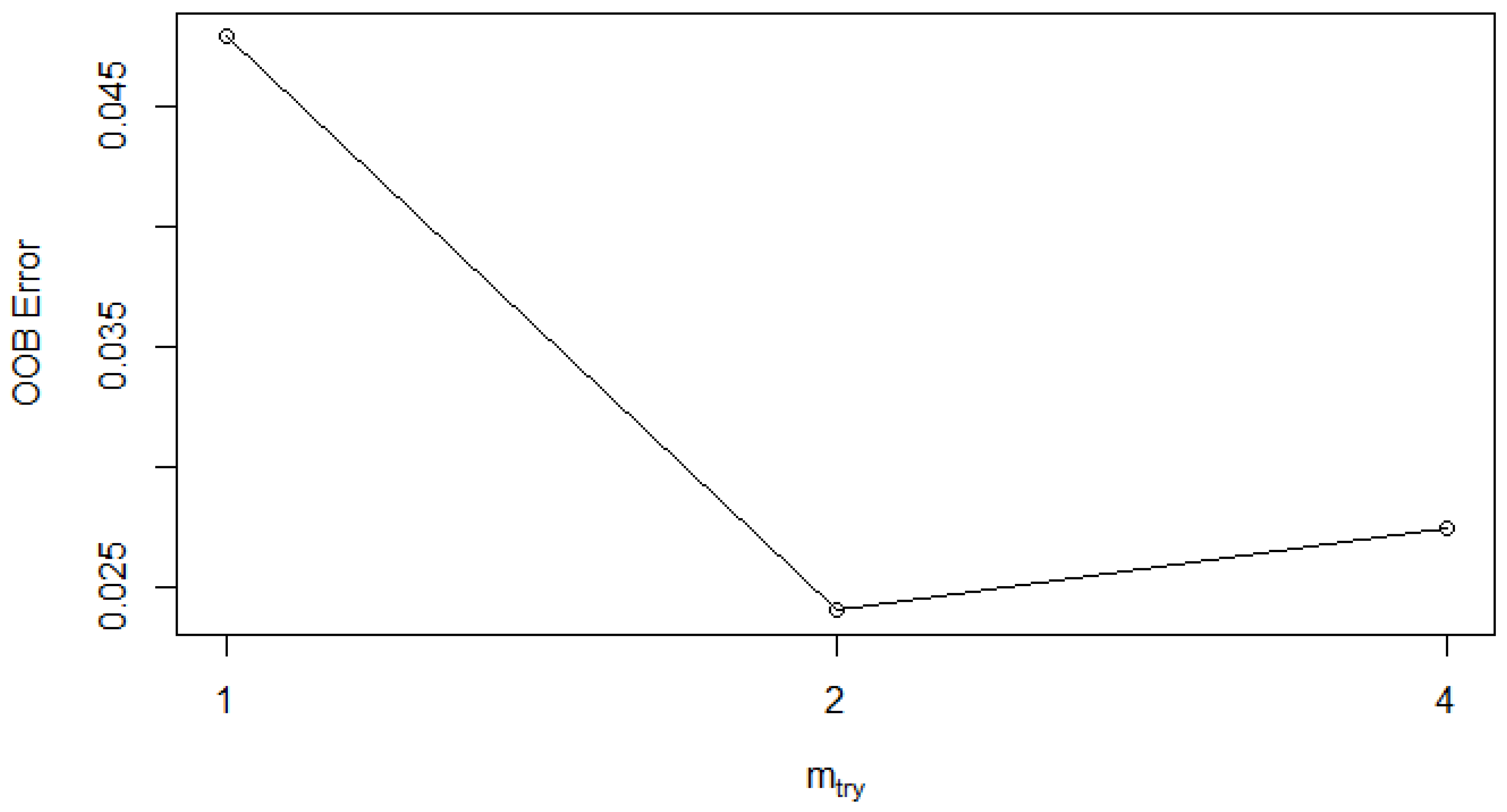
The second parameter that can be optimized in the random forest is the number of features that are randomly chosen for each split. The general rule of thumb is to take the value of the sample size for the number of features as the square root of the total number of features. Tuning can be performed for the number of features (mtry) to be selected per node for splitting. So, it was made sure that the random forest considered the optimal number of features at each node in the tree.
Figure 6 shows the variation in the error rate of the random forest with the sample size of a number of features provided to the decision trees per node. The error rate was initially quite high with mtry at one (4.79%), and then it came down with a mtry value of two and finally increased with a mtry value of four (2.74%). So, the minimum error was 2.4 % at mtry = 2; hence, the sample size used for the number of features per node was two for building the random forest classifier for our dataset, and it was also the default value selected by the random forest [
38].
After building the random forest with the above-optimized values on the training data, it was tested using training and test data. The random forest perfectly classified all the observations of the training data, so the accuracy was 100%. In the case of the test data, one observation was misclassified from both classes. So, for the test data, which consisted of 73 observations, there were only two observations that were misclassified. The correct classification for class ‘HIGH’ was 32 out of 33 observations and for class ‘LOW’ the correct classification was 39 out of a total of 40 observations. The accuracy of the random forest was 97.26%, which was only 3% less than the training accuracy. So, the random forest did not overfit the data, which usually happens in the case of random forest.
A random forest with mtry = p (the number of features) reduces simply to bagging. A random forest with mtry = 7 was also built, which reduced the random forest to a basic bagging technique. Additionally, it was found that the accuracy of the random forest was reduced to 95.89% from 97.26%. So, adding randomness to the features reduced bias in the random forest.
3.6. AdaBoost Boosting
After building the AdaBoost model using the training data, it was given the same training data and test data for its evaluation. The training accuracy for the model was 99.66% with only one misclassified observation. For the AdaBoost model, the accuracy was 94.52% when only two base classifiers were used, 95.89% with three base classifiers, and 97.26% for four base classifiers. So, four base classifiers were considered for final classification with AdaBoost.
3.7. Comparison and Discussion
Table 2 shows the correct and incorrect classifications of the cotton genotypes by various algorithms along with traditional methods of linear discriminant analysis and logistic regression. It can be seen clearly that if the models were evaluated based on accuracy and error rates, then the random forest and the AdaBoost performed the best in classifying the test data with an accuracy of 97.26%; that is, the error was very small, and hence the misclassifications were as well. The next best classifiers were the two algorithms of the decision tree, which behaved identically and had the same accuracy as expected. Because the split criterion used in CART is the Gini impurity and C4.5 makes use of entropy and information gain, both of the measures usually yield similar results. In R software, Gini is the default value where both Gini impurity and entropy are applicable, and this is because entropy might be slower to compute as it makes use of a logarithm.
The next two best performers were the Naïve Bayes and the k-nearest neighbor with only a 1% difference in their accuracy. The worst performer among all the eight classifiers was the linear discriminant analysis, which was expected since it had many assumptions that were definitely violated by the mixed data. Though the accuracy of 83.56% is not that bad, still it is quite less compared to other classifiers, and the rest of everything depends on the application part because some real-life problems can tolerate this much error and other problems such as disease detection require less error in prediction.
The problem that usually occurs in classification or more particularly with machine learning models is overfitting. Overfitting occurs when a model does not perform well with new data. It is characterized by high accuracy for a classifier when evaluated on the training data but low accuracy when evaluated on the test data [
39]. This makes the model useless for the purposes of future classifications. The training and test accuracy are plotted in
Figure 7 and it is clear that there is not much difference between the respective accuracies, and it can be deduced that none of the models were overfitted.
Sensitivity, specificity, and precision for all the methods were calculated using TP, FP, FN, and TN from their respective confusion matrices. The F1 score and G-mean were calculated using specificity, sensitivity, and precision.
Table 3 shows all the calculated performance measures for the eight models.
The accuracy did not reveal much information about how well the classification model actually did in predicting the positive and negative classes independently. If the priority is the positive class and some more misclassification of the negative class can be tolerated, then the model is required to have high sensitivity. That is, in our data, if it is desired to correctly classify high-yielding genotypes only and the model can tolerate the low-yielding genotypes being classified as high, then the classification model with the highest sensitivity will be selected. It can be seen in
Figure 8 that the decision trees, random forest, and AdaBoost have the same sensitivity of 96.97%. These four algorithms were equally good in classifying the high-yielding genotypes with the least misclassifications for class “HIGH”. The rest of the four algorithms had the same order for sensitivity as these had for accuracy, with LDA being the worst.
If the priority class is the class of low-yielding genotypes, then a high value of specificity is desired, which measures how often the negative class is correctly classified. The specificity of random forest and AdaBoost were highest among all models, indicating that these methods were also good at classifying low-yielding genotypes being 97.50% accurate. Both decision trees that had the highest sensitivity and good accuracy performed the worst in classifying the low-yielding genotypes with the least specificity along with LDA. Naïve Bayes, k-NN, and logistic regression had similar performance in terms of specificity.
The next measure was precision, which measures out of all the predicted positives, how many observations were actually positive. It tells us how accurate the model is when it says an observation belongs to the positive class.
Figure 9 represents the recall and precision along with the F1 score and G-mean for the eight classification models. The precision for the models follows the same order as that of specificity; that is, random forest and AdaBoost performed the best with 96.97% precision. Decision trees and LDA performed the worst in terms of precision. The precision of 96.97% tells us that the model was 96.97% accurate with its predictions.
Sensitivity and specificity are used for evaluating the classification models when performance for one class matters. Choosing the best model is sort of balancing between predicting positive and negative classes accurately. So, when it is desired to have good performance for both classes simultaneously, then the F1 score and G-mean are used as performance measures. A good model should have high precision and recall values; the F1 score combines both and gives the harmonic mean of precision and recall, while the G-mean is the geometric mean of sensitivity and specificity. The F1 score and G-mean values were approximately the same for their respective model since both are derived from the same type of measures. The random forest and AdaBoost algorithm were again at the top of the chart in terms of performance, with an F1 score and G-mean value of approximately 97%. The logistic regression and linear discriminant analysis were the bottom two performers.
After checking the performance of the classification models using various performance measures, we can assure that the random forest and AdaBoost models had the highest value for all the performance measures and were lighted as the superior models.
4. Conclusions
Machine learning algorithms proved to be effective in solving problems of classifying cotton genotypes with mixed variables. These algorithms provide a nonparametric alternative to traditionally used methods for the classification of mixed variable data. Machine learning approaches have the advantages that in most machine learning algorithms, data transformation is unnecessary, it can handle missing predictor variables, the success of prediction is not dependent on data meeting normality conditions or covariance homogeneity, variable selection is intrinsic to the methodology, and it provides good accuracy over the traditional methods. The machine learning classifiers that were considered for this study included k-nearest neighbor (k-NN), Naïve Bayes, Classification and Regression Tree (CART), and C4.5 algorithm of the decision tree, random forest, and AdaBoost. The confusion matrices were obtained for all the classifiers according to the number of correct and incorrect classifications. There was not much difference in training and test accuracies, which implied that none of the models were overfitted. The machine learning classifiers were compared with the linear discriminant analysis and the logistic regression, as these two classification models are most widely used in agriculture data and hence were used as the base for comparison.
The random forest and AdaBoost algorithm had the highest value for all the performance measures, which means these models performed in a balanced way with the highest overall accuracy, sensitivity, and specificity at the same time. So, these models were the best at classifying the high- and low-yielding cotton genotypes. The decision trees were the next best classifiers followed by the Naïve Bayes model. It can be concluded that these five models can be used for the classification of cotton genotypes, with priority being random forest because AdaBoost may perform the same as random forest but will take a long time to train if the data are very large. The worst performer among all the eight classifiers was the linear discriminant analysis, which was expected since it has many assumptions which are definitely violated by mixed data.
For data types such as ours, which was sort of balanced and had continuous and categorical variables, the decision tree, random forest, and boosting algorithm performed the best, and instead of traditional methods, these can be used in the future for a similar type of data.


