Abstract
To improve the efficiency of accident treatment on mountain highways and reduce the degree of disruption from traffic accidents, the grading method of the ellipse-like radiation range of traffic accident impact is proposed. First, according to the propagation law of traffic accidents, the general function of mountain highways affected by traffic accidents was constructed based on the Gaussian plume model. Then, based on the gravity field theory, the influence of the accident source point on the accident road was analyzed in the aftermath of a supposed accident. Additionally, considering the cascading failure of the road network, the influence of the accident-intersecting roads was demarcated by the cascading failure load propagation function. Based on this analysis, the ellipse-like radiation range models of traffic accidents on the accident road and the intersecting roads were proposed, respectively. Next, the adjustment parameter was further introduced to incorporate the different levels of influence of traffic accidents on the surrounding road network into the model, and the grading impacts of the accident on the potentially utilized opposite lane were discussed. Finally, according to the queuing theory model, simulation design, and portability analysis, the accuracy of the ellipse-like radiation range grading model was verified. The research results show that, compared with queuing theory and simulation results, the error of the grading model of the ellipse-like radiation range affected by traffic accidents was within a reasonable range; that is, the model can reasonably quantify the difference of traffic accident propagation on the accident road and the intersecting roads. Moreover, the heterogeneity of traffic accident propagation was verified by taking the non-occupied opposite lanes as an example. The grading method of influence radiation range utilized for traffic accidents on mountain highways can quickly provide corresponding auxiliary decision support for accident rescue within varying influence ranges.
1. Introduction
Mountain highways are prone to frequent traffic accidents due to their complex terrain and special geological conditions, a susceptibility which has a substantial negative impact on economic development and people’s health [1,2]. In severe cases, delayed rescue may increase the probability of a secondary accident [3,4]. Therefore, accurately quantifying the radiation range of mountain highway accidents can provide auxiliary decision support for rapid emergency rescue measures, accelerate road congestion evacuation and reduce the impact of accidents.
In the past, most of the research objects relating to traffic accidents have been expressways, which are completely enclosed sections. Once a traffic accident occurs, traffic congestion always spreads only in a fixed direction upstream, rather than forming a diffusion in the area [5]. As opposed to highways, mountain highways always exist in network form. The traffic congestion caused by the accident first spreads upstream in the form of line propagation, and the traffic wave continues to propagate along the intersection to the surrounding road network after reaching the next intersection. That is, the accident’s influence on mountain highways is spread by line-area hierarchical transmission. In addition, most mountain highways do not have central dividers, and the impact may spread to the opposite lanes [6]. Therefore, it is necessary to explore a method suitable for determining the impact range of mountain highway accidents.
Based on the Gaussian plume model, this study proposes a new grading model of the ellipse-like radiation range of traffic accidents suitable for mountain highways, one which divides the impact radiation range of accident-occurrence roads and accident-intersecting roads into three levels. The accuracy of the grading model is verified by comparing it with the queuing theory model and the simulation analysis results, which can effectively simulate the propagation and diffusion law of traffic accidents in mountain road networks. The paper can therefore provide a fundamental theory for reasonably predicting the traffic accident risk level of mountain highways, and then guide the formulation of traffic risk identification and safety prevention and control policies for mountain highways.
The remainder of this paper is organized as follows: Section 2 introduces the previous relevant research on the accident influence range in detail. In Section 3, the calibration of accident influence and the construction of the grading model of accident influence radiation ranges are expounded. In Section 4, the ellipse-like radiation grading range model of accident impact is calculated and compared with the queuing theory model and the simulation results to verify its accuracy and effectiveness. In Section 5, the results of this study are discussed. Finally, the conclusions and further research directions are described in Section 6.
2. Literature Review
2.1. Propagation Mechanism of Accidents Impact
The study of the propagation mechanism of accident impact has been a focus for scholars from various countries, who have been have been unremittingly exploring the dimensions of the question, including: using the accident delay value [7,8] to determine the maximum spatial impact range and congestion duration of the accident [9,10] and capturing the dynamic operation process of accidents and predicting the spatiotemporal evolution caused by accident, which is helpful in measuring the potential impact of accident congestion [11,12]. Further, the degree of congestion caused by an accident can be estimated by detecting the relationship between factors related to the accident or elements of the accident itself (such as the type of accident, the time of the accident, weather conditions, and road conditions) [13,14]. The above studies have enabled traffic managers to take timely and effective traffic organization measures in the case of limited resources to reduce the negative impact of traffic accidents.
The research on the temporal and spatial impact propagation of accidents can further grasp the dynamic evolution process of accidents and help to predict the potential degrees of congestion caused by accidents. Researchers mostly have used the deterministic queuing diagram and the motion wave (shock wave) theory to analyze the influence of accidents on the surrounding road network and the principle of accidents from the perspective of time and space [15,16,17,18]. Moskowitz and Newman first proposed a deterministic queuing graph method to study the impact of the downstream capacity of bottleneck sections, that is, to estimate the cumulative total delay value of vehicles from the queuing graph, but it is difficult to reflect the repeated congestion after the accident [19]; Lawson et al. proposed an improved queuing graph method to measure the spatiotemporal impact of bottlenecks, but there are still limitations in practical applications, especially when capacity changes occur many times [20]. Saeedmanesh and Geroliminis established the deterministic queue length model of expressways based on the arrival rate and departure rate curves and calculated the total delay of accidents, queue length, and congestion duration, but the modeling could not estimate the traffic state in real-time [21]. Barth and Boriboonsomsin carried out the simulation analysis of typical sections of an accident, which provided a way of thinking for the proposal of economic vehicle speed and related research [22]. With the development of big-data technology, most scholars now collect speed data from loop detectors and detection vehicles and estimate the temporal and spatial effects of traffic accidents based on various models, such as the integer programming model [5,17], cellular automata [23], K-nearest neighbor [24], or fuzzy K-means clustering [25].
The research objects of the above literature mostly focus on expressways or accident roads of highways (without considering the spread of accidents to surrounding roads). However, the congestion diffusion caused by accidents in mountain highways often presents a trend of the point, line, and plane spreading, and the operation state of neighbor nodes will also be affected by the accident source point and congestion points. Moreover, the above research methods are mostly based on traffic flow theory or complex network theory, and most studies focus on the construction of a traffic wave propagation model after the traffic accident, and the methods are relatively simple.
In addition, researchers have created a variety of classical research methods and models that can provide theoretical guidance. At the same time, deep learning methods (such as Bayesian networks, convolutional neural networks, spiking neural networks, etc.) have also been gradually introduced into the prediction of the impact range of accident time and space, and the results are also ideal [26,27,28].
2.2. Analysis Method of Accident Influence Range
The method for determining the accident impact range was first extended by the Institute of Traffic Impact Assessment. At present, the most commonly used methods for determining the spatiotemporal impact range of accidents are the road enclosure method [29], the circle extrapolation method [30], and the Gaussian plume model method [31,32]. The above three methods all have their priorities and limitations [33]. The calculation of the road enclosure method is direct, fast, and convenient, but it has weak theoretical support and a strongly subjective particularity. The network structure of the circle extrapolation method is clear and the model form is simple, which can ensure the real-time processing of traffic events to a certain extent. However, there is a certain roughness when selecting the area, and a large number of high-precision data are needed to perform the calculations, which is not particularly suitable for measuring traffic diffusion. The Gaussian plume model is a widely used atmospheric pollutant diffusion model, which is often used to calculate the range of gas diffusion; it is a systematic engineering methodology derived from synergetics with many factors and comprehensiveness [31]. The method is simple and easy for software programming. Meanwhile, the diffusion of traffic congestion caused by accidents in the road network and the diffusion of toxic gases in the atmosphere are similar in theory, which can be applied to determine the scope of traffic accidents through in-depth exploitation.
Integrated with the advantages and disadvantages of the above three types of models, the Gaussian plume model is more suitable for the study of the accident influence radiation range. However, for mountain highways, after the accident, it may make the road section or intersection temporarily interrupted, resulting in cascading failure, which will lead to the different influences of the accident source on the accident road and the intersecting road. Although the Gaussian plume model can simulate the diffusion and propagation of toxic gas in a limited space, its model itself does not fully consider the influence of the traffic operation state of the adjacent nodes and sections of the accident source on the accident source and the difference in the radiation range of its influence on different sections of the road network.
To summarize, it is necessary to form a new idea and method based on previous studies. That is, the cascading failure propagation function is introduced based on the Gaussian plume model, which can more accurately measure the actual influence of the accident source point on the surrounding road network and establish a more realistic analysis model of the radiation range of traffic accidents in the mountain highway. It can not only accurately predict the dynamic influence range of accidents, but also provide the basis for the detection and identification of secondary events [25,34].
3. Methodology
3.1. Foundational Model Construction for Traffic Accident Influence Degree of Mountain Highway
The diffusion of poison gas is affected by external and internal factors such as temperature, light, wind, and limited space boundaries. It is composed of multiple units, and each unit is equivalent to a circle and is assigned to the whole research range. The diagram of its diffusion is shown in Figure 1a. The radiation propagation process of traffic accidents on mountainous highways is similar to the spread of poison gas in space, which is mainly related to the type and intensity of the accident and is proportional to the intensity of traffic accident source points. The influence of roads or intersections within the scope of influence is equal to that of traffic accident units, and the diffusion diagram is shown in Figure 1b.:
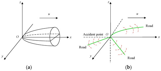
Figure 1.
Traffic accident diffusion diagram evolving from poison gas diffusion: (a) poison gas diffusion diagram, (b) traffic accident diffusion diagram.
In addition, the impact of the accident will also be limited by spatial factors such as whether to set up a central divider and the road occupation of the accident, that is, its influencing factors also include internal and external factors. Given this similarity, based on the Gaussian plume model, this paper determined the influence distance of traffic accidents on the surrounding road network under different influence degrees, that is, the diffusion influence range of traffic accidents on mountainous highways.
The Gaussian plume model of poison gas diffusion was transformed into the basic model of radiation diffusion affected by traffic accidents on mountain highways [35].
where represents the influence of the point accident diffusion source (dimension is 1); is the release rate of the diffusion source; is the average travel speed of traffic flow at the accident source; and are the distribution parameters of traffic volume at the accident point in the y-direction and z-direction, respectively; and represent the horizontal and vertical distances from the accident point (x-direction is defined as the diffusion direction of traffic volume that is the upstream direction of the traffic accident section, y-direction is the vertical direction of x-direction); z is the height of space point.
For the convenience of discussion, the hypothetical model of Equation (2) is simplified: first, the impact of a traffic accident has the same diffusion parameters in the y-direction and z-direction, that is ; second, is a function of x, simplified by Robert as , k is the diffusion coefficient [36]; and third, the road traffic network is a plane, so the size of z is not considered, that is, z = 0, let , and r is the diffusion radius. At this time, Equation (1) is simplified as:
where q, μ, and k are three quantities that need further consideration. Generally, q is related to the type of accident and the condition of the surrounding road network, μ is related to the road traffic condition, and k is related to the accident section. Further assumptions will be made to simplify the problem in the absence of extensive investigations. In Equation (2), since the diffusion coefficient is only related to x, let , a be a constant. Equation (2) can be transformed into:
Let Q be the influence of the accident point on the road, and be the proportion of the diffuse traffic volume at the accident point, with the range of , which is related to the type of accident. It is assumed that after the traffic diffusion at the accident point, at the boundary point in the x-direction, the influence of the accident source point on the sections and intersections is represented by the accident average influence C* before the traffic distribution at the accident section.
In Equation (4), is the influence of diffusion accident, R0 is the equivalent circle radius of the accident area, and S is the accident area. Then:
Substituting Equation (5) into Equation (3), the general function of the degree of impact of traffic accidents on mountain highways is:
For the allocation of traffic volume, only x and y directions are considered, namely , . The value of Q values according to different roads. Therefore, the influence of the road network around the accident needs to be calibrated first.
3.2. Influence Analysis of Mountain Highway Accident Source Point on the Surrounding Road Network
After an accident on a certain road section, the impact on the current accident road section is the largest, until the traffic flow on it is allocated to the intersected road section, and the impact gradually reduces. For intersecting roads, the impact of the accident mainly comes from the additional load transferred from the accident section. The more the load capacity of the intersected road is exceeded, the greater the impact of accidents on the road. Therefore, it is necessary to discuss the influence of the accident point on accident road and intersection road , respectively.
3.2.1. Influence Analysis of Accident-Occurred Road Based on Gravity Field Theory
In this study, the influence of the accident source point on the accident road can be obtained by the gravity field theory simulation, as shown in Equation (7).
where represents the diffusion coefficient; represents the maximum influence distance; means the potential energy of the accident source point, which is a comprehensive index related to the proportion of lanes occupied by the accident, the accident type, the accident vehicle type, and so on.
According to the traffic flow theory, the queue length increases with the increase of wave flow and is affected by the duration of the accident. The accident origin potential energy was converted to the total number of vehicles during the accident duration (the total number of vehicles is the product of traffic wave flow and traffic congestion time ). Based on the traffic wave theory, the calculation formula of is as follows:
and are the velocity and density of the accident upstream traffic flow; and are the velocity and density of the accident downstream traffic flow. Thus, Equation (7) can be converted to Equation (9):
3.2.2. Influence Analysis of Accident-Intersecting Road Considering Cascading Failure
Considering the influence of node failure on the failure degree of road traffic networks, this paper uses the cascading failure load propagation function to explain the influence of the calibration accident point on the intersecting road network.
The construction process of the cascading failure load propagation function of mountain highways is as follows: the driving time of the road section is defined as the weight of the edge, and the directed weighted graph of the road network in the study area is constructed. Where is the set of nodes, is the set of edges, is the weight of edges, .
Step 1: In this study, the initial load is defined by the betweenness of the edge and the actual capacity of the actual road section corresponding to the edge. The initial load of any edge is , and the maximum load capacity of the edge is .
where , , and represent adjustment parameters; denotes the betweenness of the edge ; denotes road capacity of the edge ; is the number of the shortest paths between s and t passing through the edge ; is the number of all shortest paths between s and t.
Step 2: This step considers the propagation of the failed load. When the real-time load of the connected section of any failure section exceeds its load capacity at t time, that is, to meet , the connected section will also fail, and the real-time load is:
where, is the load corresponding to the section at (t − 1) time, .
Step 3: The model then begins redistribution of the failed load. Considering the actual situation, that the driver is unable to quickly obtain all the information in the whole road network, the traffic volume on the failed road section should be preferentially shunted to the road section connected with the accident section according to certain rules. In addition, the section connected with the failure section is divided into two kinds. The first is the adjacent edge which is completely or approximately opposite to the direction of the failure edge; the second is the adjacent edge whose angle with the failure edge direction is less than or close to the right angle, as shown in Figure 2. Assuming that the edge is an invalid edge, the edge is the first kind of adjacent edge of the edge ; edge and edge are the second kinds of adjacent edges of the edge .
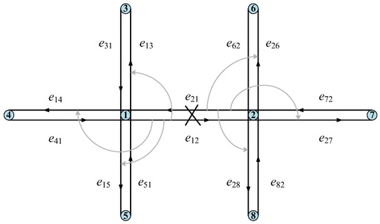
Figure 2.
Cascading failure load distribution diagram.
After the failure of a certain road segment, the driver tends to choose the second type of adjacent edge connected to the failure edge when choosing other paths, while the load diverted to the first type of adjacent edge only accounts for a small proportion. Assuming that the load diverted to the first kind of adjacent edge accounts for times of the total load on the failure edge, the total load allocated to the second kind of adjacent edge accounts for times of the total load on the failure edge, and the corresponding additional load distribution can be calculated respectively as follows: Equations (12) and (13), and each edge of the same type performs load distribution according to its respective weight, as shown in Equation (14).
where is the total load of the failed section; is the first adjacent edge of the failed section; , … are the second adjacent edge of the failed section; is the weight value of the edge ; is the free travel time on the section ; is the traffic flow in the section ; is the capacity of the section ; and are the parameters of the BPR function.
The specific example is as follows: assuming that is the total load to be allocated on the failed edge , and and are the extra loads allocated to edge and edge respectively, the extra loads can be calculated as , and .
Step 4: The model then assigns a grading of the failed load. There are generally two types of section failure in mountain highways: destructive failure and congestion failure. The former refers to a certain road section that is destroyed completely and cannot be repaired in a short time, so all the loads on the adjacent road section are distributed after the failure of the road section. The latter is that a certain road section is blocked, but it still can pass vehicles. And the failure section will not transfer all the loads to adjacent sections, but instead, only transfer some loads exceeding their maximum capacity. Then, the load p allocated at the failure edge at time t: destructive failure is , congestion failure is .
Step 5: The process creates the cascading failure impact assessment index . Combined with the actual situation of each road section under mountain highway accidents, the failure condition of the accident section was determined. Aiming at the failure degree of the accident section in intersecting roads (the second type of adjacent edge), the corresponding cascading failure impact assessment index model H was constructed as follows:
where, is the real-time load of the road section , is the load capacity of the road section , is the moment when the load is allocated to the adjacent section, and is the regulation parameter.
The cascading failure impact assessment index H of the road section when the load is assigned to the adjacent road section is used as the influence of the accident diffusion source on the road section, namely .
3.3. Ellipse-Like Radiation Range Model Construction of Accidents Impact of Mountain Highway
3.3.1. Accident-Occurred Road Model
To improve accuracy, the diffusion radius r of the model should not be too large, and the value range is (i = 1,2,…,6) [31,32], and r obeys the normal distribution. At the confidence level of 0.95, the confidence interval is , and when , . To further simplify the model, this study evaluates the influence of the distance from the accident source point x by using the influence degree (the average value of ) of the traffic volume at the accident point on the section allocated to the surrounding road network.
Set as the ultimate influence of the accident source on the surrounding road network, and let :
Substitute Equation (8) into Equation (17) to obtain the maximum impact distance of the accident source point on the accident road:
Combined with traffic flow theory, the model was modified as follows:
- (1)
- According to Equation (19), the maximum influence distance is when the influence degree of the accident source point on the accident road is different levels (u = 1, 2, …N).
- (2)
- represents the degree of influence of traffic accidents on the maximum influence range of mountain highways, which is related to the proportion of lanes occupied by the accident, the type of accidents, and the type of accident vehicles, and it can be determined by trial calculation of actual accident data. The adjustment parameter can take the values of 1, 0.3, 0.05 [31], and .
- (3)
- The proportion of the diffusion traffic volume at the accident point is , and its value range is (0, 1), which is determined by the nature of the accident. The calibration of the proportional constant is related to the proportion of lanes occupied by accidents and the type of accidents, .
In summary, the maximum range under different influence degrees of the accident point on the accident road is:
where let , , , the corresponding , , can be obtained, and the corresponding , , are the maximum influence distance when the influence degree of the accident source point on the accident road is first, second and third.
3.3.2. Accident-Intersecting Road Model
Based on the analysis in Section 3.2.2, the influence of the accident diffusion source on the intersecting road j can be obtained, and Equation (14) can be transformed into Equation (21):
Substituting Equation (21) into Equation (6), the propagation model of influence range of accident-intersecting road based on cascading failure can be obtained as follows:
When the influence degree of the accident source point on the intersecting road is determined to be different levels of , the corresponding maximum influence distance is:
where is the intersecting road number; is the horizontal distance from the intersecting road to the accident source point; is the maximum influence distance of the accident source point on the diffusion under different influence levels of the intersecting road ; is the influence of the accident diffusion source on the intersecting road .
C takes , and , corresponding to , , and , respectively, which are the maximum influence distances when the diffusion influence degree of the accident source point on the intersecting road is first, second and third.
3.3.3. Grading Discussion of Ellipse-Like Radiation Range
The influence of traffic accidents on mountain highways is quite different in the distribution of accident roads and intersecting roads. Because the accident influence mainly spreads along the current road, the influence range of the current road direction is much larger than that of the intersecting road. Considering the shape of the influence range, with the accident location as the origin, the influence range of the accident is in an ellipse-like shape.
Moreover, there are two cases of mountain highway accidents. One is that the accident only takes up the directional lane, and the vehicle operation of the directional lane is affected, while the opposite lane is still running normally. At this time, the accident influence only spreads upstream of the accident point. The other is that the accident takes up both the directional lane and the opposite lane. At this time, the traffic flow in the opposite lane will also be congested, and the accident influence will spread upstream and downstream of the accident point.
According to Formulas (20) and (2), the maximum influence distances corresponding to the first-level, second-level, and third-level accident influence degrees are calculated, and the corresponding distance points with the same influence degree are smoothly connected in turn. Thus, the accident influence area is divided into first-level, second-level, and third-level influence areas, each of which directly represents the size and scope of the accident influence. The schematic diagram of the ellipse-like impact range of the accident given both unaffected and affected opposite lanes is shown in Figure 3.
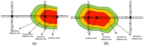
Figure 3.
Accident influence ranges schematic: (a) unaffected opposite lanes, (b) affected opposite lanes.
4. Case Study
4.1. Traffic Accident Data
A traffic accident in the Nan’an section of National Road G324 in Quanzhou, Fujian Province was analyzed. The National Road G324 is the main road to undertake the vehicle diversion task of the Shenhai-Zhangzhou Expressway extension project, of which the Nan’an Section is about 25.90 km long. The accident was located between the starting point K212 + 840 and the endpoint K223 + 840 sections. The whole line adopts the secondary highway standard of four two-way lanes, and the proportion of lanes occupied by the accident was 0.5. No relevant traffic warning signs were set after the accident. The accident data related to the accident point is shown in Table 1.

Table 1.
Accident point-relevant data.
Flow Calculation at Each Stage after the Accident. According to the Van Aerde model [19] and traffic wave theory [20], the flow and wave velocity of continuous traffic flow can be calculated, respectively, based on the data in Table 1. The calculated traffic flow at each stage after the accident is shown in Table 2.
Table 2.
Traffic flow at each stage after the accident.
Accident Duration and Queue Length Calculation. After the occurrence of accidents, due to the processing and removal of accidents often needing a certain time, the process of accident impact continuation will generally experience the following stages: accident discovery and response, accident removal, and traffic recovery. Based on the propagation characteristics of traffic waves [20], the propagation process of traffic waves upstream after the accident can be obtained. It can be judged that the accident detection and response time was , and the accident clearing time was . Then, the maximum duration of accident was , and the maximum queue length was 258 m.
4.2. Ellipse-like Radiation Range Calculation of Accident Impact of Mountain Highway
The accident section number is ①, and the upstream section number is ②. There is an intersecting road (road section ③ and road section ④) 136 m away from the accident location. The road network diagram of the accident example is shown in Figure 4.
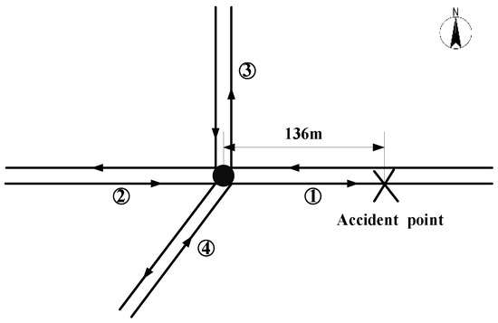
Figure 4.
Intersecting road-relation diagram of accident’s upstream node.
4.2.1. Accident Occurred Road Range Calculation
Taking the above traffic accident as an example, according to Equation (19) , the corresponding maximum impact distance can be determined when the impact degree of the accident source point on the accident road is at different levels of .
Where, ; the total number of vehicles with accident duration in the incident section is ; through the trial calculation of actual accident data , so as to obtain (), (), (); combined with the actual situation in the selected road network, the parameter value in Equation (19) is , .
To sum up, it can be determined that the maximum influence distances corresponding to different levels of are , , and , which indicates that the maximum influence distances are 271 m, 479 m, and 715 m respectively, when the influence degree of the accident source on the accident road is first, second and third levels.
4.2.2. Accident-Intersecting Road Range Calculation
The cascading failure process and failure influence results of the accident-intersecting roads were as follows:
Step 1 is the definition and calculation of the initial load. Based on Equation (9), taking , , , the betweenness , and the calibration capacity [37], the initial load and the maximum load capacity can be determined.
Step 2 determines the weight of the edges. Taking , , the weight , are determined by Equation (13).
Step 3 performs the distribution and calculation of the failure load. At time , the load of the failure section is assigned to the connected road according to Equation (12), and the load of the road at time is calculated by combining Equation (10), where ε is , and , .
Step 4 transfers the calculation of the accident diffusion source to the intersecting roads. Based on steps 1–3, the cascading failure impact assessment index of each road is calculated. In this case, the congestion failure occurred in the accident section, and the load distribution was to allocate the failure load to the second adjacent side. According to Equations (14)–(15), the influence of the accident diffusion source on the road section can be obtained, and the for the intersecting ③, and the for the intersecting ④.
According to the propagation of the accident on intersecting roads, taking , , , and substituting into Equation (22): ()(), the maximum influence distance can be determined when the influence of the accident source point on the intersecting road is at different levels of , as follows:
, , and , which indicates the maximum influence distances of the accident source in the first, second and third levels of the intersecting road ③ are 269 m, 456 m, and 521 m, respectively.
, , and , which indicates the maximum influence distances of the accident source in the first, second and third levels of the intersecting road ④ are 340 m, 485 m, and 561 m, respectively.
4.2.3. Ellipse-Like Radiation Grading Range Confirmation
The accident considered in this study only occupies the directional lane and does not influence the normal operation of the opposite lanes. The corresponding distance points with the same influence degree are smoothly connected in turn, so the accident-affected radiation range is divided into first-level, second-level, and third-level influence areas. The ellipse-like radiation range diagram of accident influence is shown in Figure 5.
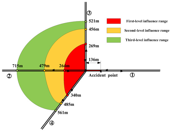
Figure 5.
Accident influence range diagram.
4.3. Model Validation
4.3.1. Simulation Experiment
Taking a traffic accident in the Nan’an section of national road G324 in Quanzhou, Fujian province as an example, the relevant parameters in the Vissim software (version 7.0) traffic simulation were determined according to the accident scene:
- (1)
- Fundamental parameters: The two intersecting roads are both composed of four two-way lanes, with a vehicle running speed of 50 km/h, a minimum headway spacing of 2 m, an average parking distance of 1.5 m, a maximum deceleration of forced lane change of −4 m/s2, and the waiting time for lane change is 60 s. A total of 390 detectors were set up to detect the real-time speed and other data of roads near the accident point, including 120 at the south entrance, 150 at the west entrance, and 120 at the north entrance, with a detector interval of 10 m. According to the actual situation of road operation, the turning ratios of each entrance road at the intersection were as follows: the north and south entrance road were 0.2 (straight), 0.4 (left), 0.4 (right), and the west entrance road was 0.8 (straight), 0.1 (left), 0.1 (right).
- (2)
- Accident parameters: The accident occurred on the east exit road 136 m away from the intersection at 300 s, with an accident-occupied lanes proportion of 0.5 (the accident occupied the outermost lane), an accident duration of 1 h, and an accident length of 20 m. Therefore, the length of the closed lane (the length of the accident area) was set to 20 m; the deceleration zone was set to 0–50 m west of the accident location, and the lane speed near the accident area was 15 km/h; the two-lane speed at 50 m to 70 m west of the accident location was set to 20 km/h; the same-direction lane of the accident (length 20 m) and west 20 m, east 20 m (a total of 60 m) were all deceleration zones, where the speed was set to 6 km/h. After the accident treatment was completed, the deceleration zone was removed to achieve the purpose of evacuating the accident-queuing traffic. The specific schematic diagram is shown in Figure 6.
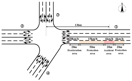 Figure 6. Simulation parameter-setting diagram of accident section.
Determination method of influence range grading: The simulation results are mainly: speed, acceleration, deceleration, and the number of passing vehicles at each detection point (60 s output once). The corresponding first-level, second-level, and third-level influence ranges are mainly determined by speed. The first-level influence range corresponds to the maximum queuing length of the accident propagation, that is, the longest distance detector position with the corresponding speed of 0 to 10 km/h within a certain period, and there is basically no vehicle passing through the detection point. The second-level influence range corresponds to the farthest detector position where the speed is stable at 85% operating speed (10 to 42.5 km/h), and a small number of vehicles pass through this detection point. The third-level influence range corresponds to the farthest detection point where the speed basically reaches the normal operation speed (50 km/h and above), and the vehicles at the detection point pass normally.
4.3.2. Model and Simulation Results Comparison
In this study, three methods are used to calculate the corresponding impact range after the accident, and the specific results are shown in Table 3.
Table 3.
Models and simulation results of accident influence ranges (unit: m).
The first-level influence range analysis of the accident road section ② was undertaken comparatively under the three methods. The queuing theory model (Model 1) was used to calculate the maximum queuing length of the accident section (road section ②) as 258 m (where the queuing length is the actual queuing length minus 136 m from the intersection), which is the corresponding first-level influence range; the first-level influence range is 264 m and 280 m (the latter occurs within the 2660 s time period) calculated by accident influence radiation range (Model 2) and the Simulation Method, respectively.
Based on the influence range of queuing theory model (Model 1), the rationality of the first-level influence range of Model 2 and the Simulation Method is verified by relative error analysis. The relative error σ calculation Equation (24) is as follows [38]:
where refers to the influence range of the model to be verified, and refers to the influence range of the benchmark model.
It can be seen that the errors of the first-level influence range of Model 2 and simulation results are 2.33% and 4.65%, respectively, compared with Model 1 (Table 4). The relative error of the two is within the allowable range (the relative error within ± 5% indicates that the calculation result is reasonable) [38], and Model 1 is more accurate than the simulation result (2.33% less than 4.65%, the smaller the relative error, the more accurate the result).
Table 4.
Relative error of each model of first-level influence range in road section ②.
The comparative analysis of Model 2 and simulation results: Based on the Simulation Method, the rationality of the influence range of three levels of Model 2 is further verified. Through the relative error calculation Equation (24), it can be obtained from the data in Table 3 that the relative errors of the three levels influence ranges of Model 2 and the simulation results are within 5% (see Table 5), which further verifies the effectiveness of the model proposed in this study [38]. Taking road section ③ as an example, the influence ranges of the three levels obtained by Model 2 are 269 m, 456 m, and 521 m, respectively; and the influence ranges of the three levels are 290 m (3080 s), 450 m (3440 s), and 510 m (3600 s) by using the Simulation Method. Thus, the errors of all levels’ influence ranges calculated by Model 2 and the Simulation Method are: 3.92%, 1.33%, and 2.15%, respectively; that is, the errors are within a reasonable range. Similarly, the relative errors of the second-level and third-level influence range of road section ② and the three influence ranges of road section ④ are within a reasonable range.
Table 5.
Relative error of three levels’ influence ranges model for each road section.
4.4. Model Portability
The above case analysis is only for the same sample data, and the road network node upstream of the accident is a cross intersection. In order to improve the universality of the model, it is necessary to analyze the portability of the model, that is, so that the classification model of traffic accident impact range proposed in this study can be applied to other mountain highways. Therefore, this paper takes a traffic accident in the Heyang section of national highway G108 in Weinan City, Shaanxi Province as an example (the road network node upstream of the accident is the Y-type intersection) to further verify the applicability of this model.
The accident occurred on a road that adopts the secondary highway standard, two-way four lanes, and the proportion of lanes occupied by the accident is 0.5. The road network diagram of the accident example (G108) is shown in Figure 7. And the accident section number is ⑤, and the upstream section number is ⑥. There is an intersecting road (road section ⑦) 78 m away from the accident location.
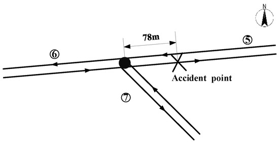
Figure 7.
Intersecting road relation diagram of accident upstream node (G108).
Model 1, Model 2, and the Simulation Method calculate the accident impact radiation range as follows:
Model 1 (queuing theory model): Based on the propagation characteristics of traffic waves [20], the propagation process of traffic waves upstream after the accident can be obtained. It can be judged that the accident detection and response time is , and the accident clearing time is . The maximum duration of accident is then , and the maximum queue length is 211 m.
Model 2 (radiation range model of accident influence): According to the calculation process in Section 3.3, the first-level, second-level and third-level influence ranges of the accident road (section ⑥) are 209 m, 393 m, and 595 m respectively; The first-level, second-level and third-level influence ranges of the accident-intersecting road (section ⑦) are 218 m, 384 m and 474 m, respectively. The ellipse-like radiation range diagram of accident influence is shown in Figure 8.
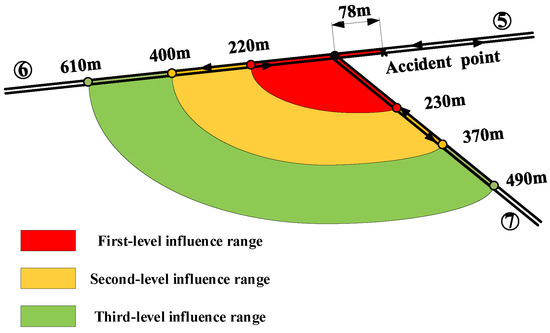
Figure 8.
Accident influence range diagram (G108).
The Simulation Method: A total of 270 detectors were set up to detect the real-time speed and other data of roads near the accident point, including 120 at the south entrance, 150 at the west entrance, with a detector interval of 10 m. According to the actual situation of road operation, the turning ratios of each entrance road at the intersection as follows: the south entrance road was 0.5 (left), 0.5 (right), and the west entrance road was 0.8 (straight), 0.2 (left). The specific schematic diagram is shown in Figure 9.
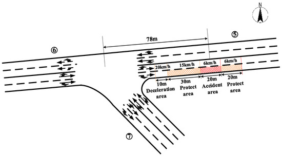
Figure 9.
Simulation parameter-setting diagram of accident section (G108).
The accident influence range and relative error analysis results of the above three methods are shown in Table 6, Table 7 and Table 8, respectively.
Table 6.
Models and simulation results of accident influence ranges (unit: m).
Table 7.
Relative error of each model of first-level influence range in section② (G108).
Table 8.
Relative error of three levels influence ranges model for each section (G108).
Similar to the analysis method in Section 4.3.2, the errors of the first-level influence range of Model 2 and simulation results are 0.95% and 4.26%, respectively, compared with Model 1 (Table 7). The relative error of the two is within the allowable range (the relative error within 100% ± 5% indicates that the calculation result is reasonable) [38]. Additionally, Model 1 is more accurate than the simulation result (0.95% less than 4.26%, the smaller the relative error, the more accurate the result).
The comparative analysis of Model 2 and simulation results: Based on the Simulation Method, the rationality of the influence range of three levels of Model 2 is further verified. Through the relative error calculation Equation (24), it can be obtained from the data in Table 6 that the relative errors of the three levels influence ranges of Model 2 and the simulation results are within 5% (Table 8), which further verifies the effectiveness of the model proposed in this study [38].
Therefore, it can be seen that the model proposed in this study is not only suitable for accident-propagation analysis when the accident upstream road network node is the cross intersection but is also applicable to the special intersection (Y-type intersection), that is to say, to a certain extent, the model has certain portability.
5. Discussion
This study proposes a new traffic accident influence radiation range grading model that can effectively simulate the propagation and diffusion law of accidents in mountain highway networks, and uses queuing theory (Model 1) and the Simulation Method to verify the accuracy and portability of the proposed model (Model 2).
From the comparative analysis results of the two cases in the paper, it can be seen that, since the queuing theory only can calculate the maximum queuing length of the current road of the accident (that is, the first-level accident influence range), Model 1 is first selected as the benchmark model to determine the rationality of Model 2 and the Simulation Method. The relative-error comparison results show that the error between Model 2 and Model 1 is much smaller than that of the Simulation Method. Specifically, the reason for the error of the former may be that according to the actual situation of the accident, its influence range will be affected by the flow, duration, and so on [17,18]. At the same time, different accidents have different degrees of influence on the road network, which will lead to different calibrations of the ultimate influence of the accident source point on the road network in Model 2. Therefore, the above factors will cause some errors in the application of Model 2. This result is similar to the error caused by the maximum distance calculation results in [31], which determine that the development project has different effects on the surrounding road network. The deviation caused by the latter may be mainly due to the setting of parameters such as driving behavior, acceleration and deceleration, and detector spacing (fixed 10 m) in the simulation. In particular, the detector spacing is fixed at 10 m, so that the influence range of the simulation results at all levels is a multiple of 10 (that is, 1–9 values are missing between every 10 digits). Therefore, to a certain extent, the error of the latter is larger than that of the former, and the setting spacing of the detection points can be further reduced to simulate the influence range of the accident more accurately. Similar to the VISSIM simulation experiment error in References [15,38], which also found that the set distance of the detector will cause a certain error in the model, and the error does not affect the accuracy of the results. Moreover, since Model 1 cannot calculate the second-level and third-level influence range, simulation results can only be selected as the benchmark model to verify the rationality of Model 2. Similarly, the relative errors of the influence range of the three levels of each section calculated by Model 2 are within 5%, that is, the error is also within a reasonable range. The error interpretation of Model 2 and simulation results is the same as above. In general, the errors are within the allowable range, indicating that the accident-affected radiation range model and the Simulation Method proposed in this study are both effective.
Compared with the existing methods for determining the range of accident influence, the contributions of this study lie in the following aspects: Firstly, the ellipse-like traffic accident impact grading model proposed in this study divides the traffic accident impact area into three levels. Through the range length of the three levels, the congestion degree of each level range can be reflected laterally, and the evolution process of accident influence can be clarified more carefully. Secondly, this paper has developed an improved Gaussian smoke model to determine the influence range of the accident, which is not limited to calculating the influence range of the accident road, but also integrates the cascading failure effect of the intersecting road into the influence range calculation model, so as to more accurately determine the impact degree of the accident on the upstream adjacent road network [39]. Thirdly, beyond attention to the maximum queue length after the accident (first-level influence range), that is, beyond the basis of queuing theory calculation, the ultimate influence of the accident source point on the road network is included in the model. The difference in the adjustment coefficient reflects the difference in the propagation of traffic accidents in different influence levels on the road, and accurately reflects the heterogeneity of the spatial propagation of accidents [21]. Finally, the different levels of accidents are closely related to traffic flow and speed, that is, according to the grade of road congestion at different levels, traffic managers can take targeted and effective measures respectively for the three accident influence levels to accelerate the congestion evacuation and reduce the negative impact of traffic accidents [17,39]. For example, for a section with a large first-level impact range, accident warning signs can be set up in advance at an upstream intersection near the third-level impact range, and vehicles can be guided to other roads nearby to minimize the input of traffic flow in the accident section [2]. For the first-level and second-level influence ranges, before entering the two influence ranges respectively, according to the actual situation, the running speed of the vehicle is limited by the on-site traffic guidance, so as to avoid queue jumping and other phenomena aggravating the congestion of the accident sections. Meanwhile, the speed can be gradually controlled in the downstream section of the bottleneck to accelerate the congestion evacuation [5].
6. Conclusions
Based on the Gaussian plume model, this study proposed a grading model of ellipse-like radiation range applicable to the traffic accident influence on mountain highways. Different from the existing single accident impact range determination, the proposed model can divide the influence range of traffic accidents into three influence levels, which can reflect the congestion severity of different influence levels after the accident. It can be seen that the classification range of accident impact determined by the model can reasonably reflect the propagation of accident impact on mountain highways.
In this study, the concept of the Gaussian plume model is abstracted and modified, and the foundational model of the influence degree of traffic accidents on mountain highways is constructed. Moreover, the different effects of accident source points on the occurrence road and accident-intersecting road are carefully considered. On this basis, according to the difference in influence radiation range of traffic accidents caused by accident location, road operation state, and other factors, the influence degree of each accident section is divided into three levels by introducing adjustment parameters. The queuing theory and simulation method are used to verify the model in this paper, and the model portability is further analyzed by using the accident data of another mountain highway to verify that the grading model has a certain accuracy and effectiveness. Therefore, the model of this study can sufficiently demonstrate the propagation and diffusion law of the impact of traffic accidents and can take corresponding emergency rescue measures for different impact levels (for example, managers can formulate corresponding warnings, guidance, evacuation, and other measures before the vehicle enters different influence levels) to keep the impact of the accident within a controllable range, accelerate road congestion and evacuation, and avoid the occurrence of secondary accidents. It can be seen that this study has broad application prospects in the fields of traffic guidance, congestion control, and prevention caused by accidents, and can provide a basis for phased traffic safety management of mountain highways.
In addition, the ellipse-like radiation range grading model of traffic accident influence proposed in this paper has certain limitations. On the one hand, the model only considers two cases of accident impact involving and not involving opposite lanes (one-way road blocking and two-way road-blocking). When the actual traffic accident occurs, the accident occupancy situation is different, and the corresponding bottleneck point will also be affected by the type of accident, the time of the accident, the weather condition, and the road condition [5]. In particular, many studies have confirmed that bad weather is an important factor affecting the traffic safety of mountain highways [13,14]. Therefore, in future research, on the basis of ensuring that the accident is sufficient according to the data, the above factors of the accident point should be further statistically analyzed, which can help to determine the key factors affecting the impact of traffic events on the induced congestion, and to analyze the scope of the accident in more detail to further improve the accuracy of the model. Based on this, traffic managers can take more effective measures to reduce the negative impact of traffic accidents.
Author Contributions
Conceptualization, J.W. and S.W.; methodology, J.W., S.W. and D.L.; validation, J.W., S.W. and C.M.; writing—original draft preparation, J.W. and S.W.; writing—review and editing, J.W., S.W. and X.L.; visualization, D.L. and P.L.; supervision, X.L. All authors have read and agreed to the published version of the manuscript.
Funding
This research was funded by the Natural Science Basic Research Program of Shaanxi Province, China (Grant no. 2021JQ-276) and the Projects Supported by Special Funds for Urban Construction (Grant no. SZJJ2019-22).
Institutional Review Board Statement
Not applicable.
Informed Consent Statement
Not applicable.
Data Availability Statement
Some or all data, or models that support the findings of this study are available from the corresponding author upon reasonable request.
Conflicts of Interest
The authors declare no conflict of interest.
References
- Yu, B.; Chen, Y.R.; Bao, S.; Xu, D. Quantifying Drivers’ Visual Perception to Analyze Accident-prone Locations on Two-lane Mountain Highways. Accid. Anal. Prev. 2018, 119, 122–130. [Google Scholar] [CrossRef]
- Wang, J.J.; Cao, X.D. System Analysis of Potential Accidents on Mountain Road Based on Rough Set and Quantitative Theory. KSCE J. Civ. Eng. 2021, 25, 1031–1042. [Google Scholar] [CrossRef]
- Xu, J.; Lin, W.; Wang, X.; Shao, Y.M. Acceleration and Deceleration Calibration of Operating Speed Prediction Models for Two-lane Mountain Highways. J. Transp. Eng. Part A Syst. 2017, 143, 04017024. [Google Scholar] [CrossRef]
- Zhang, H.; Zhang, M.; Zhang, C.; Hou, L. Formulating a GIS-based Geometric Design Quality Assessment Model for Mountain Highways. Accid. Anal. Prev. 2021, 157, 106172. [Google Scholar] [CrossRef] [PubMed]
- Wang, Z.L.; Qi, X.; Jiang, H. Estimating the Spatiotemporal Impact of Traffic Incidents: An Integer Programming Approach Consistent with the Propogation of Shockwaves. Transp. Res. Part B Methodol. 2018, 111, 356–369. [Google Scholar] [CrossRef]
- Yuan, Z.; Huang, D.; Tong, W.; Liu, Z. Characteristic Analysis and Prediction of Traffic Accidents in the Multiethnic Plateau Mountain Area. J. Transp. Eng. Part A Syst. 2020, 146, 04020068. [Google Scholar] [CrossRef]
- Lu, C.; Elefteriadou, L. An Investigation of Freeway Capacity Before and During Incidents. Transp. Lett. Int. J. Transp. Res. 2013, 5, 144–153. [Google Scholar] [CrossRef]
- Almotahari, A.; Yazici, M.A.; Mudigonda, S.; Kamga, C. Analysis of Incident-induced Capacity Reductions for Improved Delay Estimation. J. Transp. Eng. Part A Syst. 2019, 145, 04018083. [Google Scholar] [CrossRef]
- Hojati, A.T.; Ferreira, L.; Washington, S.; Charles, P. Hazard Based Models for Freeway Traffic Incident Duration. Accid. Anal. Prev. 2013, 52, 171–181. [Google Scholar] [CrossRef] [PubMed]
- Hojati, A.T.; Ferreira, L.; Washington, S.; Charles, P.; Shobeirinejad, A. Modelling Total Duration of Traffic Incidents Including Incident Detection and Recovery Time. Accid. Anal. Prev. 2014, 71, 296–305. [Google Scholar] [CrossRef]
- Lan, C.L.; Venkatanarayana, R.; Fontaine, M.D. Development of a Methodology for Determining Statewide Recurring and Nonrecurring Freeway Congestion: Virginia Case Study. Transp. Res. Rec. 2019, 2673, 566–578. [Google Scholar] [CrossRef]
- Wang, J.H.; Xie, W.J.; Liu, B.Y.; Fang, S.; Raglandbc, D.R. Identification of Freeway Secondary Accidents with Traffic Shock Wave Detected by Loop Detectors. Saf. Sci. 2016, 87, 195–201. [Google Scholar] [CrossRef]
- Shannon, D.; Murphy, F.; Mullins, M.; Eggert, J. Applying Crash Data to Injury Claims-an Investigation of Determinant Factors in Severe Motor Vehicle Accidents. Accid. Anal. Prev. 2018, 113, 244–256. [Google Scholar] [CrossRef] [PubMed]
- Tainter, F.; Fitzpatrick, C.; Gazillo, J.; Riessman, R.; Knodler, M., Jr. Using a Novel Data Linkage Approach to Investigate Potential Reductions in Motor Vehicle Crash Severity—An Evaluation of Strategic Highway Safety Plan Emphasis Areas. J. Safety Res. 2020, 74, 9–15. [Google Scholar] [CrossRef]
- Liu, L.; Zhu, L.; Yang, D. Modeling and Simulation of the Car-truck Heterogeneous Traffic Flow Based on a Nonlinear Car-Following Model. App. Math. Comput. 2016, 273, 706–717. [Google Scholar] [CrossRef]
- Khatak, A.; Wang, X.; Zhang, H. Incident Management Integration Tool: Dynamically Predicting Incident Durations, Secondary Incident Occurrence and Incident Delays. IET Intell. Transp. Sy. 2012, 6, 204–214. [Google Scholar] [CrossRef]
- Chung, Y.; Recker, W.W. Frailty Models for the Estimation of Spatiotemporally Maximum Congested Impact Information on Freeway Accidents. IEEE Trans. Intell. Transp. Syst. 2015, 16, 2104–2112. [Google Scholar] [CrossRef]
- Chung, Y. Identification of Critical Factors for Non-recurrent Congestion Induced by Urban Freeway Crashes and Its Mitigating Strategies. Sustainability 2017, 9, 2331. [Google Scholar] [CrossRef]
- Moskowitz, K.; Newman, L. Notes on Freeway Capacity, 3rd ed.; California Division of Highways: Sacramento, CA, USA, 1962.
- Lawson, T.W.; Lovell, D.J.; Daganzo, C.F. Using Input-output Diagram to Determine Spatial and Temporal Extents of a Queue Upstream of a Bottleneck. Transp. Res. Rec. 1997, 1572, 140–147. [Google Scholar] [CrossRef]
- Saeedmanesh, M.; Geroliminis, N. Dynamic Clustering and Propagation of Congestion in Heterogeneously Congested Urban Traffic Network. Transp. Res. Part B Methodol. 2017, 105, 193–211. [Google Scholar] [CrossRef]
- Barth, M.; Boriboonsomsin, K. Energy and Emissions Impacts of a Freeway-based Dynamic Eco-driving System. Transp. Res. Part D Transp. Environ. 2009, 14, 400–410. [Google Scholar] [CrossRef]
- Kong, D.; Sen, L.; Li, J.; Xu, Y. Modeling Cars and Trucks in the Heterogeneous Traffic Based on Car-truck Combination Effect Using Cellular Automata. Phys. A 2021, 562, 125–329. [Google Scholar] [CrossRef]
- Chen, Q.J.; Song, X.; Yamada, H.; Shibasaki, R. Learning Deep Representation from Big and Heterogeneous Data for Traffic Accident Inference. In Proceedings of the 2016 30th AAAI Conference on Artificial Intelligence (AAAI-16), Phoenix, AZ, USA, 12–17 February 2016; pp. 338–344. [Google Scholar]
- Yang, H.; Wang, Z.; Xie, K.; Dai, D. Use of Ubiquitous Probe Vehicle Data for Identifying Secondary Crashes. Transp. Res. Part C Emerg. Technol. 2017, 82, 138–160. [Google Scholar] [CrossRef]
- Chen, Z.; Liu, X.C.; Zhang, G. Non-recurrent Congestion Analysis Using Data-driven Spatiotemporal Approach for Information Construction. Transp. Res. Part C Emerg. Technol. 2016, 71, 19–31. [Google Scholar] [CrossRef]
- Najjar, A.; Kaneko, S.; Miyanaga, Y. Combining Satellite Imagery and Open Data to Map Road Safety. In Proceedings of the 2017 31th AAAI Conference on Artificial Intelligence (AAAI-17), San Francisco, CA, USA, 4–9 February 2017; pp. 4524–4530. [Google Scholar]
- Li, P.; Abdel-Aty, M.; Yuan, J. Real-time Crash Risk Prediction on Arterials Based on LSTM-CNN. Accid. Anal. Prev. 2020, 135, 105371. [Google Scholar] [CrossRef]
- MOHURD (Ministry of Housing and Urban-Rural Development of the People’s Republic of China). Technical Guidelibnes for Traffic Impact Analysis of Construction Project(R); MOHURD: Beijing, China, 2010.
- Fan, X. Application of Spherical Extrapolation Method to TIA. Comput. Comm. 2007, 25, 137–140. [Google Scholar]
- Wang, L.; Liu, X.M.; Ren, F.T. Cloud Model of Deciding Study Area in Traffic Impact Analysis. China J. Highw. Transp. 2001, 14, 100–105. [Google Scholar]
- Abdel-Wahab, M.; Essa, K.M.; Embaby, M.; Elsaid, S.M. Some Characteristic Parameters of Gaussian Plume Model. Mausam 2012, 63, 123–128. [Google Scholar] [CrossRef]
- Ma, G.; Zheng, C.; Wan, X. Determination of the Scope of Traffic Incident. Adv. Mech. Eng. 2017, 9. [Google Scholar] [CrossRef]
- Yang, H.; Wang, Z.; Xie, K.; Ozbay, K.; Imprialou, M. Methodological Evolution and Frontiers of Identifying, Modeling and Preventing Secondary Crashes on Highways. Accid. Anal. Prev. 2018, 117, 40–54. [Google Scholar] [CrossRef]
- Fallah-Shorshani, M.; Shekarrizfard, M.; Hatzopoulou, M. Evaluation of Regional and Local Atmospheric Dispersion Models for the Analysis of Traffic-related Air Pollution in Urban Areas. Atmos. Environ. 2017, 167, 270–282. [Google Scholar] [CrossRef]
- SBQTS (State Bureau of Quality and Technical Supervision); SBEPA (State Environmental Protection Administration). Technical Methods for Making Local Emission Standards of Air Pollutants. SBQTS: Beijing, China; SBEPA: Beijing, China, 1991. [Google Scholar]
- MTPRC (Ministry of Transport of the People’s Republic of China). Technical Standard of Highway Engineering; MOHURD: Beijing, China, 2014.
- Huang, F.; Liu, P.; Yu, H.; Wang, W. Identifying if VISSIM simulation model and SSAM provide reasonable estimates for field measured traffic conflicts at signalized intersections. Accid. Anal. Prev. 2013, 50, 1014–1024. [Google Scholar] [CrossRef] [PubMed]
- Zheng, Z.; Qi, X.; Wang, Z.; Ran, B. Incorporating Multiple Congestion Levels Into Spatiotemporal Analysis for the Impact of a Traffic Incident. Accid. Anal. Prev. 2021, 159, 106255. [Google Scholar] [CrossRef] [PubMed]


Publisher’s Note: MDPI stays neutral with regard to jurisdictional claims in published maps and institutional affiliations. |
© 2022 by the authors. Licensee MDPI, Basel, Switzerland. This article is an open access article distributed under the terms and conditions of the Creative Commons Attribution (CC BY) license (https://creativecommons.org/licenses/by/4.0/).