Local Sustainability Performance and Its Spatial Interdependency in Urbanizing Java Island: The Case of Jakarta-Bandung Mega Urban Region

Abstract

Jakarta–Bandung Mega Urban Region (JBMUR), located in the western part of Java Island, Indonesia, is experiencing rapid regional development which can be observed from its increase in population density, massive changes of land-use from agricultural land into built-up area, rapid development of infrastructure and facilities, and advances in economic activities. Unfortunately, problems related to sustainability emerge along with this rapid regional development, primarily in decrease in environmental quality and social performance, leading to unsustainable development. This study aims: (1) to develop indicators promoting sustainable development at the subdistrict level, named the local sustainability index (LSI), utilizing factor analysis; (2) to observe local-scale spatial interdependency by employing local indicator of spatial association (LISA) statistics; and (3) to identify regional clusters based on LSI scores using K-means clustering method. Our LISA results show that spatial interdependency of local sustainability performances exists between local-scale spatial units: the LSI of a subdistrict is influenced by the sustainability state of the surrounding areas. Meanwhile, the clustering results show that most subdistricts in JBMUR are categorized as members of cluster 1 with low LSI values in economic and social dimensions but moderate in environmental dimensions.

1. Introduction

Sustainability has been a general perspective in regional development [1]. This perspective recognizes that human’s social and economic needs are constrained by environment and technology [2]. The term “sustainable development” is popular in current development discourses driven by limited natural resources and increased environmental damage [3,4]. There have been a lot of definitions of sustainable development. The well-known definition is that provided by the Brundtland Commission in 1987 [1,5,6,7,8]: a development that seeks to meet the needs of the present generation without reducing the ability to meet future needs [9,10,11]. Afterwards, various concepts have followed to comply with this terminology, including value change, moral development, social reorganization, and transformational process towards a better world in the future.

There are three pillars in the construction of sustainable development: economy, society, and ecology [12,13,14,15,16]. More precisely, the sustainable paradigm guides public policy to be formulated based on the selection of development alternatives that are not only economically feasible, but also ecologically friendly, and socially acceptable [17]. This paradigm emphasizes equity principles between the three pillars [9,18].

Although the theoretical concept of sustainability is widely accepted, measures to quantify a sustainable state are yet to be developed continuously [19,20]. Policymakers require timely information to build measures that demonstrates whether the current system is heading to a sustainable state or not [21]. Such measure can be represented by indicators quantitatively able [22,23,24,25] to assess policies [17], infrastructures [26], socioeconomic factors [27], resource uses [28], emissions [29], and other attributes contributing to and profit from the region’s metabolism, prosperity, and quality of life [30,31,32].

An indicator is a variable that may describe one characteristic of the state of a system. It is commonly presented through observed or estimated data [33]. Sustainable development indicators are needed to guide policies and decisions at all levels, whether at the village, city, district, state, region, nation, continent, or worldwide level [34,35]. Previously, The Compendium of Sustainable Development Indicator Initiatives, hosted and managed by the International Institute for Sustainable Development, lists over 500 sustainability indicators, of which 67 indicators are for global scope, 103 are for national scope, 72 are for state or provincial scope, and 289 are for local or metropolitan scope [36].

The ability to estimate the relationship between environmental conditions and human wellbeing [37,38] is a fundamental factor of a good indicator. An indicator does not necessarily include all sustainability aspects since they often become subjective and meaningless [21]. In addition to indicators, indices are also needed to quantify sustainability and supervise several aspects of development subsequently. In general, “indices” are statistical indicators that provide appropriate quantitative information that simplifies analysis of the phenomenon under study. An “index” is a quantitative aggregation of many indicators. It can provide a view of a multidimensional, simplified, and coherent system [39]. Indices normally give a static overview of a system [40]. When calculated occasionally, indices can indicate the tendency of the system whether it becomes more sustainable or not and highlight the driving factors that are most responsible. Sets of indicators and their aggregation into indices are increasingly used to drive policy decisions [35,39].

Indicators and indices for sustainable development have been widely discussed at the regional, national, and global levels [41,42] but still discussed very limitedly at the local level [43,44,45,46,47]. Some argue that studies at the regional, national, and global levels tend to be economically biased. Meanwhile limited studies at the local level do not only focus on economic, but also on environmental and social indicators [48]. Specifically, spatial dependency between locations is stronger at the local level rather than national or global level. The sustainability performance of a location is influenced by sustainability conditions of its surrounding [49]. The enactment of the Law on Village Autonomy in Indonesia requires a formulation of sustainable development indicators at the village level [50,51]. These indicators are expected to be used as measuring tools and guidance for local authority policymakers in implementing development programs.

In Java Island of Indonesia, the establishment of the sustainability index and indicators has become crucial. Java Island covers merely 6.7 percent of Indonesia’s land [52] and is where built-up areas are concentrated, housing approximately 43% of Indonesia’s population [53]. The island is experiencing rapid urban development, followed by many social and environmental problems, such as poverty and natural disasters [54]. Among the regions in Java Island, Jakarta-Bandung Mega Urban Region (JBMUR) has experienced the most rapid growth, urbanization, social problems, and environmental destruction [55]. JBMUR is formed as a result of urban area expansion of two metropolitan areas, namely Jakarta metropolitan area and Bandung metropolitan area. Jabodetabek’s expansion is more dominant [56]. Its contribution to the national gross domestic product (GDP) reaches more than 25% [57]. The region’s development has focused less on sustainability aspects, where several parts of the region have low sustainability index [49,58].

The aims of this research are: (1) to develop indicators promoting sustainable development in JBMUR at the subdistrict level, named the local sustainability index (LSI) utilizing factor analysis; (2) to observe local-scale spatial interdependency of LSI by employing local indicator of spatial association (LISA) statistics; and (3) to identify regional clusters based on the LSI value of the three sustainability dimensions using the K-means clustering method.

2. Materials and Methods

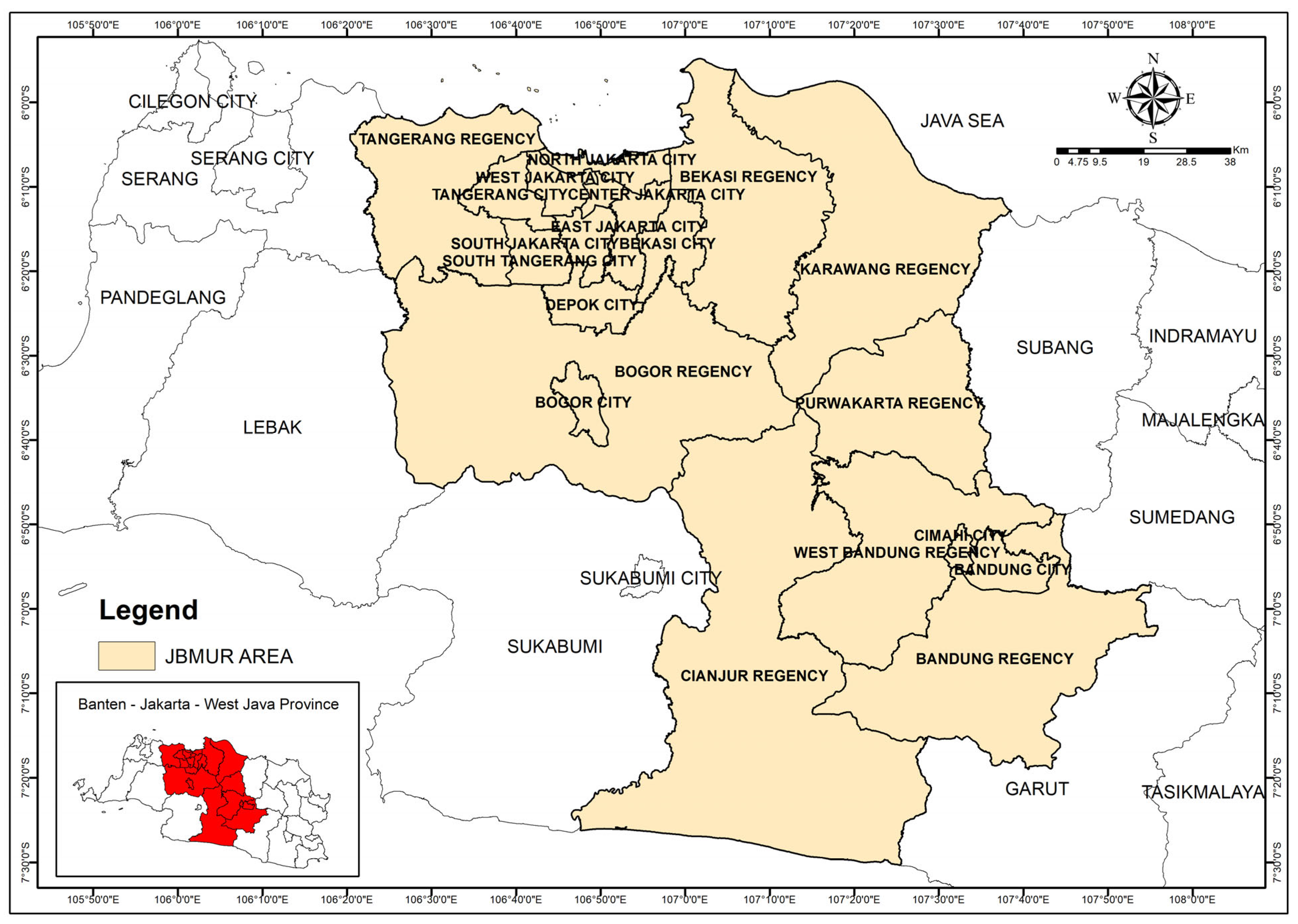
2.1. Study Area

This study focuses on building sustainability indicators and indexes at JBMUR [50,59]. Geographically, this region is located between 5°55′ to 7°30′ South latitude and 106°20′ to 107°55′ East longitude, with a total area of 16,607.29 km². JBMUR is formed as a result of urban area expansion of the Jakarta metropolitan area (also known as Jabodetabek) and the Bandung metropolitan area (also known as Bandung Raya). Jakarta is the capital of Indonesia and Bandung is the capital of West Java province. In total, JBMUR covers 8 regencies and 12 municipalities. The regencies are Bogor, Purwakarta, Cianjur, Bandung Barat, Bandung, Karawang, Bekasi, and Tangerang. Meanwhile, the municipalities are West Jakarta, North Jakarta, East Jakarta, South Jakarta, Center Jakarta, South Tangerang, Tangerang, Bogor, Bekasi, Depok, Cimahi, and Bandung (Figure 1). JBMUR consists of 335 kecamatan (subdistricts) and 2954 desa (villages). Our analysis is at subdistrict level.

2.2. Methods

One of the challenges faced in developing local sustainability variables in this research is the availability of data at the local level. In this research, we strongly depend on Data Potensi Desa or Data Podes, literally translated as Village Potential data, collected by Statistics Indonesia. Village Potential data are collected routinely 3 times in a period of 10 years to support the Population Census, Agricultural Census, or Economic Census activities. Statistics Indonesia has carried out Village Potential data census 2018 in all regencies/municipalities, subdistricts, and village level government administration areas. The results of this census are data concerning availability of infrastructure, social and economic potential owned by villages, subdistricts, regencies/municipalities throughout Indonesia. Thus, important facts related to the availability of infrastructure and the potential possessed by each region can be monitored on a regular basis and continuously [50,59]. The Village Potential data used in this research are the latest data available, collected in 2018.

LSI is a development sustainability index at the local level which was first developed by the author in 2016 within the study area in the Greater Jakarta Metropolitan Area (Jabodetabek) with a unit of analysis per village (desa). After being tested in the Jabodetabek metropolitan area, this index has also begun to be tested in several other areas that have various characteristics with different units of analysis using several modified variables or indicators.

From Village Potential data, the local sustainability index (LSI) was developed based on 50 variables (indicators) which were grouped according to the three sustainability dimensions: economy (17 variables), social (19 variables), and environment (14 variables). We filtered and selected relevant variables to describe sustainability. Village Potential data provides data at village level, but then, in this research, data are aggregated and adjusted to subdistrict level.

LSI was developed by employing factor analysis (FA) to select the variables/indicators [49,60]. FA is a statistical method that aims to describe the variability between observed variables and correlated variables. The potential unobserved (underlying) variables are referred to as factors, which are lesser in number than the observed variables. FA looks for combined variation in response to unobserved latent variables [49,60]. Factor loading of a variable measures the extent to which a variable is related to a particular factor [49,60]. The general rationale behind FA is that the information obtained about the interdependencies between the observed variables can be used later to reduce the set of variables in the data set.

FA is used to develop a composite index of each dimension based on factor scores and factor loadings [60,61]. The number of factors is determined by eigenvalues > 1. This method is suitable in our case due to the variability of data measurement unit. The 50 variables included in factor analysis (FA) model are listed in

Table 1. List of variables included in Factor Analysis (FA) model.

Code	Variables
	Economic dimension (k = 1)
V1	Average distance to railway station (km)
V2	Length to the nearest bank (km)
V3	Length to the nearest market (km)
V4	Length to the central business district (CBD) (km)
V5	Length to the nearest city (km)
V6	Number of restaurants and food stalls (per 1000 population)
V7	Number of hotels and lodgings (per 1000 population)
V8	Percentage of built-up area (%)
V9	Infrastructure index
V10	Average distance to toll road (km)
V11	Number of industries other than retails (per 1000 population)
V12	Households using electricity (%)
V13	Average distance to shopping center (km)
V14	Average distance to the village head office center (km)
V15	Number of minimarkets, shops, and markets (per 1000 population)
V16	Cooperatives and banks (per 1000 population)
V17	Regional revenue (PAD) (million rupiahs)
	Social dimension (k = 2)
V18	Mean length to formal education facilities (from kindergarten to university) (km)
V19	Health facilities (hospitals, doctors, pharmacies, clinics, health centers) (per 1000 population)
V20	Mean length to health facilities (hospitals, pharmacies, clinics, health centers) (km)
V21	Medical personnel (per 1000 population)
V22	Diarrhea and vomiting sufferer (per 1000 population)
V23	Dengue fever sufferer (per 1000 population)
V24	Respiratory tract infection sufferer (per 1000 population)
V25	Toddler deaths (per 1000 population)
V26	Maternal mortalities (per 1000 population)
V27	Indonesian labor forces (TKI) (%)
V28	Poor people (%)
V29	Formal education facilities (from kindergarten to university) (per 1000 population)
V30	Measles sufferer (per 1000 population)
V31	Malaria sufferer (per 1000 population)
V32	Tuberculosis sufferer (per 1000 population)
V33	Malnutrition sufferer (per 1000 population)
V34	Mortalities (per 1000 population)
V35	Criminalities (evidence)
V36	Population density (people/km2)
	Environmental dimension (k = 3)
V37	Forest (%)
V38	Plantation (%)
V39	Swamp, ponds, and water body (%)
V40	Percentage of rice field (%)
V41	Percentage of other agricultural area (%)
V42	Rice-field land conversion into non-agricultural land (ha)
V43	Non-rice-field land conversion into non-agricultural land (ha)
V44	Percentage of households living in riparian river (%)
V45	Landslide events (evidence)
V46	Floods events (evidence)
V47	Flash floods events (evidence)
V48	Earthquakes events (evidence)
V49	Whirlwind events (evidence)
V50	Forest fire events (evidence)

.

The FA model is as follows:

$$LS{I}_{ki}={\displaystyle {{\displaystyle \sum }}_{m=1}^{n_k}}{E}_{km}.S_{kmi}$$

(1)

where:

• LSI_𝑘𝑖 is LSI for kth dimension on ith subdistrict;
• k is dimension (1 for economy; 2 for social; 3 for environment);
• E_km is eigenvalue for kth dimension on mth factor;
• S_kmi is factor score for kth dimension, mth factor on ith subdistrict;
• and i is 1, 2, 3, …, n.

To standardize LSI value on a scale of 0–100, we used the following formulation to produce standardized LSI value on a 0–100 scale (LSI_ki (std)):

$$LS{I}_{ki}\left(std\right)=\left(LS{I}_{ki}-LS{I}_{ki}\left(min\right)\right)\left(\frac{100}{LS{I}_{ki}\left(max\right)-LS{I}_{ki}\left(min\right)}\right)$$

(2)

Then, after LSI is obtained, a weight or contiguity matrix based on shapefiles’ polygon proximity is employed to impose a neighborhood structure of the data. It is to assess the degree of similarity among locations and values. The methods used were Global and Local Moran’s I (LISA statistics) with the formula as follows:

$$I=\frac{{{\displaystyle \sum }}_{i=1}^n{W}_{ij}\left(LS{I}_{ki}-\overline{LS{I}_k}\right)\left(LS{I}_{kj}-\overline{LS{I}_k}\right)}{Z_{LS{I}_k}^2{{\displaystyle \sum }}_{i=1}^n{{\displaystyle \sum }}_{j=1}^n{W}_{ij}}$$

(3)

$$I_i=\frac{{{\displaystyle \sum }}_{i=1}^n{W}_{ij}\left(LS{I}_{ki}-\overline{LS{I}_k}\right)\left(LS{I}_{kj}-\overline{LS{I}_k}\right)}{Z_{LS{I}_k}^2{{\displaystyle \sum }}_{j=1}^n{W}_{ij}}$$

(4)

where:

• I is Global Moran’s Index; I_i is Local Moran’s I;
• LSI_𝑘𝑖 is the value of LSI for kth dimension on ith subdistrict;
• LSI_k is the mean of LSI_k;
• W_ij is contiguity matrix reflecting the proximity of subdistrict i’s and subdistrict j’s locations;
• n is the number of subdistricts;
• and $Z_{LS{I}_k}^2$ is the LSI_k‘s variance.

After calculating the value of the local sustainability index (LSI) of economy (LSIeco), social (LSIsoc), and environment (LSIenv), cluster analysis was employed in this study to identify the typologies of subdistricts in JBMUR based on local sustainability performance. Clustering is one of the most common exploratory data analysis techniques used to get an intuition about the structure of the data. It can be defined as the task of identifying subgroups in the data such that data points in the same subgroup (cluster) are very similar while data points in different clusters are very different (minimizing variance within group/cluster and maximizing variance between groups/clusters). Cluster analysis is a tool or technique to group similar observation into a number of clusters based on the observed values of several variables for each individual. In cluster analysis, a large number of methods are available for classifying objects on the basis of their (dis)similarities. Several well-performed methods in cluster analysis include Ward’s minimum variance method and average linkage cluster analysis (two hierarchical methods), and k-means relocation analysis based on a reasonable start classification [62]. Cluster analysis can be a powerful statistical tool to classify or to create regional typologies based on their similar characteristics as shown in some research [63,64,65,66,67,68,69,70,71,72,73].

In this research, we employed multivariate analysis using the K-means clustering method, a non-hierarchical method. This technique is commonly used when clustering a large data rather than clustering using a hierarchical one. The K means clustering algorithm divides a set of n observations into k clusters. K means clustering forms the groups in a manner that minimizes the variances between the data points and the cluster’s centroid. In this study, the distance measure used in clustering analysis is Euclidean distance. Data used were values resulted from LSI in each three dimensions (LSIeco, LSIsoc, and LSIenv). Cluster analysis in this study was run in Statistica 8.0 (Statsoft, Tulsa, OK, USA). The clusters members were displayed spatially using ArcGIS 10.3 (ESRI, Redlands, CA, USA). The number of clusters is determined by silhouette method [74].

3. Results and Discussion

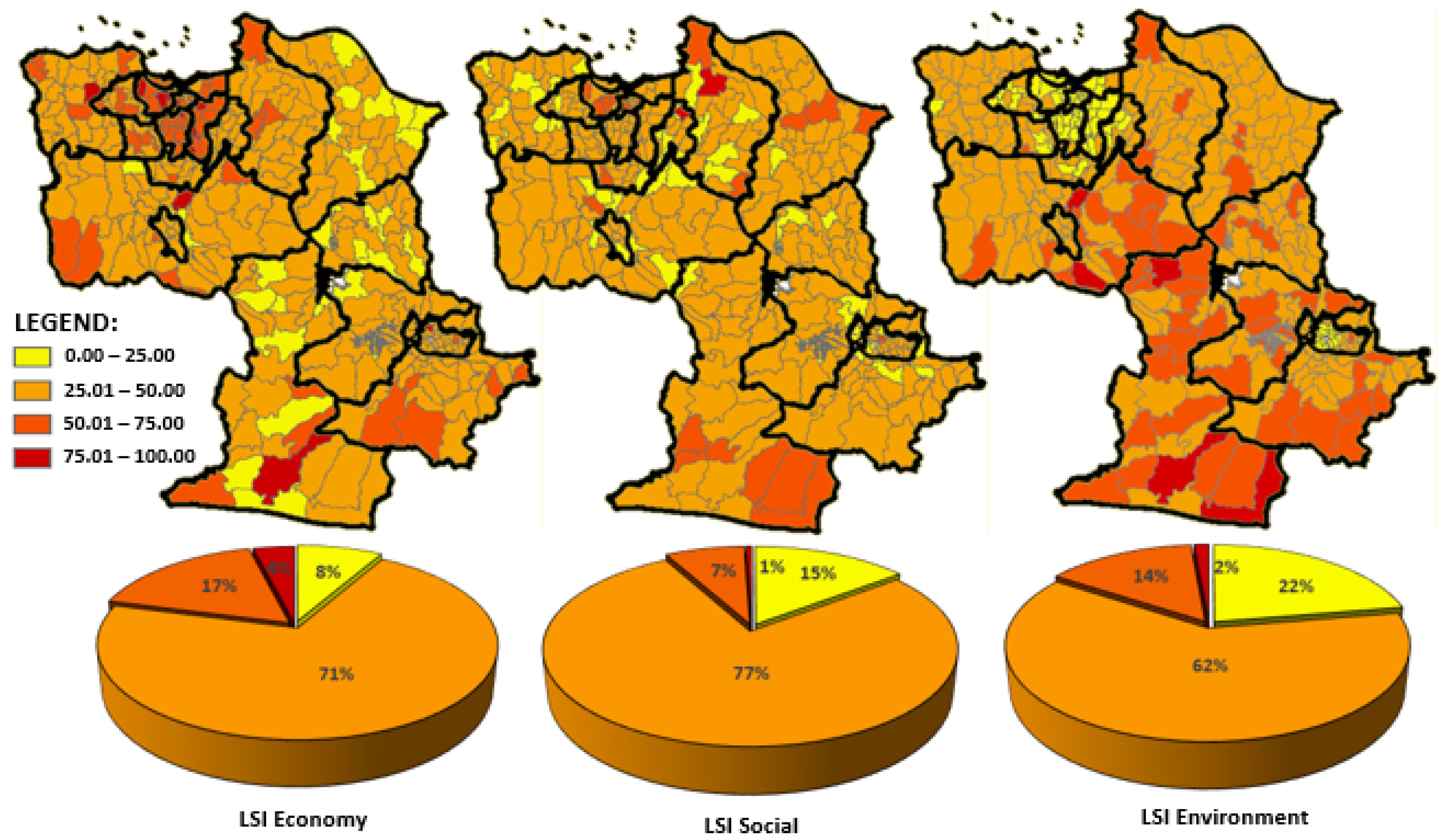
3.1. Local Sustainability Index

To assess the sustainability performance of the region, appropriate indicators are often developed for the use of analysis and decision makers [75]. In this research, we develop the local sustainability index to identify sustainability performance at the subdistrict level of JBMUR. Factor analysis (FA) was used to select key performance indicators/variables of economy (LSIeco), social (LSIsoc), and environment (LSIenv) to form the local sustainability index (LSI). Factor analysis is a technique or statistical method that is used to describe variability among observed, correlated variables in terms of a potentially lower number of unobserved variables called factors. FA can reduce a large number of variables into fewer numbers of factors. In this research, FA which was conducted to determine a composite index for each dimension resulted in a different number of factors. Each factor captures a certain amount of the overall variance in the observed variables, and the factors are always listed in order of how much variation they explain [76,77,78].

Every factor has their own eigenvalue. The eigenvalue is a measure of how much of the common variance of the observed variables a factor explains. Any factor with an eigenvalue ≥ 1 explains more variance than a single observed variable. Eigenvalues measure the amount of variation in the total sample accounted for by each factor. The ratio of eigenvalues is the ratio of explanatory importance of the factors with respect to the variables. If a factor has a low eigenvalue, then it is contributing little to the explanation of variances in the variables and may be ignored as less important than the factors with higher eigenvalues [76,79]. The factors that explain the least amount of variance are generally discarded. Variables representing each factor of the three dimensions are shown on

Table 2. Factor loading of economic factor analysis.

Var	Factor 1	Factor 2	Factor 3	Factor 4	Factor 5
V1	−0.003	−0.073	−0.026	0.876	−0.103
V2	0.803	−0.125	0.103	−0.055	−0.021
V3	0.623	0.046	−0.092	0.017	−0.118
V4	0.814	−0.148	−0.027	0.228	0.132
V5	0.765	−0.197	0.134	0.197	0.208
V6	−0.082	0.126	0.758	0.250	0.062
V7	0.185	−0.075	0.336	−0.281	−0.321
V8	−0.109	0.880	−0.134	0.028	−0.189
V9	−0.119	0.650	0.069	−0.145	0.530
V10	0.141	−0.170	0.103	0.830	0.051
V11	0.233	−0.108	0.016	−0.015	0.880
V12	−0.027	0.893	0.078	−0.113	0.009
V13	0.769	−0.052	0.060	−0.009	0.223
V14	0.837	0.059	0.020	0.100	−0.084
V15	0.346	0.026	0.749	0.063	0.038
V16	−0.184	−0.165	0.668	−0.273	−0.063
V17	0.215	0.044	−0.021	0.268	0.033
Expl.Var	3.916	2.177	1.776	1.887	1.349
Prp.Totl	0.230	0.128	0.104	0.111	0.079
Eigenvalue	4.339	2.119	1.769	1.619	1.259
% total	25.524	12.465	10.405	9.522	7.406
Cumulative	25.524	37.989	48.394	57.916	65.322

,

Table 3. Factor loading of social factor analysis.

Var	Factor 1	Factor 2	Factor 3	Factor 4	Factor 5	Factor 6
V18	0.197	−0.044	0.277	0.023	0.619	0.081
V19	0.807	0.001	0.069	−0.030	0.019	−0.122
V20	0.268	0.076	−0.094	−0.009	0.136	0.727
V21	0.731	0.026	0.101	−0.008	0.025	0.282
V22	0.030	0.935	−0.002	0.070	−0.037	−0.014
V23	0.097	0.541	−0.121	0.459	−0.228	0.185
V24	−0.033	0.910	−0.040	−0.041	0.060	−0.095
V25	0.526	0.030	0.075	0.082	0.272	−0.187
V26	0.324	−0.059	−0.071	0.008	0.352	−0.239
V27	0.149	−0.050	−0.079	0.100	0.733	0.001
V28	0.022	0.048	−0.808	0.018	−0.095	0.109
V29	0.881	0.054	0.007	0.035	−0.005	0.051
V30	0.052	0.080	0.010	0.868	0.013	−0.035
V31	0.000	−0.036	0.040	0.802	0.175	0.057
V32	0.187	0.260	0.049	0.370	−0.275	−0.358
V33	0.195	0.086	0.075	−0.063	0.129	−0.622
V34	0.616	−0.035	−0.132	0.179	0.346	−0.034
V35	0.098	−0.118	−0.346	0.072	−0.364	−0.022
V36	−0.162	0.078	−0.818	−0.089	0.040	0.065
Expl.Var	2.979	2.120	1.602	1.819	1.581	1.305
Prp.Totl	0.157	0.112	0.084	0.096	0.083	0.069
Eigenvalue	3.381	2.429	1.710	1.527	1.231	1.128
% total	17.795	12.787	8.999	8.035	6.477	5.939
Cumulative	17.795	30.582	39.581	47.616	54.093	60.033

and

Table 4. Factor loading of environmental factor analysis.

Var	Factor 1	Factor 2	Factor 3	Factor 4	Factor 5
V37	0.698	−0.032	0.048	−0.035	0.066
V38	0.866	0.041	−0.034	0.093	−0.032
V39	−0.180	−0.043	0.041	0.741	−0.042
V40	0.440	−0.069	0.145	0.715	0.062
V41	0.566	0.202	−0.097	0.353	0.148
V42	0.018	0.877	0.073	0.009	0.015
V43	0.104	0.874	0.039	−0.087	−0.017
V44	0.159	0.046	0.026	−0.040	−0.875
V45	0.674	0.109	0.399	−0.135	−0.034
V46	−0.046	−0.023	0.724	0.301	−0.157
V47	0.227	−0.091	0.762	−0.099	0.058
V48	0.592	0.020	0.488	−0.129	0.078
V49	−0.011	0.305	0.652	0.073	0.025
V50	0.243	0.038	0.001	−0.028	0.476
Expl.Var	2.738	1.701	1.970	1.346	1.061
Prp.Totl	0.196	0.122	0.141	0.096	0.076
Eigenvalue	3.281	1.678	1.570	1.263	1.024
% Total	23.436	11.984	11.212	9.023	7.317
Cumulative	23.436	35.420	46.632	55.654	62.971

, respectively, marked in red.

Based on FA results for economic dimension, FA determined five factors from seventeen variables representing LSIeco. Variables representing each factor are shown on Table 2, marked in red. According to the factor loading’s values, factor 1 is represented by distance to the nearest bank (V2), distance to CBD (V4), length to the nearest city (V5), the average distance to the shopping center (V13), and average distance to the village head office center (V14). These indicators were related to accessibility to economic facilities. Factor 2 is represented by built-up area (V8) and households using electricity (V12). Factor 3 is proxied by the number of food stalls and restaurants (V6) and the number of markets, minimarkets, and shops per 1000 population (V15). Factor 4 is composed of the average distance to railways station (V1) and the average distance to toll road (V10). Factor 5 is represented by the number of industries (V11). The eigenvalue of factor 1 is higher than the eigenvalue of factor 2. The eigenvalue of factor 2 is higher than the eigenvalue of factor 3, etc. In this case, the eigenvalue of factor 1 is the highest (4.339), while the eigenvalue of factor 5 is the lowest (1.259). It means that factor 1 has highest contribution to the explanation of variances in the variables representing the local sustainability index for economic dimension (LSIeco). Table 2 below show the factor loading of economic factor analysis. Factor loading itself is basically the correlation coefficient for the variable and factor. Factor loading shows the variance explained by the variable on that particular factor. Regarding the social dimension, FA established six factors representing LSIsoc, as shown in Table 3. Factor 1 is represented by health facilities (V19), medical personnel (V21), and the number of formal education facilities (V29). Factor 2 is represented by people suffering from diarrhea and vomiting (V22), and people suffering from respiratory tract infection (V24), which reflected the local communities’ health. Factor 3 is represented by poverty (V28) and population density (V36). Factor 4 is represented by people suffering from measles per 1000 population (V30) and people suffering from malaria (V31). Factor 5 is represented by Indonesian labor forces (TKI) (V27), while factor 6 is represented by the mean distance to health facilities (V20). Based on Table 3, it can be seen that the eigenvalue of factor 1 is the highest (3.381), while the eigenvalue of factor 6 is the lowest (1.128). This means that factor 1 has highest contribution to the explanation of variances in the variables representing the local sustainability index for social dimension (LSIsoc). Table 3 below show the factor loading of social factor analysis.

Related to the environmental dimension/aspects, based on the factor analysis results, five factors from ten variables represent LSIenv, as shown in Table 4. Factor 1 is represented by plantation area (V38). Factor 2 is composed of rice-field-to-non-agricultural land conversion (V42) and non-rice-field-to-non-agricultural land conversion (V43). Factor 3 is represented by the floods events (V46) and flash floods events (V47). Factor 4 is represented by the swamps, ponds and water bodies (V39), and rice fields (V40). Factor 5 is represented by households living in the riparian river (V44). Based on Table 4, it can be seen that the eigenvalue of factor 1 (3.281) > factor 2 (1.678) > factor 3 (1.570) > factor 4 (1.263) > factor 5 (1.024). In this FA result for LSIenv, factor 1 has highest contribution to the explanation of variances in the variables representing the local sustainability index for environmental dimension (LSIenv). Table 4 below show the factor loading of environmental factor analysis.

Figure 2 shows the spatial distribution values of LSIeco, LSIsoc, and LSIenv in the Jakarta-Bandung Mega Urban Region (JBMUR). As shown in Figure 2, higher values of the LSIeco are concentrated in the municipalities of Jakarta Province. Some high values appeared as well in several subdistricts in Bandung City and its surrounding region. This pattern indicates that these regions enjoyed better economic performance compared to others. The diagram in Figure 2 displays that only 4% of the total subdistricts in JBMUR have high LSIeco value (between 75.01–100.00), and 71% of subdistricts have moderate values (between 25.01–50.00). As for LSIsoc, 77% of subdistricts have low values (between 25.01–50.00), and only 1% have high values (75.01–100.00). The opposite condition applies for LSIenv, where most subdistricts have high values (14% of subdistricts have index scores between 50.01–75.00 and 62% subdistricts have index between 25.01–50.00). Most subdistricts in Jakarta Province have low values of LSIenv, while on the other hand, many subdistricts in Bogor, Cianjur, and Bandung Regency have high values of LSIenv.

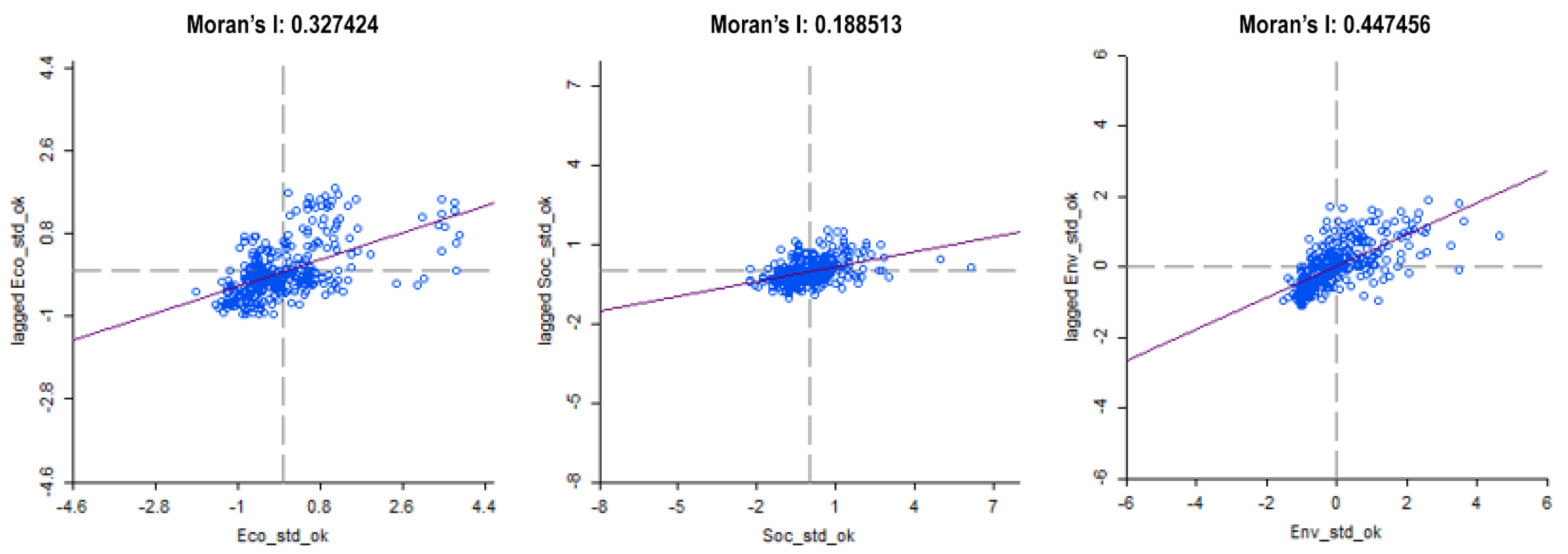
3.2. Local-Scale Spatial Interdependency of LSI

Figure 3 shows the Moran scatter plot and LISA cluster map for each LSI. The Moran scatters plot shows that the spatial autocorrelation value or global Moran index for LSIeco, LSIsoc, and LSIenv are 0.33, 0.18, and 0.45, respectively. It shows that all the LSI have a clustered pattern since the value is positive and more than 0. The result of the local Moran index may help to identify local spatial autocorrelation of LSI value in JBMUR. As for LSIeco, High-High (HH, high values surrounded by high values) category subdistricts are in Jakarta, Tangerang, Bekasi, and Depok (in the LISA cluster map, the HH subdistricts are shown in red). This pattern means that LSIeco is concentrated and clustered in the center area of Jabodetabek, or mainly in the subdistricts of Jakarta Province and its surrounding area.

As for LISA value of LSIsoc, HH category subdistricts are concentrated in the southern side of Cianjur Regency and in the northern side of Karawang Regency. Regarding LISA value of LSIenv, HH category subdistricts are concentrated in Cianjur Regency, the eastern side of Bogor Regency, the western side of Bandung, and Bandung Barat Regency. LL category subdistricts are concentrated in the Jakarta Province, Tangerang, Bekasi, and Depok. Most subdistricts in Jakarta Province with high LISA values of LSIeco, have low LISA values of LSIenv. These results aligned with Pravitasari et al. [49,80] which mentioned a trade-off between economy and environmental conditions in Jakarta Province and its surrounding area.

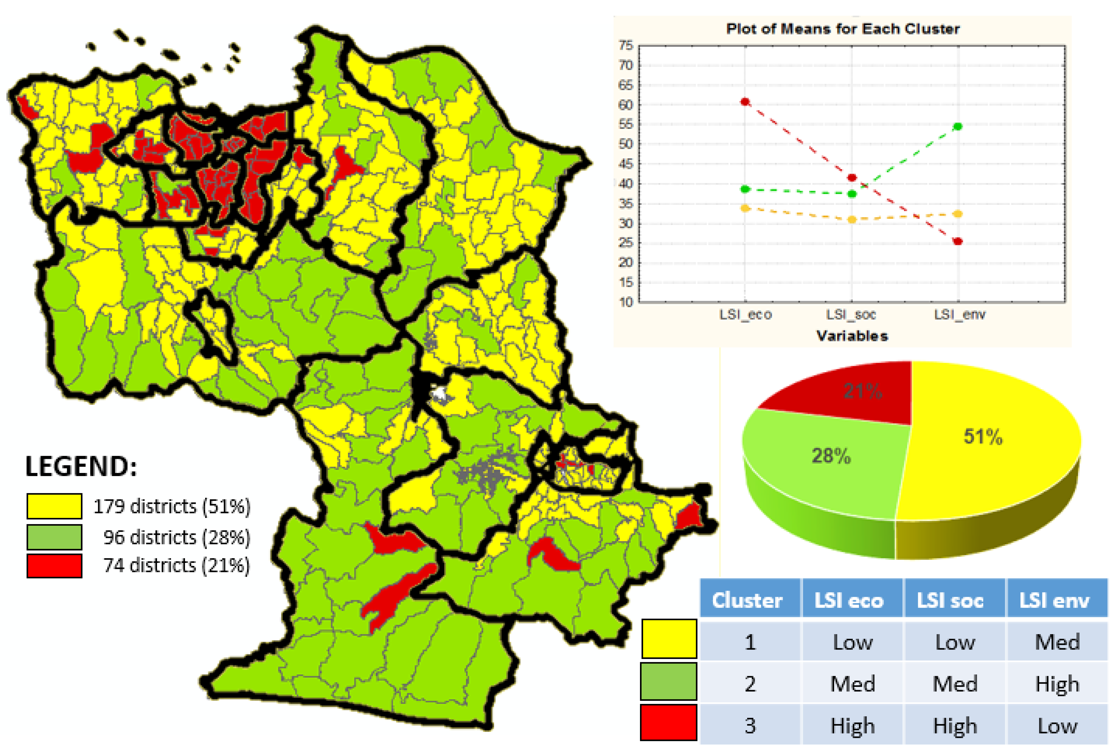
3.3. LSI-Based Clusters

The last result of this study is a cluster map of subdistricts based on the characteristics of local sustainability performance or LSI value (LSI₁, LSI₂, and LSI₃). According to the result, there are three clusters produced by the K-means clustering method. The distribution member of each cluster can be seen in Figure 4. There are 74 subdistricts (21%) categorized as cluster 3, and most of those subdistricts are in Jakarta Province. Their characteristics are high sustainability in the economy and social dimension but low in environmental dimension. This condition also occurs in other cities in the world [81,82]. There are 96 subdistricts (28%) categorized as cluster 2: moderate scores in economic and social dimension but high values in environmental dimension. Most subdistricts in JBMUR are categorized in cluster 1 (179 subdistricts or 51%), i.e., having low values in economy and social dimension but moderate value in environmental dimension. Subdistricts of Cluster 2 and Cluster 1 are scattered across JBMUR.

This study’s results strengthen the previous study’s conclusion, especially regarding the metropolitan core of Jakarta and Bandung in terms of their sustainability status [83,84,85]. Metropolitan cores, especially Jakarta and Bandung in our case tend to have low environmental sustainability and high economic sustainability. High economic sustainability in urban centers is driven by completeness of facilities and variety of sources of income. However, in general, JBMUR metropolitan centers often experience environmental problems such as floods. Therefore, metropolitan centers tend to have low environmental sustainability.

In Jakarta, the core of JBMUR, rapid urbanization has led to environmental degradation and food production [85,86,87]. Environmental degradation is marked by land subsidence, saltwater intrusion, polluted water sources, and air pollution [83,84]. Furthermore, several studies have also stated that Jakarta development has exceeded the carrying capacity [58,88], indicated by the frequent flooding, because the riverbank is used for settlements, and the lack of water catchment areas (limited green space) [85,89]. In social aspects, the continuing in-migration to Jakarta presents the problems such as slum areas, unemployment, crimes, and disparity [56]. However, regardless the inconvenience of social and environmental condition, metropolitan centers such as Jakarta remain attractive for migrants because they are vital economic centers and hubs in Indonesia, and even in Southeast Asia [90,91].

4. Conclusions

The local sustainability index (LSI) which was developed in this research can be used as indicators to promote sustainable development in JBMUR at the subdistrict level. By utilizing factor analysis, we could create a composite index of LSI for each dimension. Characteristic variables that make up the local sustainability index (LSI) in the economic dimension include factors of accessibility to economic facilities and infrastructure; accessibility to megacity cores; and high industrial activity. Characteristic variables that make up LSI in the social dimension include factors of accessibility to public facilities and health; public health conditions; poverty rates and access to employment; and population density. Meanwhile, the indicators that make up the LSI on the environmental dimension include the presence of green areas; disaster aspects; and the geographic physical characteristics of the region.

In general, subdistricts with high LSIeco are concentrated in subdistricts of Jakarta Province, and several subdistricts in Bandung City and its surroundings. However, high LSIeco values are generally not followed by a high LSIenv value. This phenomenon is found in most subdistricts in Jakarta Province, where this region has a very high percentage of built-up areas. On the other hand, some subdistricts in Bogor, Cianjur, and Bandung Regency have higher LSIenv values, where these regions have a moderate or low percentage of built-up area. As for LSIsoc values, there is no significant pattern found. A total of 77% of the subdistricts in JBMUR are categorized as having low LSIsoc values.

Spatial interdependency of local sustainability performance exists in subdistricts—the local-scale spatial units. The LSI in each subdistrict is strongly influenced by the sustainability condition of its surrounding areas. Then, based on the subdistrict clustering, most subdistricts in JBMUR are categorized in cluster 1 (179 subdistricts or 51% from the total number of subdistricts), which have low values in economy and the social dimension but moderate values in the environmental dimension. In addition, nearly all subdistricts of Jakarta Province (21% of the total number of subdistricts) are categorized in cluster 3, characterized by high values in the economic and social dimension but low values in environmental dimension.

The combination of LISA, LSI, and cluster analysis techniques in this study can capture a regional typology that highlight the characteristics of each region based on their sustainability condition. From the results of the cluster analysis, it can be seen that the sub-regions falling into the category of cluster 3 (red areas) are dominated by core megacity areas which have a high level of sustainability in the economic and social aspects, but their sustainability for the environmental dimension is low. Areas falling into the cluster 2 category (green area) are areas with rural characteristics that have a fairly good sustainability performance, especially seen from the value of the sustainability index for the environmental dimension. Meanwhile, the areas included in the cluster 1 category (yellow area) are areas with suburban characteristics and are areas in the JBMUR conurbation corridor. The areas in this cluster are the worst in terms of the conditions of sustainable development. They are dominant in number—51% of the total subdistricts in JBMUR. This shows that there are still many areas in suburban areas that have quite serious problems, especially in socio-economic aspects. Those problems are the poverty rate, which is still quite high, difficulties in terms of accessibility to economic facilities and infrastructure, access to public and health facilities, and access to the job market.

The results of this study further strengthen the tradeoff between socio-economic and environmental aspects. Areas with a high level of development tend to have a good development sustainability performance in the economic and social dimensions. On the contrary, their sustainability for the environmental dimension is low. The LSI as a composite index can be utilized to indicate locations of the sustainable state. Combined with cluster analysis, the LSI can identify typologies of subdistricts in JBMUR to capture the general sustainability state among subdistricts.

References

1. Emas, R. The Concept of Sustainable Development: Definition and Defining Principles. In United Nations’ 2015 Global Sustainable Development Report; United Nations: New York, NY, USA, 2015; pp. 1–3. [Google Scholar] [CrossRef]
2. Panayotou, T. Economic Growth and the Environment. In The Environment in Anthropology: A Reader in Ecology, Culture, and Sustainable Living; Haenn, N., Harnish, A., Wilk, R.R., Eds.; New York University Press: New York, NY, USA, 2020; pp. 140–148. [Google Scholar] [CrossRef]
3. Klarin, T. The Concept of Sustainable Development: From Its Beginning to the Contemporary Issues. Zagreb Int. Rev. Econ. Bus. 2018, 21, 67–94. [Google Scholar] [CrossRef] [Green Version]
4. Schilling, M.; Chiang, L. The Effect of Natural Resources on a Sustainable Development Policy: The Approach of Non-Sustainable Externalities. Energy Policy 2011, 39, 990–998. [Google Scholar] [CrossRef]
5. Dernbach, J.C. Sustainable Development as a Framework for National Governance. Case West. Reserve. Law Rev. 1998, 2011, 49. [Google Scholar]
6. Holden, E.; Linnerud, K.; Banister, D. Sustainable Development: Our Common Future Revisited. Glob. Environ. Change 2014, 26, 130–139. [Google Scholar] [CrossRef] [Green Version]
7. Borowy, I. Defining Sustainable Development for Our Common Future: A History of the World Commission on Environment and Development (Brundtland Commission), 1st ed.; Routledge Taylor and Francis: New York, NY, USA, 2013. [Google Scholar] [CrossRef]
8. Wall, G. Beyond Sustainable Development. Tour. Recreat. Res. 2018, 43, 390–399. [Google Scholar] [CrossRef]
9. United Nations. Report of World Commission on Environment and Development: Our Common Future; United Nations: New York, NY, USA, 1987. [Google Scholar]
10. Schaltegger, S.; Hansen, E.G.; Lüdeke-Freund, F. Business Models for Sustainability: Origins, Present Research, and Future Avenues. Organ Environ. 2015, 29, 3–10. [Google Scholar] [CrossRef]
11. Morelli, J. Environmental Sustainability: A Definition for Environmental Professionals. J. Environ. Sustain. 2013, 1, 2. [Google Scholar] [CrossRef] [Green Version]
12. Purvis, B.; Mao, Y.; Robinson, D. Three Pillars of Sustainability: In Search of Conceptual Origins. Sustain. Sci. 2018, 14, 681–695. [Google Scholar] [CrossRef]
13. Hansmann, R.; Mieg, H.A.; Frischknecht, P. Principal Sustainability Components: Empirical Analysis of Synergies between the Three Pillars of Sustainability. Int. J. Sustain. Dev. World Energy 2012, 19, 451–459. [Google Scholar] [CrossRef]
14. Moldan, B.; Janoušková, S.; Hák, T. How to Understand and Measure Environmental Sustainability: Indicators and Targets. Ecol. Indic. 2012, 17, 4–13. [Google Scholar] [CrossRef]
15. Mensah, J. Sustainable Development: Meaning, History, Principles, Pillars, and Implications for Human Action: Literature Review. Cogent. Soc. Sci. 2019, 5, 1–21. [Google Scholar] [CrossRef]
16. Asara, V.; Otero, I.; Demaria, F.; Corbera, E. Socially Sustainable Degrowth as a Social–Ecological Transformation: Repoliticizing Sustainability. Sustain. Sci. 2015, 10, 375–384. [Google Scholar] [CrossRef] [Green Version]
17. Choi, H.C.; Turk, E.S. Sustainability Indicators for Managing Community Tourism. In Quality-of-Life Community Indicators for Parks, Recreation and Tourism Management; Budruk, M., Phillips, R., Eds.; Springer: Dordrecht, Germany, 2011; pp. 115–140. [Google Scholar] [CrossRef]
18. Elkington, J. Cannibals with Forks: The Triple Bottom Line of 21st Century Business; John Wiley & Son: Hoboken, NJ, USA, 1999. [Google Scholar]
19. Bell, S.; Morse, S. Sustainability Indicators Past and Present: What Next? Sustainability 2018, 10, 1688. [Google Scholar] [CrossRef] [Green Version]
20. Böhringer, C.; Jochem, P.E.P.P. Measuring the Immeasurable—A Survey of Sustainability Indices. Ecol. Econ. 2007, 63, 1–8. [Google Scholar] [CrossRef] [Green Version]
21. Ramos, T.; Pires, S.M. Sustainability Assessment: The Role of Indicators. In Sustainability Assessment Tools in Higher Education Institutions: Mapping Trends and Good Practices Around the World; Caeiro, S., Filho, W.L., Jabbour, C., Azeiteiro, U.M., Eds.; Springer: Cham, Switzerland, 2013; pp. 81–99. [Google Scholar] [CrossRef]
22. Ahi, P.; Searcy, C.; Jaber, M.Y. A Quantitative Approach for Assessing Sustainability Performance of Corporations. Ecol. Econ. 2018, 152, 336–346. [Google Scholar] [CrossRef]
23. Shokravi, S.; Kurnia, S. A Step towards Developing a Sustainability Performance Measure within Industrial Networks. Sustainability 2014, 6, 2201–2222. [Google Scholar] [CrossRef]
24. Jha, M.K.; Ogallo, H.G.; Owolabi, O. A Quantitative Analysis of Sustainability and Green Transportation Initiatives in Highway Design and Maintenance. Procedia Soc. Behav. Sci. 2014, 111, 1185–1194. [Google Scholar] [CrossRef] [Green Version]
25. Dahl, A.L. Achievements and Gaps in Indicators for Sustainability. Ecol. Indic. 2012, 17, 14–19. [Google Scholar] [CrossRef]
26. Shen, L.; Wu, Y.; Zhang, X. Key Assessment Indicators for the Sustainability of Infrastructure Projects. J. Constr. Eng. Manag. 2010, 137, 441–451. [Google Scholar] [CrossRef] [Green Version]
27. Tippett, N.; Wolke, D. Socioeconomic Status and Bullying: A Meta-Analysis. Am. J. Public Health 2014, 104, e48–e49. [Google Scholar] [CrossRef]
28. Hák, T.; Janoušková, S.; Moldan, B. Sustainable Development Goals: A Need for Relevant Indicators. Ecol. Indic. 2016, 60, 565–573. [Google Scholar] [CrossRef]
29. Chaudhary, A.; Gustafson, D.; Mathys, A. Multi-Indicator Sustainability Assessment of Global Food Systems. Nat. Commun. 2018, 9, 848. [Google Scholar] [CrossRef] [Green Version]
30. Kennedy, C.; Stewart, I.D.; Ibrahim, N.; Facchini, A.; Mele, R. Developing a Multi-Layered Indicator Set for Urban Metabolism Studies in Megacities. Ecol. Indic. 2014, 47, 7–15. [Google Scholar] [CrossRef]
31. Albertí, J.; Balaguera, A.; Brodhag, C.; Fullana-i-Palmer, P. Towards Life Cycle Sustainability Assessment of Cities. A Review of Background Knowledge. Sci. Total Environ. 2017, 609, 1049–1063. [Google Scholar] [CrossRef]
32. Ciegis, R.; Ramanauskiene, J.; Startiene, G. Theoretical Reasoning of the Use of Indicators and Indices for Sustainable Development Assessment. Eng. Econ. 2009, 63, 33–40. [Google Scholar]
33. Singh, R.K.; Murty, H.R.; Gupta, S.K.; Dikshit, A.K. An Overview of Sustainability Assessment Methodologies. Ecol. Indic. 2012, 15, 281–299. [Google Scholar] [CrossRef]
34. Cook, D.; Saviolidis, N.M.; Davíðsdóttir, B.; Jóhannsdóttir, L.; Ólafsson, S. Measuring Countries’ Environmental Sustainability Performance—The Development of a Nation-Specific Indicator Set. Ecol. Indic. 2017, 74, 463–478. [Google Scholar] [CrossRef]
35. Wilson, M.C.; Wu, J. The Problems of Weak Sustainability and Associated Indicators. Int. J. Sustain. Dev. World Ecol. 2017, 24, 44–51. [Google Scholar] [CrossRef]
36. Parris, T.M.; Kates, R.W. Characterizing and Measuring Sustainable Development. Annu. Rev. Environ. Resour. 2003, 28, 559–586. [Google Scholar] [CrossRef]
37. Pacione, M. Urban Environmental Quality and Human Wellbeing—A Social Geographical Perspective. Landsc. Urban Plan 2003, 65, 19–30. [Google Scholar] [CrossRef]
38. Van Kamp, I.; Leidelmeijer, K.; Marsman, G.; De Hollander, A. Urban Environmental Quality and Human Well-Being: Towards a Conceptual Framework and Demarcation of Concepts; a Literature Study. Landsc. Urban Plan 2003, 65, 5–18. [Google Scholar] [CrossRef]
39. Waas, T.; Hugé, J.; Block, T.; Wright, T.; Benitez-Capistros, F.; Verbruggen, A. Sustainability Assessment and Indicators: Tools in a Decision-Making Strategy for Sustainable Development. Sustainability 2014, 6, 5512–5534. [Google Scholar] [CrossRef] [Green Version]
40. Mayer, A.L. Strengths and Weaknesses of Common Sustainability Indices for Multidimensional Systems. Environ. Int. 2008, 34, 277–291. [Google Scholar] [CrossRef] [PubMed]
41. Wu, J.; Wu, T. Sustainability Indicators and Indices: An Overview. In Handbook of Sustainability Management; Madu, C.N., Kuei, C.-H., Eds.; World Scientific: Singapore, 2012; pp. 65–86. [Google Scholar] [CrossRef]
42. Kwatra, S.; Kumar, A.; Sharma, P. A Critical Review of Studies Related to Construction and Computation of Sustainable Development Indices. Ecol. Indic. 2020, 112, 106061. [Google Scholar] [CrossRef]
43. Moldan, B.; Dahl, A.L. Challenges to Sustainability Indicators. In Sustainability Indicators A Scientific Assessment; Hák, T., Moldan, B., Dahl, A.L., Eds.; Island Press: Washington, DC, USA, 2007. [Google Scholar]
44. Winograd, M.; Farrow, A. Sustainable Development Indicators for Decision Making: Concepts, Methods, Definition and Use. In Dimensions of Sustainable Development; Bawa, K.S., Seidler, R., Eds.; Eolss Publishers: Oxford, UK, 2007; Volume 1, pp. 41–73. [Google Scholar]
45. Evans, B.; Joas, M.; Sundback, S.; Theobald, K. Governing Sustainable Cities, 1st ed.; Routledge: London, UK, 2013. [Google Scholar] [CrossRef]
46. Coenen, L.; Benneworth, P.; Truffer, B. Toward a Spatial Perspective on Sustainability Transitions. Res. Policy 2012, 41, 968–979. [Google Scholar] [CrossRef]
47. Berardi, U. Sustainability Assessment of Urban Communities through Rating Systems. Environ. Dev. Sustain. 2013, 15, 1573–1591. [Google Scholar] [CrossRef]
48. Rama, M.; González-García, S.; Andrade, E.; Moreira, M.T.; Feijoo, G. Assessing the Sustainability Dimension at Local Scale: Case Study of Spanish Cities. Ecol. Indic. 2020, 117, 106687. [Google Scholar] [CrossRef]
49. Pravitasari, A.E.; Saizen, I.; Rustiadi, E. Towards Resilience of Jabodetabek Megacity: Developing Local Sustainability Index with Considering Local Spatial Interdependency. Int. J. Sustain. Future Human Secur. 2016, 4, 27–34. [Google Scholar] [CrossRef]
50. Pravitasari, A.E.; Rustiadi, E.; Singer, J.; Fuadina, L.N. Developing Local Sustainability Index (LSI) at Village Level in Jambi Province. In International Proceeding of the 8th Rural Research and Planning Group International Conference, Yogyakarta, Indonesia, 17–18 May 2017; Suratman, Baiquni, M., Hasanati, S., Eds.; Gadjah Mada University Press: Yogyakarta, Indonesia, 2018; pp. 15–29. [Google Scholar]
51. Yudha, E.P.; Juanda, B.; Kolopaking, L.M.; Kinseng, R.A. Rural Development Policy and Strategy in the Rural Autonomy Era. Case Study of Pandeglang Regency-Indonesia. Hum. Geogr. 2020, 14, 125–147. [Google Scholar] [CrossRef]
52. Statistics Indonesia. Luas daerah dan jumlah pulau menurut Provinsi 2002–2016. 9 February. Available online: https://www.bps.go.id/statictable/2014/09/05/1366/luas-daerah-dan-jumlah-pulau-menurut-provinsi-2002-2016.html (accessed on 9 February 2020).
53. Statistics Indonesia. Statistical Yearbook of Indonesia 2022; Statistics Indonesia: Jakarta, Indonesia, 2022. [Google Scholar]
54. Buchori, I.; Sugiri, A.; Maryono, M.; Pramitasari, A.; Pamungkas, I.T.D. Theorizing Spatial Dynamics of Metropolitan Regions: A Preliminary Study in Java and Madura Islands, Indonesia. Sustain. Cities Soc. 2017, 35, 468–482. [Google Scholar] [CrossRef]
55. Bakri, B.; Rustiadi, E.; Fauzi, A.; Adiwibowo, S. Regional Sustainable Development Indicators for Developing Countries: Case Study of Provinces in Indonesia. Int. J. Sustain. Dev. 2018, 21, 102–130. [Google Scholar] [CrossRef]
56. Rustiadi, E.; Pribadi, D.O.; Pravitasari, A.E.; Indraprahasta, G.S.; Iman, L.S. Jabodetabek Megacity: From City Development toward Urban Complex Management System. In Urban Development Challenges, Risks and Resilience in Asian Mega Cities; Singh, R.B., Ed.; Springer: Tokyo, Japan, 2015; pp. 421–445. [Google Scholar] [CrossRef]
57. Pravitasari, A.E.; Rustiadi, E.; Priatama, R.A.; Murtadho, A.; Kurnia, A.A.; Mulya, S.P.; Saizen, I.; Widodo, C.E.; Wulandari, S. Spatiotemporal Distribution Patterns and Local Driving Factors of Regional Development in Java. ISPRS Int. J. Geoinf. 2021, 10, 812. [Google Scholar] [CrossRef]
58. Pravitasari, A.E.; Rustiadi, E.; Mulya, S.P.; Widodo, C.E.; Indraprahasta, G.S.; Fuadina, L.N.; Karyati, N.E.; Murtadho, A. Measuring Urban and Regional Sustainability Performance in Java: A Comparison Study between 6 Metropolitan Areas. IOP Conf. Ser. Earth Environ. Sci. 2020, 556, 012004. [Google Scholar] [CrossRef]
59. Rustiadi, E.; Pravitasari, A.E.; Setiawan, Y.; Mulya, S.P.; Pribadi, D.O.; Tsutsumida, N. Impact of Continuous Jakarta Megacity Urban Expansion on the Formation of the Jakarta-Bandung Conurbation over the Rice Farm Regions. Cities 2021, 111, 103000. [Google Scholar] [CrossRef]
60. Fernando, M.A.C.S.S.; Samita, S.; Abeynayake, R. Modified Factor Analysis to Construct Composite Indices: Illustration on Urbanization Index. Trop. Agric. Res. 2012, 23, 337. [Google Scholar] [CrossRef]
61. Mattjik, A.A.; Sumertajaya, I.M. Sidik Peubah Ganda Dengan Menggunakan SAS; Wibawa, G.N.A., Hadi, A.F., Eds.; IPB Press: Bogor, Indonesia, 2011. [Google Scholar]
62. Morey, L.C.; Blashfield, R.K.; Skinner, H.A. A Comparison of Cluster Analysis Techniques Withing a Sequential Validation Framework. Multivar. Behav. Res. 1983, 18, 309–329. [Google Scholar] [CrossRef]
63. Priatama, R.A.; Rustiadi, E.; Widiatmaka, W.; Pravitasari, A.E. Physical Geographical Factors Leading to the Disparity of Regional Development: The Case Study of Java Island. Indones. J. Geogr. 2022, 54, 195–205. [Google Scholar] [CrossRef]
64. Babu, S.C.; Gajanan, S.N. Classifying Households on Food Security and Poverty Dimensions—Application of K-Means Cluster Analysis. In Food Security, Poverty and Nutrition Policy Analysis; Academic Press: Cambridge, MA, USA, 2022; pp. 493–526. [Google Scholar] [CrossRef]
65. Bogdanov, N.; Meredith, D.; Efstratoglou, S. A Typology of Rural Areas in Serbia. Econ. Ann. 2008, 53, 7–29. [Google Scholar] [CrossRef]
66. Topaloglou, L.; Kallioras, D.; Manetos, P.; Petrakos, G. A Border Regions Typology in the Enlarged European Union. J. Bord. Stud. 2011, 20, 67–89. [Google Scholar] [CrossRef]
67. Budiyantini, Y.; Pratiwi, V. Peri-Urban Typology of Bandung Metropolitan Area. Procedia Soc. Behav. Sci. 2016, 227, 833–837. [Google Scholar] [CrossRef] [Green Version]
68. Firoz, M.C.; Banerji, H.; Sen, J. A Methodology to Define the Typology of Rural Urban Continuum Settlements in Kerala. J. Reg. Dev. Plan. 2014, 3, 49–60. [Google Scholar]
69. Pacini, G.C.; Colucci, D.; Baudron, F.; Righi, E.; Corbeels, M.; Tittonell, P.; Stefanini, F.M. Combining Multi-Dimensional Scaling and Cluster Analysis to Describe the Diversity of Rural Households. Exp. Agric. 2014, 50, 376–397. [Google Scholar] [CrossRef] [Green Version]
70. Ballas, D.; Kalogeresis, T.; Labriandis, L. A Comparative Study of Typologies for Rural Areas in Europe. In Proceedings of the 43rd European Congress of the Regional Science Association, Jyväskylä, Finland, 27–30 August 2003; Regional Science Association: Jyväskylä, Finland, 2003; pp. 1–38. [Google Scholar]
71. Krehl, A.; Siedentop, S. Towards a Typology of Urban Centers and Subcenters—Evidence from German City Regions. Urban Geogr. 2019, 40, 58–82. [Google Scholar] [CrossRef] [Green Version]
72. Kozonogova, E.; Dubrovskaya, J. The Method of Regions’ Typology by the Level of Cluster Potential. In Eurasian Ecoomic Perspectives; Bilgin, M.H., Danis, H., Demir, E., Can, U., Eds.; Springer: Cham, Switzerland, 2019; Volume 10, pp. 195–205. [Google Scholar] [CrossRef]
73. Kladivo, P.; Ptáček, P.; Roubínek, P.; Ziener, K. The Czech-Polish and Austrian-Slovenian Borderland–Similarities and Differences of Development and Typology of Regions. Morav. Geograph. Rep. 2012, 20, 22–37. [Google Scholar]
74. Saputra, D.M.; Saputra, D.; Oswari, L.D. Effect of Distance Metrics in Determining K-Value in K-Means Clustering Using Elbow and Silhouette Method. In Proceedings of the Sriwijaya International Conference on Information Technology and Its Applications (SICONIAN 2019), Palembang, Indonesia, 16 November 2019; Volume 172, pp. 341–346. [Google Scholar] [CrossRef]
75. Zhou, P.; Ang, B.W. Indicators for Assessing Sustainability Performance. In Handbook of Performability Engineering; Misra, K.B., Ed.; Springer: London, UK, 2008; pp. 905–918. [Google Scholar] [CrossRef]
76. Kline, R. Exploratory and Confirmatory Factor Analysis. In Applied Quantitative Analysis in Education and the Social Sciences; Petscher, Y., Schatschneider, C., Compton, D.L., Eds.; Taylor and Francis: New York, NW, USA, 2013; pp. 1–376. [Google Scholar] [CrossRef]
77. Kline, P. An Easy Guide to Factor Analysis, 1st ed.; Routledge: London, UK, 2014. [Google Scholar] [CrossRef]
78. Gorsuch, R.L. Factor Analysis, 2nd ed.; Routledge: London, UK, 2014. [Google Scholar]
79. Yong, A.G.; Pearce, S. A Beginner’s Guide to Factor Analysis: Focusing on Exploratory Factor Analysis. Tutor Quant. Methods Psychol. 2013, 9, 79–94. [Google Scholar] [CrossRef] [Green Version]
80. Pravitasari, A.E.; Rustiadi, E.; Mulya, S.P.; Setiawan, Y.; Fuadina, L.N.; Murtadho, A. Identifying the Driving Forces of Urban Expansion and Its Environmental Impact in Jakarta-Bandung Mega Urban Region. IOP Conf. Ser. Earth Environ. Sci. 2018, 149, 012044. [Google Scholar] [CrossRef] [Green Version]
81. Basiago, A.D. Economic, Social, and Environmental Sustainability in Development Theory and Urban Planning Practice. Environmentalist 1998, 19, 145–161. [Google Scholar] [CrossRef]
82. González-García, S.; Rama, M.; Cortés, A.; García-Guaita, F.; Núñez, A.; Louro, L.G.; Moreira, M.T.; Feijoo, G. Embedding Environmental, Economic and Social Indicators in the Evaluation of the Sustainability of the Municipalities of Galicia (Northwest of Spain). J. Clean. Prod. 2019, 234, 27–42. [Google Scholar] [CrossRef]
83. Cao, A.; Esteban, M.; Valenzuela, V.P.B.; Onuki, M.; Takagi, H.; Thao, N.D.; Tsuchiya, N. Future of Asian Deltaic Megacities under Sea Level Rise and Land Subsidence: Current Adaptation Pathways for Tokyo, Jakarta, Manila, and Ho Chi Minh City. Curr. Opin. Environ. Sustain. 2021, 50, 87–97. [Google Scholar] [CrossRef]
84. Henny, C.; Meutia, A.A. Urban Lakes in Megacity Jakarta: Risk and Management Plan for Future Sustainability. Procedia Environ. Sci. 2014, 20, 737–746. [Google Scholar] [CrossRef]
85. Pribadi, D.O.; Vollmer, D.; Pauleit, S. Impact of Peri-Urban Agriculture on Runoff and Soil Erosion in the Rapidly Developing Metropolitan Area of Jakarta, Indonesia. Reg. Environ. Chang. 2018, 18, 2129–2143. [Google Scholar] [CrossRef]
86. Indraprahasta, G.S. The Potential of Urban Agriculture Development in Jakarta. Procedia Environ. Sci. 2013, 17, 11–19. [Google Scholar] [CrossRef] [Green Version]
87. Pribadi, D.O.; Pauleit, S. The Dynamics of Peri-Urban Agriculture during Rapid Urbanization of Jabodetabek Metropolitan Area. Land Use Policy 2015, 48, 13–24. [Google Scholar] [CrossRef]
88. Hudalah, D.; Firman, T. Beyond Property: Industrial Estates and Post-Suburban Transformation in Jakarta Metropolitan Region. Cities 2012, 29, 40–48. [Google Scholar] [CrossRef]
89. Maheng, D.; Pathirana, A.; Zevenbergen, C. A Preliminary Study on the Impact of Landscape Pattern Changes Due to Urbanization: Case Study of Jakarta, Indonesia. Land 2021, 10, 218. [Google Scholar] [CrossRef]
90. Indraprahasta, G.S.; Derudder, B. World City-Ness in a Historical Perspective: Probing the Long-Term Evolution of the Jakarta Metropolitan Area. Habitat. Int. 2019, 89, 102000. [Google Scholar] [CrossRef]
91. Kurnia, A.A.; Rustiadi, E.; Pravitasari, A.E. Characterizing Industrial-Dominated Suburban Formation Using Quantitative Zoning Method: The Case of Bekasi Regency, Indonesia. Sustainability 2020, 12, 8094. [Google Scholar] [CrossRef]
Figure 1. The administration map of the JBMUR.
Sustainability 14 13913 g001
Figure 2. Spatial distribution of the local sustainability index (LSI): economy, social, and environment.
Sustainability 14 13913 g002
Figure 3. Global and local Moran’s index (LISA) for LSI economy, social, and environment and its statistical significance values.
Sustainability 14 13913 g003aSustainability 14 13913 g003bSustainability 14 13913 g003c
Figure 4. Typology of subdistricts in JBMUR based on the characteristics of LSI.
Sustainability 14 13913 g004