Article

Response of Water Yield to Future Climate Change Based on InVEST and CMIP6—A Case Study of the Chaohu Lake Basin

1
School of Environment and Energy Engineering, Anhui Jianzhu University, Hefei 230601, China
2
Institute of Remote Sensing and Geographic Information System, Anhui Jianzhu University, Hefei 230601, China
*
Author to whom correspondence should be addressed.
Sustainability 2022, 14(21), 14080; https://doi.org/10.3390/su142114080
Submission received: 3 October 2022 / Revised: 24 October 2022 / Accepted: 24 October 2022 / Published: 28 October 2022
(This article belongs to the Special Issue Climate Change, Land Use Change and Water Resources)

Abstract

:
The Chaohu Lake Basin (CLB) is the main flow area of the Yangtze River–Huaihe River Water Transfer Project in Central China. It is important to quantitatively evaluate the water resources in the CLB and predict their response to future climate change. This study simulated and calibrated the water yield in the CLB from 2000 to 2019 based on InVEST. We also analyzed the influence factor on the water yield and predicted the water yield in future years with CMIP6 data. The results demonstrate that: (1) The InVEST water production module had good applicability in this study region. There was a strong linear relationship between the simulated water yield and the observed surface runoff (y = 1.2363x − 8.6038, R2 = 0.868, p < 0.01); (2) The explanatory percentage of interaction between precipitation and land use/land cover for water yield in 2001, 2008, and 2016 reached 71%, 77%, and 85%, respectively, which were the two dominant factors affecting water yield in the CLB; and (3) The average annual water yield in the CLB increased under the SSP2-4.5, SSP3-7.0, and SSP5-8.5 future scenarios with increasing precipitation, increased with 71%, 139.8%, and 159.5% in 2100 compared with 2040, respectively. The overall trend of water production decreased with increases in carbon emission intensity.

1. Introduction

Ecosystems provide freshwater resources for humans and are important for maintaining regional ecosystem functions, populations, and socioeconomic development [1,2]. They provide basic support for regional water resource management and planning [3]. With global climate change, population growth, and land use/land cover(LULC) changes due to human activities, water scarcity and water environment pollution problems are becoming increasingly prominent [4]. The degradation of ecosystem services is seriously troubling for human survival and development [5,6]. Climate change directly affects regional rainfall and evapotranspiration, which further affect the water cycle and vegetation growth status [7]. It will play an important role in the global water cycle and water resource effectiveness in the coming decades. It is a cutting-edge and topical issue to evaluate ecosystem water supply capacity in a spatio-temporal way and its response to climate change and human activities in current hydrology and ecology research. Chaohu Lake is located on the left bank of the lower Yangtze River in East China. It is one of the five major freshwater lakes in China. It provides water for industrial and agricultural activities. Additionally, it is the crucial habitat of migratory birds between the Yangtze River and the Huaihe River. Chaohu Lake Basin (CLB) is an important part of Hefei’s urban ecosystem, which is the largest city near Chaohu Lake and a rapidly developing capital city of Anhui Province with a permanent population of nearly 10 million. The CLB is the main flow area of the Yangtze River–Huaihe River Water Transfer Project (YHWTP). The quantitative evaluation and prediction of water resources in the CLB are significant to water resource allocation, optimal dispatching of YHWTP, and ecological environmental management in the region.
The evaluation of ecosystem water supply function requires understanding the regional ecosystem’s structure and major processes. This process mainly adopts the establishment of ecosystem service assessment and optimization model systems to elucidate the formation and interaction mechanisms of ecosystem water supply services [8,9]. The model systems include service tradeoffs, change analysis, and scenario prediction [10,11]. In recent years, many scholars have started to conduct watershed water resource evaluation by establishing models including hydrological models such as the Soil and Water Assessment (SWAT) [12,13], MIKE SHE [14,15], SCS-CN [16,17], and special models for ecosystem services such as Integrated Valuation of Ecosystem Services and Tradeoffs (InVEST) [18], etc. It has been verified that the SWAT model has obvious advantages at the seasonal and monthly scales, and the InVEST model is more suitable than the SWAT model in assessing the water content at the annual scale [19]. The SWAT model required a larger number of expert skills for the detailed hydrological processes, and it also took longer to run the model because of the complicated input data. The InVEST model required a smaller amount of input data for a simplified hydrological process, which made it easier to be implemented [20]. The InVEST model is a comprehensive model for quantifying and valuing ecosystem services. It has been applied in the Americas, Africa, and the Yangtze River Basin in China, and it has achieved good simulation results [21,22,23,24,25]. It is based on a GIS platform and uses a simplified hydrological model for the evaluation of ecosystem services. The model was not developed to reproduce empirical observations [26]. It features quantitative ecosystem service functions in the form of maps and facilitates the use of assessment results for planning, management, and scenario prediction [27]. Studies by scholars have focused on localized applications of the InVEST model [28,29], including parameter sensitivity analysis [30,31], dynamic assessment of ecosystem services [32], and comparative studies with other hydrological models [20,33].
Based on the ecosystem services framework, prediction analysis of future climate change on regional water resources and water supply capacity is rare. There are only a few cases. Yang et al. evaluated the impact of future climate change on water supply in a typical East Asian monsoon basin in South China by coupling the InVEST model and the statistical downscaling technique model (SDSM), and the results demonstrated an increasing trend in annual average precipitation and reference evapotranspiration. In particular, the average annual water yield will increase by 19.3% (33.5%) in the future (2080–2095) under the RCP2.6 (4.5) scenario [34]. Yan et al. used the nutrient transport (NDR) module of the InVEST model to quantify the historical state of nonpoint-source nitrogen export in the Jiulong River Basin in southern China and constructed scenarios using artificial wetlands to predict the amount of change in nonpoint-source nitrogen export from the Jiulong River Basin under different land use and climate change scenarios [35].
The above studies assessed the impact of future climate change on regional water production and quality using the Fifth Coupled Model Comparison Program (CMIP5), a multi-climate model ensemble that averages results, coupled with InVEST water production and nutrient retention models. Few studies have used the Coupled Model Intercomparison Project Phase 6 (CMIP6) to predict water production, and model results have rarely been validated using measured data. Compared to CMIP5, CMIP6 considers more complex processes, and many models can bidirectionally couple atmospheric and chemical processes [36]. In addition, the RCP scenarios of CMIP5 only consider the goal of achieving stable CO2 concentrations and corresponding radiative forcing in the next 100 years [37]. It does not target a specific social development pathway, while the new shared socio-economic pathway of CMIP6 fully takes this into account, providing more diverse emission scenarios, which can provide more reasonable simulation results for mitigation adaptation studies and regional climate prediction [38,39].
Therefore, the research work of this paper focused on the following points. Firstly, we simulated the spatio-temporal variation of water yield in the CLB in the past 20 years by using measured basic data, such as hydrology, meteorology, and land use, and verified the reliability of the model in this study region with measured statistical data. Secondly, we elucidated the relationship between annual water yield and geographical factors in different hydrological years. Lastly, we predicted the spatio-temporal variation trend of future water yield in the CLB based on CMIP6 climatological model data. The results of this study will provide further insights into the potential impacts of climate change on the water supply capacity of ecosystems in the future and provide a basis for decision making regarding water resource management.

2. Materials and Methods

2.1. Study Region

The Chaohu Lake Basin (CLB) is located between the lower reaches of the Yangtze River and the Huai River Basin in the Anhui Province of East China (Figure 1). It ranges between 30°58′00″–32°58′00″ N and 116°24′30″–118°30′00″ E, covering an area of 14,203 km2 [40]. Chaohu Lake is one of the five largest freshwater lakes in China. The CLB consists of the five cities of Hefei, Wuhu, Maanshan, Tongling, and Luan. The topography of the basin is generally long from east to west, narrow from north to south, high in the west, and low in the east, with low-lying plains in the middle. The region has rich water resources. The 33 drainage rivers mainly come from the Dabieshan Mountains, flow from west to east radially through Chaohu Lake, and then flow together into the Yangtze River through the Yuxi River.
The CLB has a subtropical humid monsoon climate. The average temperature is 16 °C, the highest temperature is 41.3 °C, and the lowest temperature is minus 15.7 °C. The relative humidity of the CLB is 76%. The flood season is usually from May to August, and the average annual rainfall is about 1100 mm [41].
The study region is greatly affected by strong human disturbance. It is a key development and ecological protection zone in China. It is representative and typical to study water yield under the influence of climate change and rapid economic and social development.

2.2. Data

2.2.1. Model Operation Data

The data required for the water yield simulation model include: annual precipitation, annual reference evapotranspiration, land use/land cover map, plant available water content, root-restricting layer depth, watershed and sub-watersheds boundaries. The source descriptions of the above data are shown in Table 1.
Daily precipitation observations from 13 meteorological stations (Figure 1) in and around the study region from 2000 to 2019 were derived from the daily dataset of Chinese terrestrial climate information (V3.0), National Meteorological Science Data Center (NMSDC). All the observations were quality-controlled, and the data were preprocessed using ArcMap (v10.8) before model calculation to meet the data format requirements of the InVEST model, including inverse distance weight interpolation, projection, resampling, and mask extraction. Annual reference evapotranspiration was calculated using the FAO Penman–Monteith equation. It was defined as a hypothetical reference crop canopy evapotranspiration rate assuming a crop height of 0.12 m, a fixed surface resistance of 70 m/s for the crop, and an albedo of 0.23 [42]. The modified FAO Penman–Monteith expression is as follows.
PE = 0 . 408 Δ ( R n G ) + γ 900 T m e a n + 273 u 2 ( e s e a ) Δ + r ( 1 + 0 . 34 u 2 )
In the formula, PE represents reference evapotranspiration (mm/d), Δ represents the slope of saturated water pressure curve (kPa/°C), R n represents surface net radiation fluxes (MJ/(m·d)), G represents soil heat flux (MJ/(m2·d)), γ represents the wet and dry meter constant (kPa/°C), T mean represents mean daily temperature (°C), u 2 represents wind speed at 2 m high (m/s),   e s represents saturated water pressure (kPa), e a represents actual water pressure (kPa).
The daily observation data used in the above equation were also obtained from the daily dataset of Chinese terrestrial climate information (V3.0), National Meteorological Science Data Center (NMSDC). The parameters include the average temperature, maximum temperature, minimum temperature, relative humidity, sunshine hours, average air pressure, and average wind speed from 13 meteorological stations in and around the study region from 2000 to 2019. The annual reference evapotranspiration raster was preprocessed with the same process as the annual precipitation.
LULC rasters for 2000, 2005, 2010, 2015, and 2018 were obtained from the Resource and Environment Science and Data Center. The datasets were based on Landsat remote sensing images with a spatial resolution of 30 m × 30 m and generated through manual visual interpretation. The LULC map adopts a two-level classification system, as shown in Table 2. When the land use raster of one year was not available, we utilized the LULC in the year closest in time to the above five years. That is, the LULC for 2000, 2005, 2010, 2015, and 2018 were respectively taken to estimate water yields for 2000–2002, 2003–2007, 2008–2012, 2012–2016, and 2017–2019.
The root-restricting layer depth of the soil was obtained from the Harmonized World Soil Database (v1.2) with a spatial resolution of 1 km × 1 km. The plant available water content can be calculated by referring to the formula for estimating the effective water content of Chinese soils [43] in Equation (2).
ASWC = 54 . 509 0 . 132 sand % 0 . 003 sand % 2 0 . 055 silt % 0 . 006 silt % 2 0 . 738 clay % + 0 . 007 clay % 2 2 . 688 OM % + 0 . 501 OM % 2
In the formula, sand % , silt % , clay % , OM % represent contents of measured sand, silt, clay, and organic matter, respectively.

2.2.2. Model Validation Data

The observed annual surface runoff (m3) of the CLB was obtained from the Anhui Statistical Yearbook on the Anhui Provincial Bureau of Statistics website (http://tjj.ah.gov.cn/ (accessed on 15 April 2022)). The statistics of natural, annual surface runoff were converted to watershed units by administrative areas via the face interpolation method.

2.2.3. Factors Data

The driving factors included elevation, slope, aspect, annual vegetation index (NDVI), LULC, precipitation, reference evapotranspiration (RET), and hydrologic soil group (HSG). DEM data (30 m × 30 m) were obtained from the Lake-Watershed Science SubCenter, National Earth System Science Data Center, National Science & Technology Infrastructure of China. NDVI datasets were obtained from the Resource and Environment Science and Data Center at a 1 km spatial scale, which is the maximum value of monthly NDVI values from January to December of each year. The classification of hydrological soil groups in the CLB was based on the minimum infiltration rate of the soil [44] (Table 3). The minimum infiltration rate was calculated by referring to the SWAT model user manual [45], as shown in Equation (3).
X = 20 × ( S 10 × 0 . 03 + 0 . 002 ) 1 . 8
In the formula, X represents the infiltration rate, Y represents the average particle size of each soil layer (mm), S represents the sand content (%).

2.2.4. Scenario Mode Data

The CMIP6 data used in this paper were the daily mean temperature and daily precipitation data for four shared socioeconomic path (SSP) scenarios (SSP1-2.6, SSP2-4.5, SSP3-7.0, SSP5-8.5), which were simulated by the BCC-CSM2-MR model for the base period (1950–2014) and future period (2015–2100). To rectify the bias in the General Circulation Model (GCM) output data [46], we used the daily precipitation and daily mean temperature grid data (0.25° × 0.25°) from 1961–2014, provided by the China Meteorological Administration, with the CMIP6 base period data to calculate the correction factors of precipitation and temperature. The results of the statistical downscaling correction for the base period of monthly mean temperature and monthly precipitation in the study region are shown in Figure 2. The precipitation and temperature of the four SSP scenarios were also rectified.
The daily mean temperature rasters were mainly used to calculate the reference evapotranspiration under the scenarios. Since the FAO Penman–Monteith equation requires a large number of input parameters that are not available in CMIP6, this study used the relatively simple Thornthwaite method [47], which only needs the monthly mean temperature and takes into account the empirical equation established by the latitude factor (length of insolation); see Equations (4)–(6).
PE m = 16 . 0 × ( 10 T i H ) A
H = i = 1 12 H i = i = 1 12 ( T i 5 ) 1 . 514
A = 6 . 75 × 10 7 H 3 7 . 71 × 10 5 H 2 + 1 . 792 × 10 2 H + 0 . 49
In the formula, PE m represents the monthly potential evapotranspiration (mm/month), T i represents the monthly average temperature (°C), H represents the annual heat index, A is a constant when T i   ≤ 0 °C, the monthly heat index H i   = 0, the monthly possible evapotranspiration PE m = 0.

2.3. Framework and Methods

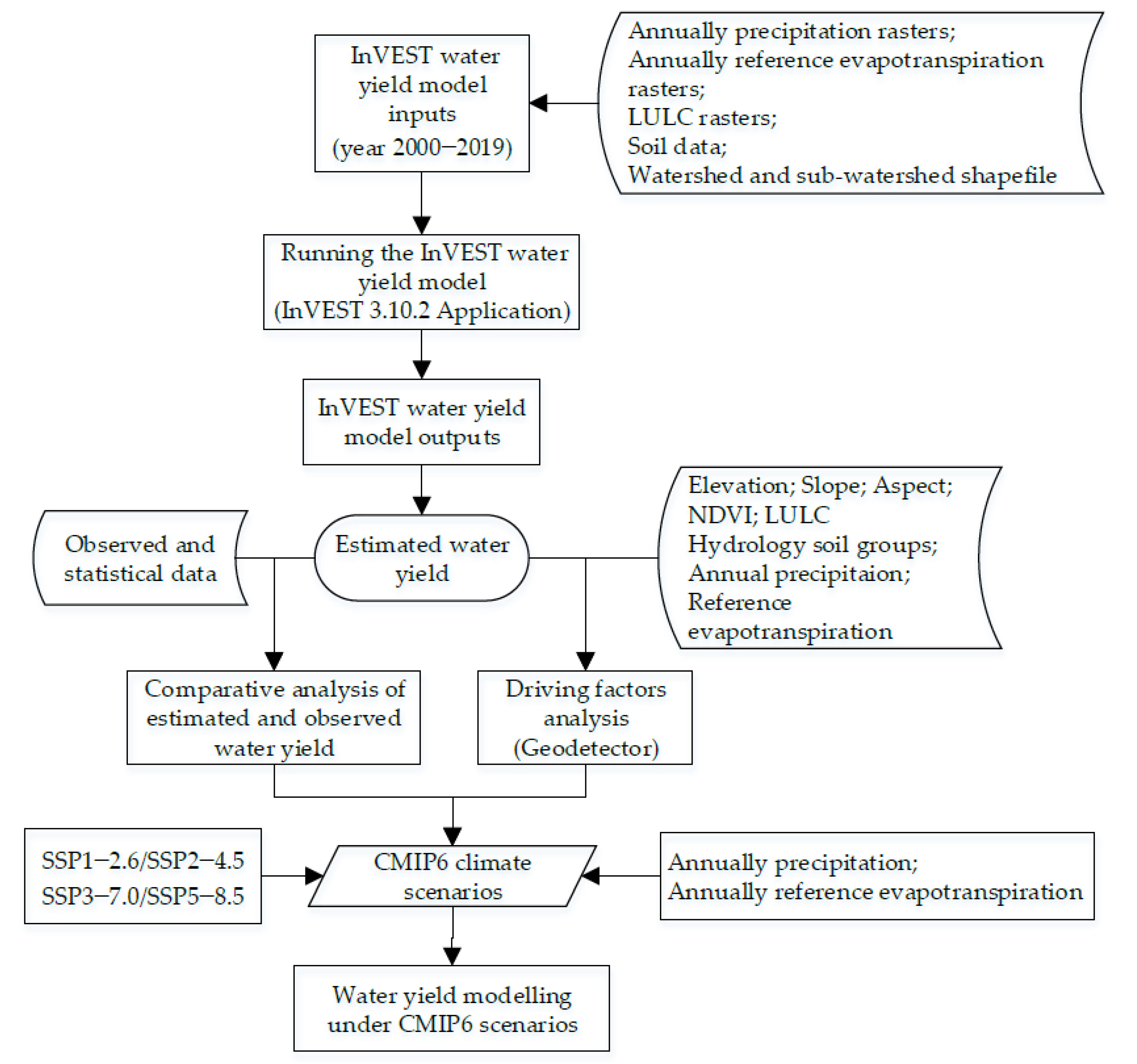
The research framework is shown in Figure 3. The main work of this article was as follows: (1) We simulated the spatial and temporal variations in water yield for the CLB over the past 20 years using open data and verified the reliability of the model in this study region using measured statistical data; (2) We elucidated the relationships between water yield and meteorological factors, topographic factors, soils, LULC, vegetation cover, and other factors in different hydrological years; (3) Based on the validated model, we predicted the spatial and temporal variations in water yield for the CLB under the CMIP6 climate change mode.

2.3.1. Water Yield Model

The water yield model in InVEST is designed to quantify the relative water yields of different basins or sub-basins. It calculates the annual water yield of a basin while taking into account the expected end use of the reservoir for hydropower production [48]. Although the contribution of hydropower generation in the CLB is relatively small [49], the total annual water production can provide many potential services, including agricultural irrigation, industrial water use, water supply, and hydropower generation. In this study, water production was simulated using the InVEST 3.10.2 software. The set of model equations is as follows.
Y X = ( 1 AET X P X _ ) · P X
AET X P X = 1 + PET X P X [ 1 + ( PET X P X ) ω ] 1 / ω
PET X = K C ( l X ) · ET OX
ω X = Z AWC X P X + 1 . 25
AWC X = Min ( rest . layer . depth , root . depth ) × PAWC
In the above formula, Y X represents the annual water production of each raster cell x; AET X represents the annual actual evapotranspiration; P X represents the annual precipitation; P E T X represents the reference evapotranspiration; ω X represents the non-physical parameters of natural climate-soil properties; ET OX represents the reference crop evapotranspiration of raster cell x; K C ( l X ) represents the plant (vegetation) evapotranspiration coefficient in a specific LULC type in the range [0,1.5]; ω X is an empirical parameter with 1.25 as a base; AWC X represents the effective soil water content (mm); Z is the empirical constant, also known as the seasonal constant; PAWC is the plant water content; rest . layer . depth is the maximum root depth of the soil and root; root . depth is the plant root depth.
The plant evapotranspiration coefficient (Kc) is strongly influenced by LULC. It is estimated by referring to the InVEST user guide [27] and the relevant literature from similar study regions [50], see Table 2. The Z parameter is continuously adjusted according to the results of the model calibration to make the relative error between the measured and modeled values as small as possible. The simulated water yield was found to be optimal when the Z parameter was 10.

2.3.2. Geodetector

The Geodetector software is designed to detect the driving forces of geographic phenomena by analyzing the spatial distribution characteristics of the phenomena [51]. The core purpose is to explore the strength of the relationship between the independent and dependent variables [52]. It consists of four main detectors: risk, factor, ecological, and interaction. In this paper, we used factor detectors and interaction detectors to identify the driving factors of water production and the interactions between these factors. The model is as follows.
q = 1 h = 1 L N h σ h 2 N σ 2 = 1 SSW SST
In the formula, h (1, ..., L) is the stratification of variable Y or factor X; N h and N are the number of cells in stratification h and the whole area, respectively; σ h 2 and σ 2 are the variance of Y values in stratification h and the whole area, respectively. SSW and SST are, respectively, the within sum of squares and the total sum of squares. q has the value range [0,1].
The driving analysis of water yield was analyzed using the open-source Geodetector software (http://www.geodetector.org/ (accessed on 30 June 2022)). Eight indicators were selected as independent variables, i.e., elevation, slope, aspect, NDVI, LULC, precipitation, reference evapotranspiration (RET), and hydrologic soil group (HSG). The independent variables were reclassified into six categories using the natural breakpoint method. By constructing a 2 km × 2 km fishing grid for the watershed, the information on independent and dependent variables at the center point of the fishing grid was extracted. The input datasets included 3470 rows.

3. Results and Discussion

3.1. Water Yield Simulation of CLB from 2000 to 2019

3.1.1. Interannual Variation

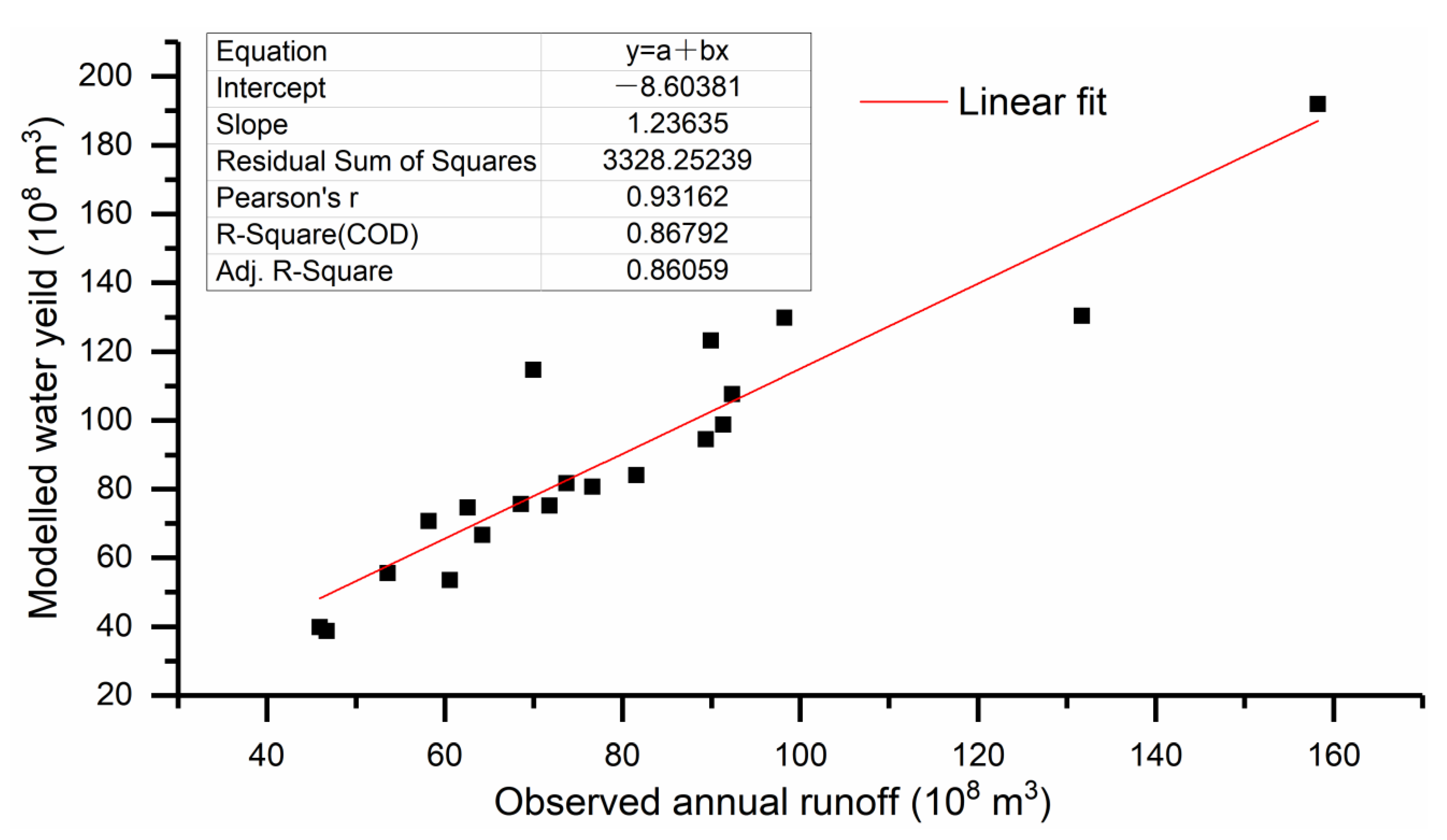
The water yield results simulated by the InVEST water yield model were compared with the measured statistical surface runoff data, and the best prediction model was obtained by continuously adjusting the parameters suited to the study region. The model calibration results are shown in Figure A1. There was a strong linear relationship between the annual water production simulated by the water yield model and the observed annual surface runoff from 2000 to 2019. The linear regression fitting equation was y = 1.2363x − 8.6038 (R2 = 0.868, p < 0.01), and the Pearson correlation coefficient was 0.93. This shows that the simulation of water production using the InVEST model is appropriate for the CLB.
The interannual variations in the simulated water yield and the observed statistical surface runoff data from 2000 to 2019 were shown in Figure 4. In terms of temporal changes, the model simulations showed consistent changes in the observed statistical runoff. The water yield from 2000 to 2019 in the CLB showed a fluctuating increasing trend, with three peaks in 2003, 2010, and 2016. The modeled water yields were, respectively, 130.43 × 10⁸ m3, 114.72 × 10⁸ m3, 191.98 × 10⁸ m3, and the observed runoffs were, respectively, 131.70 × 10⁸ m3, 69.93 × 10⁸ m3, and 158.25 × 10⁸ m3. The two lowest values were in 2001 and 2019; the modeled water yields were, respectively, 38.68 × 10⁸ m3 and 39.82 × 10⁸ m3, and the observed runoffs were, respectively, 46.72 × 10⁸ m3 and 45.94 × 10⁸ m3.
The model simulation results were overall slightly higher than the statistical data results, probably because the InVEST water yield model assumes that all water yields from each raster reach the basin outlet via subsurface runoff or surface runoff, while the observed statistical surface runoffs were monitored by hydrological stations and did not include a subsurface runoff component. Dong et al. used the SCS-CN model to estimate surface flow production in this study region, and they obtained the average values of surface runoff in the CLB from 2002 to 2006 as 1167.11 mm, 1363.57 mm, 946.05 mm, 1066.16 mm, and 1036.72 mm, respectively [53]. In this paper, the simulated annual water yield in the CLB showed relatively lower results, which respectively were 703.07 mm, 927.84 mm, 473.63 mm, 597.36 mm, and 530.50 mm from 2002 to 2006. However, the interannual trend was consistent with them as well as the annual precipitation change.

3.1.2. Spatial Variation

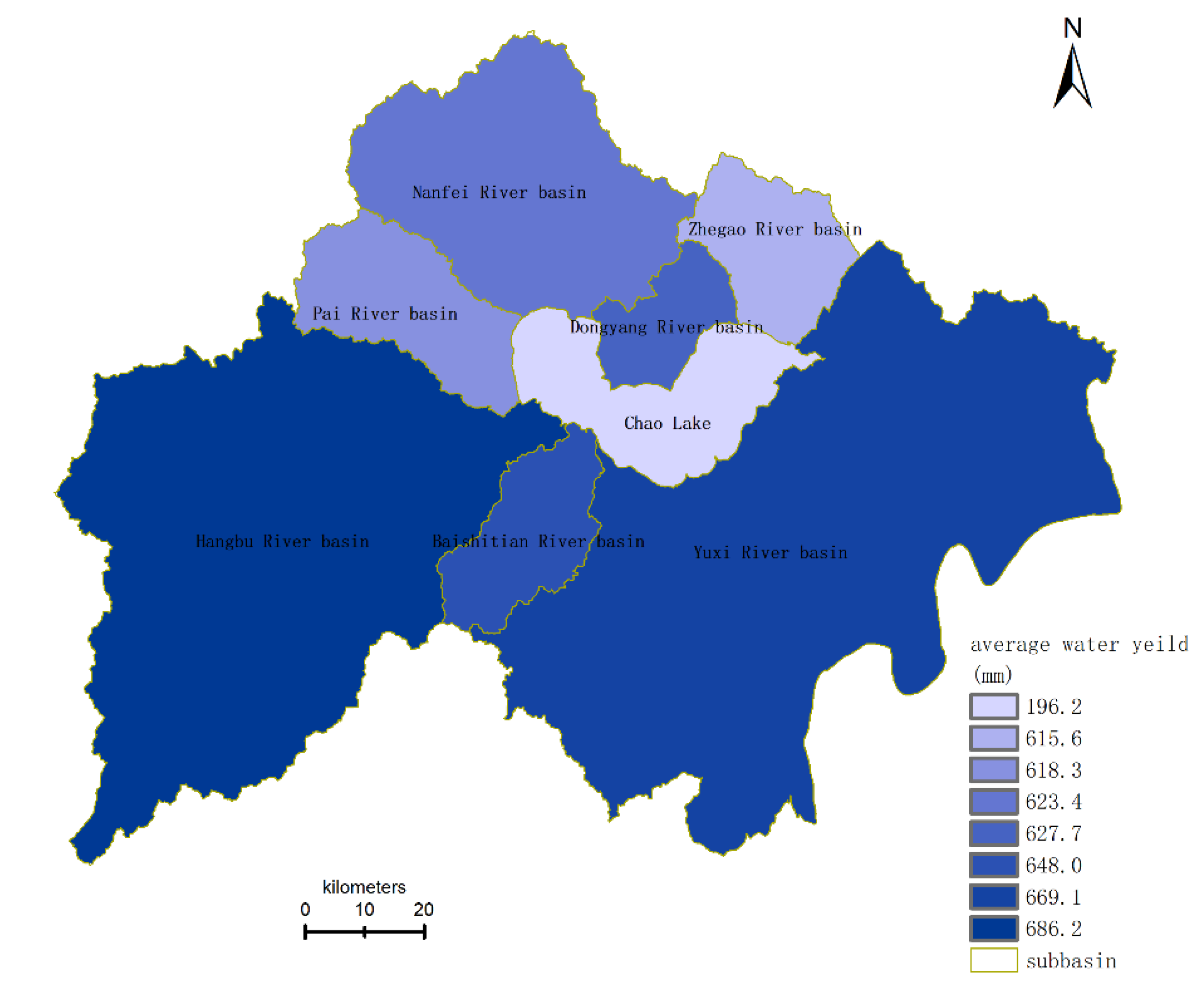
The annual average water yield of the sub-basin in the CLB from 2000 to 2019 is shown in Figure 5. The annual average water yield depth of the CLB was 633.8 ± 183.0 mm. The spatial distribution pattern indicated that the water yield was generally higher in the south than in the north. The Hangbu River Basin and the Yuxi River Basin contributed the highest amount of water yield at 686.2 mm and 669.1 mm, respectively. The differences in water yield in the sub-basins, except the Chaohu Lake water body, were not significant, probably because the use of regional and multi-year averages smoothed out the differences between annual and regional water yields. The spatial distribution of water yields from 2000 to 2019 was similar to the spatial distribution of annual mean precipitation, which was higher in the three southern sub-basins and lower in the northern sub-basins. The results of the qualitative analysis indicated that precipitation had a particularly strong effect on water yield.

3.2. Driving Factors Analysis

In this paper, we selected three typical years with the highest, lowest, and median water yields during the 20-year period, which were 2001, 2008, and 2016. We studied the driving factors of spatial variation in water yield in the CLB using Geodetector.

3.2.1. Univariate Analysis

Table 4 shows that the independent variables of the factors explained the spatial differentiation in the water yield of the CLB. By comparing the q-value and the p-value of each factor in the three years, the results show that the q-value of precipitation in 2016 was largest when the water yield was greatest. This explained 44% the spatial variation in the water yield of the CLB (p < 0.05). Secondly, the LULC and reference evapotranspiration, respectively, accounted for 36% and 17% (p < 0.05); the other factors accounted for little. The LULC explained 46% of the spatial variation in the water yield in 2001 (p < 0.05), followed by precipitation, with an explanatory percentage of 25%. The q-value of the LULC in 2008 was much higher than that of the other factors, followed by the vegetation index, which, respectively, accounted for 63% and 17% (p < 0.05).
The above analysis showed that, among the eight driving factors selected in this paper, LULC and precipitation had a greater impact on the water yield of the CLB, meaning they are the dominant natural factors affecting the water yield of the CLB, followed by the vegetation index and reference evapotranspiration. The topographic and soil factors had the least influence on water yield in the CLB.

3.2.2. Interaction Analysis

The interaction detector assessed whether every two independent variables acting together increased or decreased the explanatory percentage of the dependent variable. Table 5 shows that the interaction between the LULC and precipitation had the highest q-values: 0.71, 0.77, and 0.85. The explanatory percentage of the interaction between the two variables for water yield in 2001, 2008, and 2016 reached 71%, 77%, and 85%, respectively. The interaction between all factors enhanced the influence of the single factor on water yield in the CLB, showing a bi-enhancement and nonlinear enhancement relationship. The interaction between LULC and precipitation further increased its influence on water yield. The interaction detection results were consistent in different hydrological years. This indicates that the water yield spatial differentiation in the CLB was not caused by a single factor, but by the combined effect of different influencing factors.
The terrain of the CLB is high in the southwest and low in the northeast, generally inclined toward Chaohu Lake, with 75% of it being below 50 m in height. There are mountains in the southwest, hills and shallow mountains in the northeast, and plains in the southeast and along Chaohu Lake (Figure 1). The topographic factors, including elevation, slope, and aspect, accounted for little of the water production changes, mainly due to the flat terrain conditions. The forest ecosystem stands are relatively singular in the CLB. The soil and water conservation capacity is low. At present, more than 100 km2 of pure artificial poplar forest is aging. The capacity of carbon sink, soil, and water conservation has gradually weakened [54]. The NDVI and LULC factors, which are influenced by human activities, affected more spatial variations in the water yield. In the practice of river watershed resource management, we should consider different characteristics of the driving factors, as these driving factors interact to enhance the effects. We should implement scientific water resource allocation plans that match the regional natural conditions and effects of human activities to avoid unreasonable or strong man-made interference on land use, thus enhancing the pressure of regional water resource systems.

3.3. Spatial and Temporal Variations in Water Yield under Future Climate Change

3.3.1. Trend Analysis of Annual Precipitation and Annual Reference Evapotranspiration

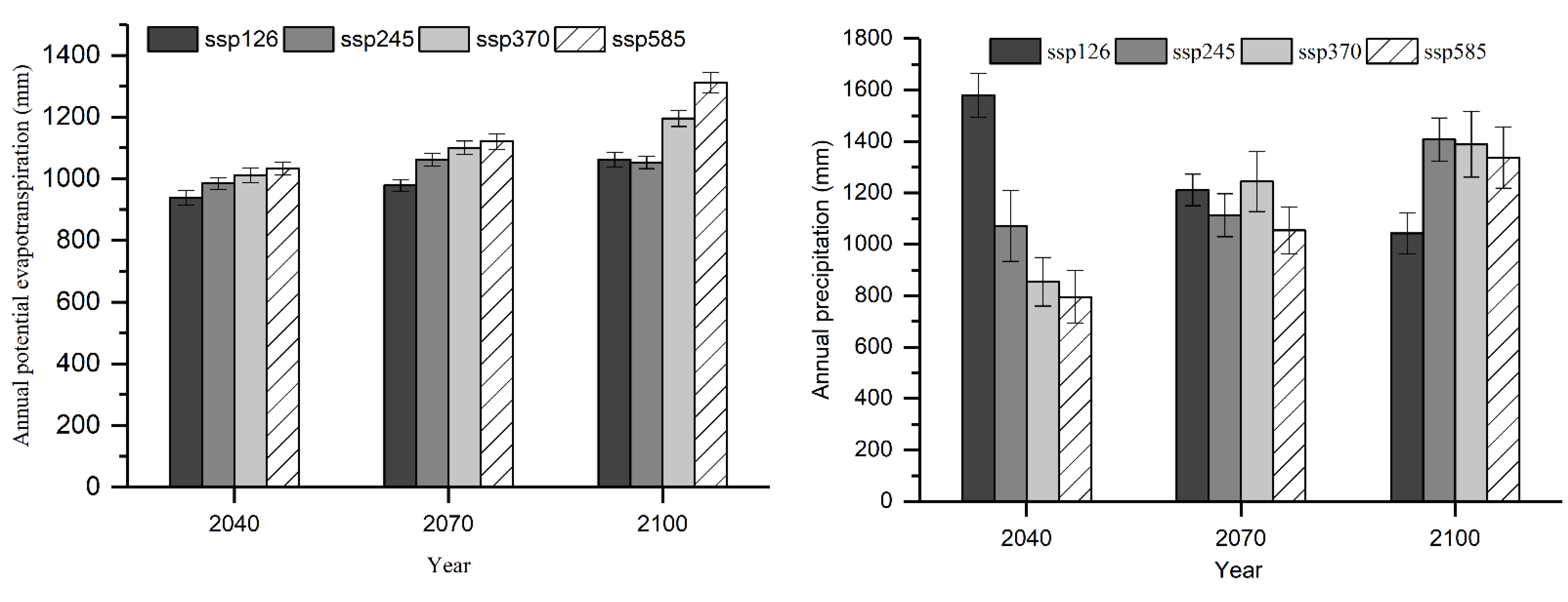
Figure 6 reflects the trends of annual precipitation and annual reference evapotranspiration for the four scenarios of SSP1-2.6, SSP2-4.5, SSP3-7.0, and SSP5-8.5 for three future years. The annual precipitation in this study region had a decreasing trend under the SSP1-2.6 scenario, with 23.2% and 34.0% decrease in precipitation in 2070 and 2100, respectively, compared with 2040. In contrast, the annual precipitation under three scenarios, SSP2-4.5, SSP3-7.0, and SSP5-8.5, had an increasing trend. Under the SSP2-4.5 scenario, the precipitation in 2070 and 2100 increased, respectively, by 3.8% and 31.3% compared with 2040. Under the SSP3-7.0 scenario, the precipitation in 2070 and 2100 increased, respectively, by 45.6% and 62.5%. Under the SSP8-8.5 scenario, the precipitation in 2070 and 2100 increased, respectively, by 32.5% and 68.1%.
The annual reference evapotranspiration in the study region under the four scenarios increased each year. It increased by 4.3% in 2070 and 13.2% in 2100 under SSP1-2.6; 7.9% in 2070 and 6.9% in 2100 under SSP2-4.5; 8.9% in 2070 and 18.3% in 2100 under SSP3-7.0; and 8.6% in 2070 and 27.0% in 2100 under SSP5-8.5. Annual reference evapotranspiration is correlated with temperature. The scenario with higher carbon emissions, which predicted higher atmospheric carbon dioxide (CO2) concentrations, included a higher estimation of annual reference evapotranspiration.
In addition to SSP1-2.6, the precipitation and evapotranspiration in the CLB increased under climate change scenarios, which was consistent with the results of Li [55] and Zhang [56] et al. regarding the Changbai Mountain Basin and the Upstream Basin of the Miyun Reservoir in China using the BCC-CSM2-MR model. Under global warming of 1.5 °C, 2 °C, and 3 °C, the average estimated total precipitation in China will increase by 5.3%, 8.6%, and 16.3% compared with current global warming. The total precipitation and heavy precipitation in the south of the Yangtze River Basin and near 40° N will increase to a notable degree [57].

3.3.2. Trend Analysis of Annual Water Yield

The annual precipitation and annual reference evapotranspiration data for the future scenarios were substituted into the InVEST model to obtain the water yield of the CLB for the four scenarios for the three future years. The mean values for each sub-basin were calculated, as shown in Figure 7. Under the SSP1-2.6 scenario, the annual water yield decreased with decreasing annual precipitation for the three years, and the total annual water yield in 2070 seemed to be roughly equivalent to the average results from 2000 to 2019. The differences in water yield in 2070 and 2100 compared to 2040 for each sub-basin were not significant, except for Chaohu Lake. The reductions ranged from 35.8% to 39.5% in 2070 and 57.6% to 62% in 2100, compared to 2040.
Under the SSP2-4.5 scenario, the annual water yield increased with the increase in annual precipitation in the three years, especially in the Pai River Basin and Nanfei River Basin in the northern CLB, which are located in the megalopolis of Hefei, with an average increase of 5.6% and 71.0% in 2070 and 2100 compared to 2040. In the south, the Baishitian River Basin and the Yuxi River Basin had the smallest increase in water production. The Hangbu River Basin and the Yuxi River Basin had higher water production due to their larger areas, with predicted values of 32.4 × 10⁸ m3 and 40.3 × 10⁸ m3 in 2100 under the SSP2-4.5 scenario, respectively.
Under the SSP3-7.0 and SSP5-8.5 scenarios, the average increase reached 108.5% and 139.8% in 2070 and 85.9% and 159.5% in 2100 compared with 2040, with annual water production increasing with annual precipitation in all three years. The spatial differences in the increases over the sub-basins were consistent with the pattern of SSP2-4.5, with greater increases in the northern sub-basins than in the southern sub-basins. SSP3-7.0, which represents the moderate baseline results produced by the energy systems model, was used in conjunction with SSP5-8.5 (worst-case scenario) to simulate global warming trends without climate policy intervention. The increase in water yield was significantly higher than SSP2-4.5, in which social vulnerability and radiative forcing are moderate.
In addition, a longitudinal comparison in Figure 7 reflected the impact of different carbon emission scenarios on water production. Under the four scenarios of SSP1-2.6, SSP2-4.5, SSP3-7.0, and SSP5-8.5, the total water production in the CLB in 2040 would be 134.8 × 10⁸ m3, 63.5 × 10⁸ m3, 37.2 × 10⁸ m3, and 30.2 × 10⁸ m3; in 2070, the total water production would be 80.8 × 10⁸ m3, 63.0 × 10⁸ m3, 76.4 × 10⁸ m3, and 52.7 × 10⁸ m3; in 2100, the total water production would be 54.8 × 10⁸ m3, 100.9 × 10⁸ m3, 87.6 × 10⁸ m3, and 73.8 × 10⁸ m3. With an increase in carbon emission intensity, the overall trend of water production decreased, and the spatial divergence was greater in the northern sub-basin than in the southern sub-basin.
The CLB is affected by an intergrade subtropical monsoon climate situated between subtropical and warm temperate zones. The spatial and temporal distribution of rainfall in the region is uneven, and it is concentrated in summer. There is much intense rainfall, often resulting in flood disasters. Chaohu Lake has a wide water surface and slow flow rate, which are the characteristics of a typical plain lake at the lower reaches of the Yangtze River. It has a growing water supply and takes in drainage from large provincial cities. At the same time, due to the extension of the water exchange cycle caused by the construction of a sluice at the mouth of the lake in 1962, the water purification capacity of the lake was reduced. There is great pressure on the quality and quantity of the water resources of the CLB, especially in the northern watershed, due to a high degree of urbanization and sharp conflicts between population and land.

3.4. Limitations

The three main inputs of the InVEST water yield model are LULC, climatic factors, and soil parameters, which can influence the water yield by changing the hydrological cycle. The results of this paper showed that climatic factors had a strong influence on water production in the CLB. Therefore, we assumed that inputs other than precipitation and reference evapotranspiration would remain constant in all future scenarios, and we quantified the impact of future climate change on water yield in the CLB. The prediction of future land use changes in the CLB is subject to uncertainty, as land use changes in the CLB are mainly derived from government investment and sector-driven policy demands rather than a natural demand for land from socioeconomic development [58]. The shortcoming of this study was that we could not accurately simulate water changes with high-frequency variability characteristics using the InVEST model, so the interaction between future LULC changes and climate change was not considered. In addition, the results showed an opposite trend between SSP1-2.6 and other SSPs, which were decided by the input precipitation that was derived from the climate model. The use of a single climate model in this study increased the uncertainty of the simulation results in driving the hydrological model, and an ensemble-based multi-climate model should be used to improve the simulation accuracy and spatial resolution by overcoming the limitation of relying on a single data source.

4. Conclusions

In this study, we evaluated the applicability of the InVEST water yield model in a typical lake basin in the middle and lower reaches of the Yangtze River in China. Then, we quantified the driving factors of water yield and their interactions using a new spatial statistical method (Geodetector). Furthermore, we analyzed the effects of future climate changes in precipitation and temperature on water yield in the CLB by applying CMIP6 climate model data to the InVEST model:
(1)
The results showed that the water yield simulated using the InVEST model had good applicability in this study region. There was a strong linear relationship between the simulated water yield and the measured surface runoff (y = 1.2363x − 8.6038, R2 = 0.868, p < 0.01), and the Pearson correlation coefficient was 0.93. The annual average water yield depth in the CLB from 2000 to 2019 was 633.8 ± 183.0 mm, which was generally higher in the south than in the north;
(2)
The results of the Geodetector analysis showed that the explanatory percentage of interaction between the precipitation and LULC for water yield in 2001, 2008, and 2016 reached 71%, 77%, and 85%, respectively, and these were the two dominant factors affecting water yield in the CLB;
(3)
The results of water yield simulations based on downscale-corrected BCC-CSM2-MR model data showed that the average annual water yield in the CLB increased with increasing precipitation under the SSP2-4.5, SSP3-7.0, and SSP5-8.5 scenarios, and it declined under the SSP1-2.6 scenario. The average annual water yield increased by 5.6%, 108.5%, and 85.9% in 2070 compared with 2040 under the SSP2-4.5, SSP3-7.0, and SSP5-8.5 scenarios, and it increased by 71%, 139.8%, and 159.5% in 2100 compared with 2040 under the SSP2-4.5, SSP3-7.0, and SSP5-8.5 scenarios. The overall trend of the water yield decreased with increases in carbon emission intensity.
The results of this study will help to understand the potential impact of future climate change on the water supply in the region. The general increase trend of watershed water yield will probably cause more flood and urban water logging, the decline of wetland vegetation, and geological disaster. Managers should pay attention to these issues and develop a comprehensive plan accordingly.
The water yield model of InVEST based on a simplified hydrological process was further proved accurate on an annual scale in our study, which can be generalized to other regions for evaluating water resources under multi scenarios, such as climate change and intensive land development. It is useful for researchers and managers who are short of sufficient expertise and time. The framework and methods used in the study can be able to apply in the further prediction of annual water production changes in the short or medium term, in response to LULC and climate change.

Author Contributions

Conceptualization, T.Z. and H.X.; methodology, T.Z. and Q.G.; validation, T.Z., Q.G. and Q.W.; formal analysis, T.Z. and Q.G.; investigation, H.X.; resources, T.Z. and Q.W.; data curation, T.Z., C.Z. and Z.C.; writing—original draft preparation, T.Z., Q.G. and H.X.; writing—review and editing, T.Z., H.X. and Q.W.; visualization, Y.Y. and H.H.; supervision, H.X.; project administration, T.Z.; funding acquisition, T.Z. All authors have read and agreed to the published version of the manuscript.

Funding

This research was supported by the Natural Science Research Project of University in Anhui Province, grant number KJ2019A0763 and KJ2020JD07; the Natural Science Foundation of Anhui Province, grant number 2108085QD151; the Science and Technology Program of Hubei Provincial Education Department, grant number Q20182803, the Research Fund of Anhui Jianzhu University, grant number 2018QD27.

Institutional Review Board Statement

Not applicable.

Informed Consent Statement

Not applicable.

Data Availability Statement

The meteorological data from 2000 to 2019 were obtained from the daily dataset of Chinese terrestrial climate information (V3.0), National Meteorological Science Data Center (NMSDC) (http://data.cma.cn/ (accessed on 8 April 2021)); the LULC rasters and NDVI were obtained from the Resource and Environment Science and Data Center (https://www.resdc.cn/ (accessed on 26 March 2021)); the soil map was obtained from the Harmonized World Soil Database (v1.2) (https://www.fao.org/soils-portal/soil-survey/soil-maps-and-databases/harmonized-world-soil-database-v12/en/ (accessed on 6 May 2021)); the observed annual surface runoff was obtained from the Anhui Statistical Yearbook on the Anhui Provincial Bureau of Statistics website (http://tjj.ah.gov.cn/ (accessed on 30 June 2022)); the DEM, watersheds and sub-watersheds boundaries were obtained from the Lake-Watershed Science SubCenter, National Earth System Science Data Center, National Science & Technology Infrastructure of China (http://gre.geodata.cn (accessed on 29 June 2021)); the CMIP6 data were obtained from the World Climate Research Programme (WCRP, https://esgf-data.dkrz.de/search/cmip6-dkrz/ (accessed on 25 July 2022)).

Conflicts of Interest

The authors declare no conflict of interest.

Appendix A

Figure A1. Scatter plot fitting of simulated water yield and measured runoff.
Sustainability 14 14080 g0a1

References

  1. Liu, S.; Yin, Y.; Liu, X.; Cheng, F.; Yang, J.; Li, J.; Dong, S.; Zhu, A. Ecosystem Services and Landscape Change Associated with Plantation Expansion in a Tropical Rainforest Region of Southwest China. Ecol. Model. 2017, 353, 129–138. [Google Scholar] [CrossRef]
  2. Ping, L.; Zheng, X.; Chen, J.; Zhang, Q.; Li, J.; Bo, W. Characteristic Analysis of Ecosystem Service Value of Water System in Taiyuan Urban District Based on LUCC. Int. J. Agric. Biol. Eng. 2016, 9, 153–165. [Google Scholar]
  3. Fu, B.J.; Zhou, G.Y.; Bai, Y.F.; Song, C.C.; Xie, G.D. The Main Terrestrial Ecosystem Services and Ecological Security in China. Adv. Earth Sci. 2009, 24, 571–576. [Google Scholar]
  4. van Vliet, M.T.H.; Jones, E.R.; Flörke, M.; Franssen, W.H.P.; Hanasaki, N.; Wada, Y.; Yearsley, J.R. Global Water Scarcity Including Surface Water Quality and Expansions of Clean Water Technologies. Environ. Res. Lett. 2021, 16, 024020. [Google Scholar] [CrossRef]
  5. MA (Millennium Ecosystem Assessment). Ecosystem and Human Well-Being; Island Press: Washington, DC, USA, 2005. [Google Scholar]
  6. Le Maitre, D.C.; Milton, S.J.; Jarmain, C.; Colvin, C.A.; Saayman, I.; Vlok, J.H. Linking Ecosystem Services and Water Resources: Landscape-Scale Hydrology of the Little Karoo. Front. Ecol. Environ. 2007, 5, 261–270. [Google Scholar] [CrossRef]
  7. Tao, F.; Zhang, Z. Dynamic Responses of Terrestrial Ecosystems Structure and Function to Climate Change in China. J. Geophys. Res. 2010, 115, G03003. [Google Scholar] [CrossRef]
  8. Nedkov, S.; Campagne, S.; Borisova, B.; Krpec, P.; Prodanova, H.; Kokkoris, I.P.; Hristova, D.; Le Clec’h, S.; Santos-Martin, F.; Burkhard, B.; et al. Modeling Water Regulation Ecosystem Services: A Review in the Context of Ecosystem Accounting. Ecosyst. Serv. 2022, 56, 101458. [Google Scholar] [CrossRef]
  9. Boumans, R.; Costanza, R.; Farley, J.; Wilson, M.A.; Portela, R.; Rotmans, J.; Villa, F.; Grasso, M. Modeling the Dynamics of the Integrated Earth System and the Value of Global Ecosystem Services Using the GUMBO Model. Ecol. Econ. 2002, 41, 529–560. [Google Scholar] [CrossRef]
  10. Schägner, J.P.; Brander, L.; Maes, J.; Hartje, V. Mapping Ecosystem Services’ Values: Current Practice and Future Prospects. Ecosyst. Serv. 2013, 4, 33–46. [Google Scholar] [CrossRef] [Green Version]
  11. Benra, F.; De Frutos, A.; Gaglio, M.; Alvarez-Garreton, C.; Felipe-Lucia, M.; Bonn, A. Mapping Water Ecosystem Services: Evaluating InVEST Model Predictions in Data Scarce Regions. Environ. Model. Softw. 2021, 138, 104982. [Google Scholar] [CrossRef]
  12. Arnold, J.G.; Moriasi, D.N.; Gassman, P.W.; Abbaspour, K.C.; White, M.J.; Srinivasan, R.; Santhi, C.; Harmel, R.D.; van Griensven, A.; van Liew, M.W.; et al. SWAT: Model Use, Calibration, and Validation. Trans. ASABE 2012, 55, 1491–1508. [Google Scholar] [CrossRef]
  13. Abbaspour, K.C.; Rouholahnejad, E.; Vaghefi, S.; Srinivasan, R.; Yang, H.; Kløve, B. A Continental-Scale Hydrology and Water Quality Model for Europe: Calibration and Uncertainty of a High-Resolution Large-Scale SWAT Model. J. Hydrol. 2015, 524, 733–752. [Google Scholar] [CrossRef]
  14. Ma, L.; He, C.; Bian, H.; Sheng, L. MIKE SHE Modeling of Ecohydrological Processes: Merits, Applications, and Challenges. Ecol. Eng. 2016, 96, 137–149. [Google Scholar] [CrossRef]
  15. Torres, M.A.; Nikolskii, I.; Martínez Miranda, M.E.; Martínez, M.R. Evaluación Hidrológica de La Cuenca Del Río Teapa, Utilizando El Modelo MIKE-SHE. Tecnol. Y Cienc. Del Agua 2018, 9, 130–146. [Google Scholar] [CrossRef]
  16. Singh, P.K.; Gaur, M.L.; Mishra, S.K.; Rawat, S.S. An Updated Hydrological Review on Recent Advancements in Soil Conservation Service-Curve Number Technique. J. Water Clim. Chang. 2010, 1, 118–134. [Google Scholar] [CrossRef]
  17. Verma, R.K.; Verma, S.; Mishra, S.K.; Pandey, A. SCS-CN-Based Improved Models for Direct Surface Runoff Estimation from Large Rainfall Events. Water Resour. Manag. 2021, 35, 2149–2175. [Google Scholar] [CrossRef]
  18. He, F.; Jin, J.; Zhang, H.; Yuan, L. The Change of Ecological Service Value and the Promotion Mode of Ecological Function in Mountain Development Using InVEST Model. Arab. J. Geosci. 2021, 14, 510. [Google Scholar] [CrossRef]
  19. Zhang, H.; Feng, J.; Zhang, Z.; Liu, K. Regional spatial management based on supply-demand risk of ecosystem services—A case study of the Fenghe River watershed. Int. J. Environ. Res. Public Health 2020, 17, 4112. [Google Scholar] [CrossRef]
  20. Dennedy-Frank, P.J.; Muenich, R.L.; Chaubey, I.; Ziv, G. Comparing Two Tools for Ecosystem Service Assessments Regarding Water Resources Decisions. J. Environ. Manag. 2016, 177, 331–340. [Google Scholar] [CrossRef] [Green Version]
  21. Butsic, V.; Shapero, M.; Moanga, D.; Larson, S. Using InVEST to Assess Ecosystem Services on Conserved Properties in Sonoma County, CA. Calif. Agric. 2017, 71, 81–89. [Google Scholar] [CrossRef] [Green Version]
  22. Kim, S.; Jung, Y. Application of the InVEST Model to Quantify the Water Yield of North Korean Forests. Forests 2020, 11, 804. [Google Scholar] [CrossRef]
  23. Nematollahi, S.; Fakheran, S.; Kienast, F.; Jafari, A. Application of InVEST Habitat Quality Module in Spatially Vulnerability Assessment of Natural Habitats (Case Study: Chaharmahal and Bakhtiari Province, Iran). Environ. Monit. Assess. 2020, 192, 487. [Google Scholar] [CrossRef] [PubMed]
  24. Hamel, P.; Chaplin-Kramer, R.; Sim, S.; Mueller, C. A New Approach to Modeling the Sediment Retention Service (InVEST 3.0): Case Study of the Cape Fear Catchment, North Carolina, USA. Sci. Total Environ. 2015, 524, 166–177. [Google Scholar] [CrossRef]
  25. Caro, C.; Marques, J.C.; Cunha, P.P.; Teixeira, Z. Ecosystem Services as a Resilience Descriptor in Habitat Risk Assessment Using the InVEST Model. Ecol. Indic. 2020, 115, 106426. [Google Scholar] [CrossRef]
  26. Scordo, F.; Lavender, T.; Seitz, C.; Perillo, V.; Rusak, J.; Piccolo, M.; Perillo, G. Modeling Water Yield: Assessing the Role of Site and Region-Specific Attributes in Determining Model Performance of the InVEST Seasonal Water Yield Model. Water 2018, 10, 1496. [Google Scholar] [CrossRef] [Green Version]
  27. Sharp, R.; Douglass, J.; Wolny, S.; Arkema, K.; Bernhardt, J.; Bierbower, W.; Chaumont, N.; Denu, D.; Fisher, D.; Glowinski, K.; et al. InVEST 3.11.0.post56+ug.gfa89dd9 User’s Guide. The Natural Capital Project, Stanford University, University of Minnesota, The Nature Conservancy, and World Wildlife Fund. 2020. Available online: https://naturalcapitalproject.stanford.edu/software/invest (accessed on 15 January 2022).
  28. Peng, L.-C.; Lin, Y.-P.; Chen, G.-W.; Lien, W.-Y. Climate Change Impact on Spatiotemporal Hotspots of Hydrologic Ecosystem Services: A Case Study of Chinan Catchment, Taiwan. Water 2019, 11, 867. [Google Scholar] [CrossRef] [Green Version]
  29. Liu, R.; Niu, X.; Wang, B.; Song, Q. InVEST Model-Based Spatiotemporal Analysis of Water Supply Services in the Zhangcheng District. Forests 2021, 12, 1082. [Google Scholar] [CrossRef]
  30. Yang, D.; Liu, W.; Tang, L.; Chen, L.; Li, X.; Xu, X. Estimation of Water Provision Service for Monsoon Catchments of South China: Applicability of the InVEST Model. Landsc. Urban Plan. 2019, 182, 133–143. [Google Scholar] [CrossRef]
  31. Redhead, J.W.; Stratford, C.; Sharps, K.; Jones, L.; Ziv, G.; Clarke, D.; Oliver, T.H.; Bullock, J.M. Empirical Validation of the InVEST Water Yield Ecosystem Service Model at a National Scale. Sci. Total Environ. 2016, 569–570, 1418–1426. [Google Scholar] [CrossRef] [Green Version]
  32. Yang, X.; Chen, R.; Meadows, M.E.; Ji, G.; Xu, J. Modelling Water Yield with the InVEST Model in a Data Scarce Region of Northwest China. Water Supply 2020, 20, 1035–1045. [Google Scholar] [CrossRef]
  33. Cong, W.; Sun, X.; Guo, H.; Shan, R. Comparison of the SWAT and InVEST Models to Determine Hydrological Ecosystem Service Spatial Patterns, Priorities and Trade-Offs in a Complex Basin. Ecol. Indic. 2020, 112, 106089. [Google Scholar] [CrossRef]
  34. Yang, D.; Liu, W.; Xu, C.; Tao, L.; Xu, X. Integrating the InVEST and SDSM Model for Estimating Water Provision Services in Response to Future Climate Change in Monsoon Basins of South China. Water 2020, 12, 3199. [Google Scholar] [CrossRef]
  35. Yan, Y.; Guan, Q.; Wang, M.; Su, X.; Wu, G.; Chiang, P.; Cao, W. Assessment of Nitrogen Reduction by Constructed Wetland Based on InVEST: A Case Study of the Jiulong River Watershed, China. Mar. Pollut. Bull. 2018, 133, 349–356. [Google Scholar] [CrossRef]
  36. Zhu, H.; Jiang, Z.; Li, J.; Li, W.; Sun, C.; Li, L. Does CMIP6 Inspire More Confidence in Simulating Climate Extremes over China? Adv. Atmos. Sci. 2020, 37, 1119–1132. [Google Scholar] [CrossRef]
  37. Li, J.; Chen, X.; Kurban, A.; Van de Voorde, T.; De Maeyer, P.; Zhang, C. Coupled SSPs-RCPs Scenarios to Project the Future Dynamic Variations of Water-Soil-Carbon-Biodiversity Services in Central Asia. Ecol. Indic. 2021, 129, 107936. [Google Scholar] [CrossRef]
  38. Zhou, T.; Zou, L.; Chen, X. Commentary on the Coupled Model Intercomparison Project Phase 6 (CMIP6). Clim. Change Res. 2019, 15, 445–456. [Google Scholar]
  39. Yazdandoost, F.; Moradian, S.; Izadi, A.; Aghakouchak, A. Evaluation of CMIP6 Precipitation Simulations across Different Climatic Zones: Uncertainty and Model Intercomparison. Atmos. Res. 2021, 250, 105369. [Google Scholar] [CrossRef]
  40. Guo, B.; Jin, X.; Fang, Y.; Zhou, Y. Evaluation of Sustainable Regional Development Combining Remote Sensing Data and Ecological Constraints: A Case Study of Chaohu Basin, China. Sustainability 2020, 12, 9836. [Google Scholar] [CrossRef]
  41. Wen, M.; Zhang, T.; Li, L.; Chen, L.; Hu, S.; Wang, J.; Liu, W.; Zhang, Y.; Yuan, L. Assessment of Land Ecological Security and Analysis of Influencing Factors in Chaohu Lake Basin, China from 1998–2018. Sustainability 2021, 13, 358. [Google Scholar] [CrossRef]
  42. Widmoser, P. A Discussion on and Alternative to the Penman-Monteith Equation. Agric. Water Manag. 2009, 96, 711–721. [Google Scholar] [CrossRef]
  43. Zhou, W.; Liu, G.; Pan, J.; Feng, X. Distribution of Available Soil Water Capacity in China. J. Geogr. Sci. 2005, 15, 3–12. [Google Scholar] [CrossRef]
  44. Feng, J.; Wei, W.; Feng, Q. The Runoff Curve Number of SCS-CN Method in Loess Hilly Region. Acta Ecol. Sin. 2021, 41, 4170–4181. [Google Scholar]
  45. Arnold, J.G.; Kiniry, J.R.; Srinivasan, R.; Williams, J.R.; Haney, E.B. Soil and Water Assessment Tool Input/Output File Documentation. Version 2009. 2011. Available online: https://swat.tamu.edu/docs/ (accessed on 15 December 2021).
  46. Hamadalnel, M.; Zhu, Z.; Gaber, A.; Iyakaremye, V.; Ayugi, B. Possible Changes in Sudan’s Future Precipitation under the High and Medium Emission Scenarios Based on Bias Adjusted GCMs. Atmos. Res. 2022, 269, 106036. [Google Scholar] [CrossRef]
  47. Xu, C.-Y.; Singh, V.P. Evaluation and Generalization of Temperature-Based Methods for Calculating Evaporation. Hydrol. Process. 2001, 15, 305–319. [Google Scholar] [CrossRef]
  48. Fu, B.; Wang, Y.K.; Xu, P.; Yan, K.; Li, M. Value of Ecosystem Hydropower Service and Its Impact on the Payment for Ecosystem Services. Sci. Total Environ. 2014, 472, 338–346. [Google Scholar] [CrossRef]
  49. Zhang, Z.; Gao, J.; Gao, Y. The Influences of Land Use Changes on the Value of Ecosystem Services in Chaohu Lake Basin, China. Environ. Earth Sci. 2015, 74, 385–395. [Google Scholar] [CrossRef]
  50. Ma, L.; Sun, R.; Kazemi, E.; Pang, D.; Zhang, Y.; Sun, Q.; Zhou, J.; Zhang, K. Evaluation of Ecosystem Services in the Dongting Lake Wetland. Water 2019, 11, 2564. [Google Scholar] [CrossRef] [Green Version]
  51. Wang, J.; Xu, C. Geodetector: Principle and Prospective. Acta Geogr. Sin. 2017, 72, 116–134. [Google Scholar]
  52. Su, Y.; Li, T.; Cheng, S.; Wang, X. Spatial Distribution Exploration and Driving Factor Identification for Soil Salinisation Based on Geodetector Models in Coastal Area. Ecol. Eng. 2020, 156, 105961. [Google Scholar] [CrossRef]
  53. Dong, W.; Cheng, X.; Zhang, Q.; Zhao, Y.; Han, P. Application of SCS-CN Model Estimating Surface Runoff to Chaohu Lake Basin. Bull. Soil Water Conserv. 2012, 32, 174–177+187. [Google Scholar] [CrossRef]
  54. Xie, S.; Zhu, H.; Tang, X.; Guo, J. Ecological Protection and Restoration of Mountain-river-forest-farmland-lake-grassland System in Chaohu Lake Basin. Available online: https://kns.cnki.net/kcms/detail/32.1356.TV.20220610.1347.002.html (accessed on 10 July 2022).
  55. Li, Z.; Cao, Y.; Duan, Y.; Jiang, Z.; Sun, F. Simulation and Prediction of the Impact of Climate Change Scenarios on Runoff of Typical Watersheds in Changbai Mountains, China. Water 2022, 14, 792. [Google Scholar] [CrossRef]
  56. Zhang, J.; Ma, S.; Song, Y. Hydrological and Water Quality Simulation and Future Runoff Prediction under CMIP6 Scenario in the Upstream Basin of Miyun Reservoir. J. Water Clim. Chang. 2022, 13, 2505–2530. [Google Scholar] [CrossRef]
  57. Zhu, H.; Jiang, Z.; Li, L. Projection of Climate Extremes in China, an Incremental Exercise from CMIP5 to CMIP6. Sci. Bull. 2021, 66, 2528–2537. [Google Scholar] [CrossRef]
  58. Fan, S.; Liu, Y.; Cheng, C.; Zhang, H.; Yu, R.; Lv, J. Land Use Change and Driving Mechanism in Rapid Urbanization Region-A Case Study at Chaohu River Basin. Bull. Soil Water Conserv. 2017, 37, 253–260. [Google Scholar] [CrossRef]
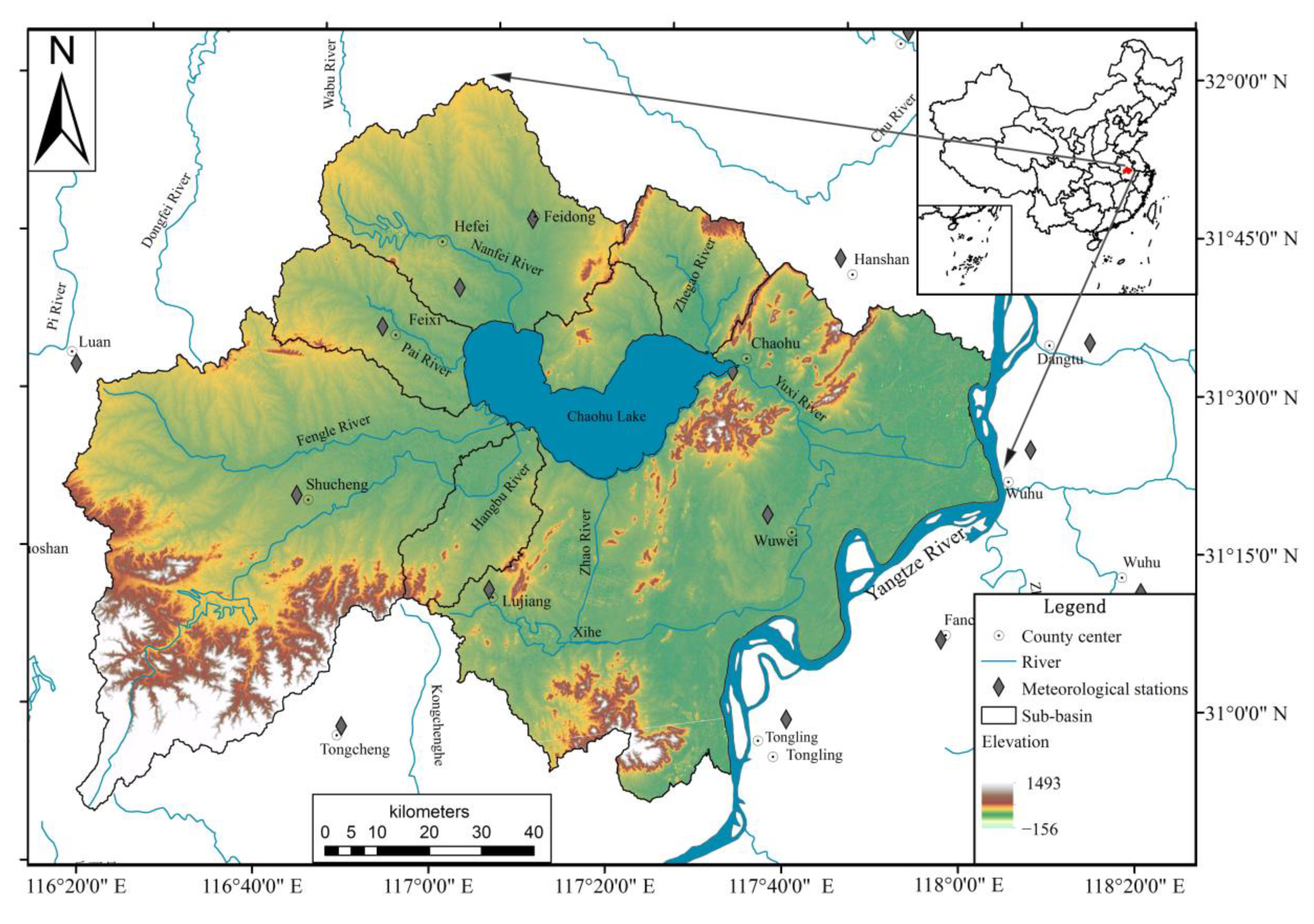
Figure 1. The location of the CLB.
Sustainability 14 14080 g001
Figure 2. Statistical downscaling results of monthly average temperature and monthly precipitation.
Sustainability 14 14080 g002
Figure 3. Technology roadmap for research work.
Sustainability 14 14080 g003
Figure 4. Comparison results between simulated water production and measured runoff, 2000–2019.
Sustainability 14 14080 g004
Figure 5. Multi-year average spatial distribution of water production in the CLB from 2000 to 2019.
Sustainability 14 14080 g005
Figure 6. Changes in annual precipitation and annual reference evapotranspiration under SSP scenarios.
Sustainability 14 14080 g006
Figure 7. Spatial distribution of annual water production in the CLB under four SSP scenarios.
Sustainability 14 14080 g007
Table 1. Sources of datasets for model running.
Data ItemsData Sources
Annual precipitation rasters from 2000 to 2019Daily dataset of Chinese terrestrial climate information (V3.0), National Meteorological Science Data Center (NMSDC) (http://data.cma.cn/ (accessed on 8 April 2021))
Annual reference evapotranspiration rasters from 2000 to 2019Daily dataset of Chinese terrestrial climate information (V3.0), National Meteorological Science Data Center (NMSDC) (http://data.cma.cn/ (accessed on 8 April 2021))
Land use and land cover rasters of 2000, 2005, 2010, 2015, 2018Resource and Environment Science and Data Center (http://www.resdc.cn/ (accessed on 26 March 2021))
Plant available water contentSoil map based Harmonized World Soil Database (v1.2) (https://www.fao.org/soils-portal/soil-survey/soil-maps-and-databases/harmonized-world-soil-database-v12/en/ (accessed on 6 May 2021))
Root restricting layer depth (Raster)Soil map based Harmonized World Soil Database (v1.2) (https://www.fao.org/soils-portal/soil-survey/soil-maps-and-databases/harmonized-world-soil-database-v12/en/ (accessed on 6 May 2021))
Watersheds and sub-watersheds Lake-Watershed Science SubCenter, National Earth System Science Data Center, National Science & Technology Infrastructure of China (http://gre.geodata.cn (accessed on 29 June 2021))
Table 2. Classification of LULC and evapotranspiration coefficient (Kc).
LULC Level 1 TypeLULC Level 2 TypeKc
CodeNameCodeName
1Cultivated land11Paddy field0.65
12Dry land0.65
2Woodland21Forested land1
22Bushlands0.398
23Sparse woodlands1
24Other woodlands1
3Grassland31High coverage grass0.65
32Medium coverage grass0.65
33Low coverage grass0.65
4Waters41Canals1.2
42Lakes1.2
43Reservoir pits1.2
46Beach1.2
5Urban and rural areas, industrial and mining, residential land51Town land0.3
52Rural residential area0.3
53Other construction land0.3
6Unused land65Bare land0.5
66Bare rock gravel0.5
Table 3. Hydrological soil group division criteria.
Hydrological Soil GroupABCD
Minimum infiltration rate>7.263.81–7.261.27–3.810.00–1.27
Saturated hydraulic conductivity (Ks, mm/h)>18018–1801.8–18<1.8
Soil textureSandy, loamy, sandy loamLoam, silt loamSandy clay loamClay loam, silt clay, sand clay, silt clay, clay
Table 4. q-value and p-value of Geodetector factor detection.
StatisticsYearElevationSlopeAspectHSGAETPrecipitationRETNDVILULC
q-value20010.04 0.020.060.050.250.160.130.460.04
20080.02 0.010.100.120.100.050.170.630.02
20160.03 0.020.070.080.440.170.110.360.03
p-value20010.000.000.000.000.000.000.000.000.00
20080.000.010.000.000.000.000.000.000.00
20160.600.840.000.000.000.000.000.000.00
Table 5. Results of geographic detector factor interaction.
YearFactorsElevationSlopeAspectHSGPrecipitationRETNDVILULC
2001Elevation0.04
Slope0.070.02
Aspect0.110.090.06
HSG0.090.080.120.05
Precipitation0.270.270.310.340.25
RET0.200.180.210.250.290.16
NDVI0.170.160.160.190.320.280.13
LULC0.510.480.470.510.710.620.510.46
2008Elevation0.02
Slope0.050.01
Aspect0.130.120.10
HSG0.160.150.210.12
Precipitation0.110.130.210.260.10
RET0.080.070.170.230.110.05
NDVI0.190.190.230.250.330.250.17
LULC0.660.640.640.650.770.700.670.63
2016Elevation0.03
Slope0.040.02
Aspect0.110.080.07
HSG0.110.100.150.08
Precipitation0.450.460.500.540.44
RET0.220.190.220.280.480.17
NDVI0.150.120.140.170.560.280.11
LULC0.400.370.360.420.850.510.390.36
Publisher’s Note: MDPI stays neutral with regard to jurisdictional claims in published maps and institutional affiliations.