

Explainable Ensemble Learning Models for the Rheological Properties of Self-Compacting Concrete


Abstract
:1. Introduction
2. Materials and Methods
2.1. Test Procedures
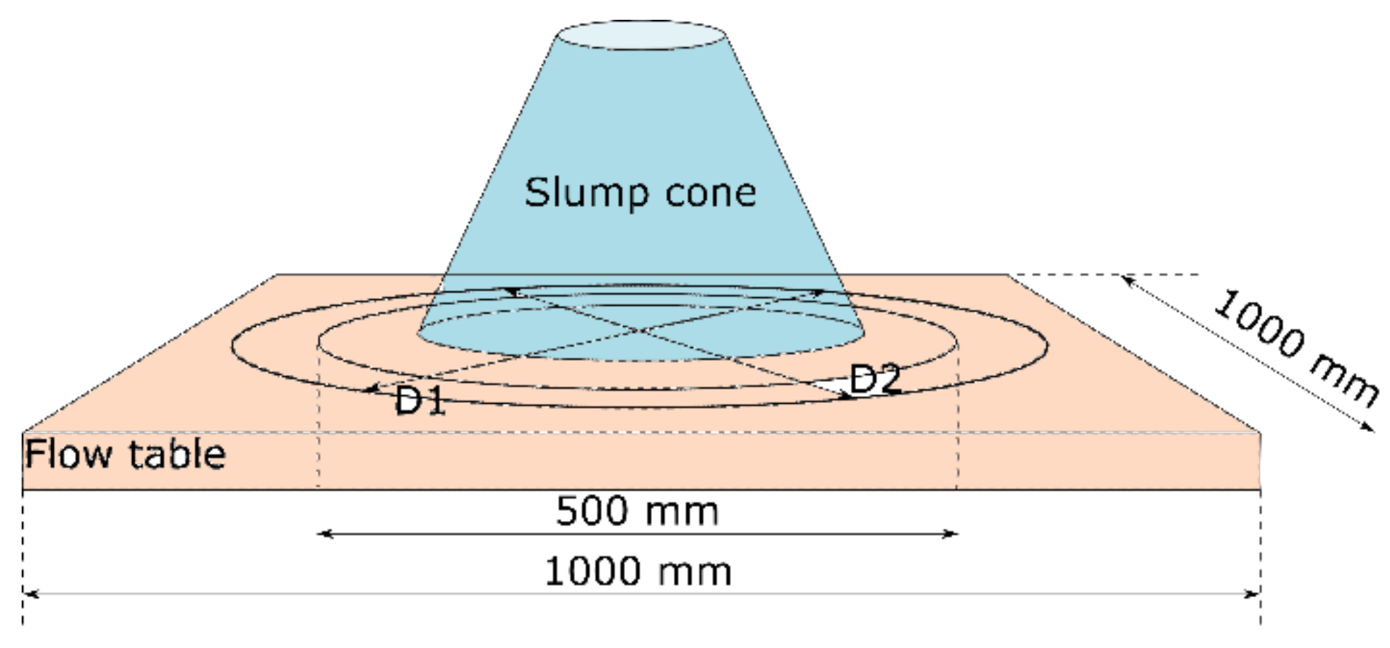
2.1.1. Slump Flow Test
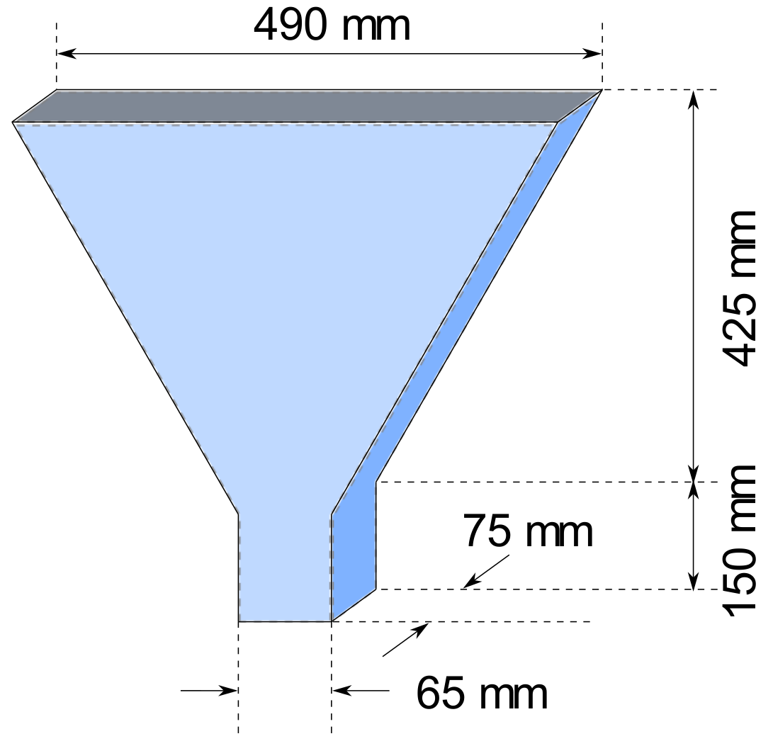
2.1.2. V-Funnel Test
2.1.3. L-Box Test
2.2. Ensemble Machine Learning Process
2.3. Gradient Boosting Algorithms
3. Results
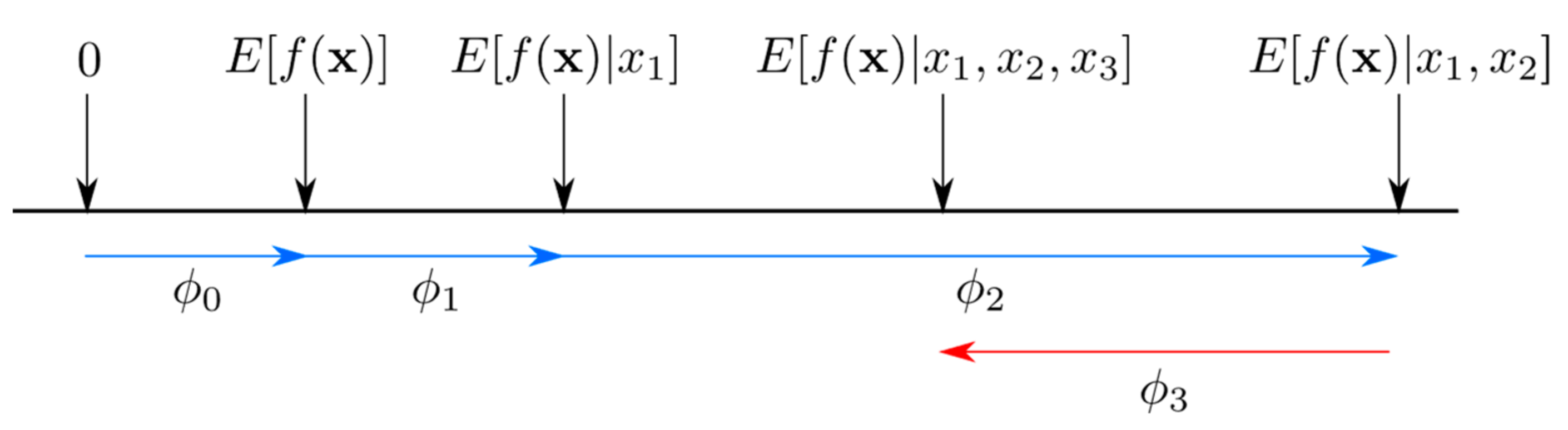
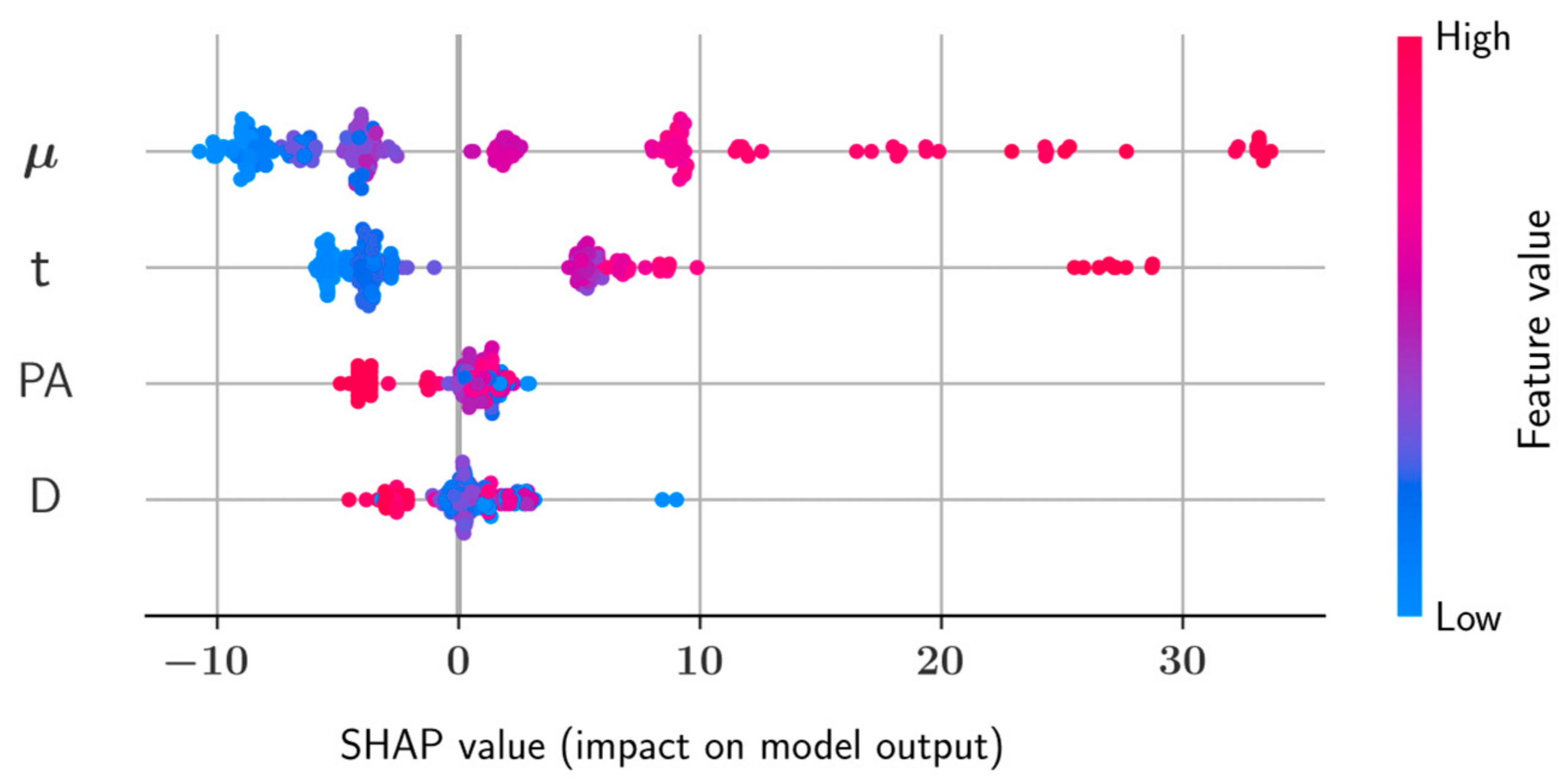
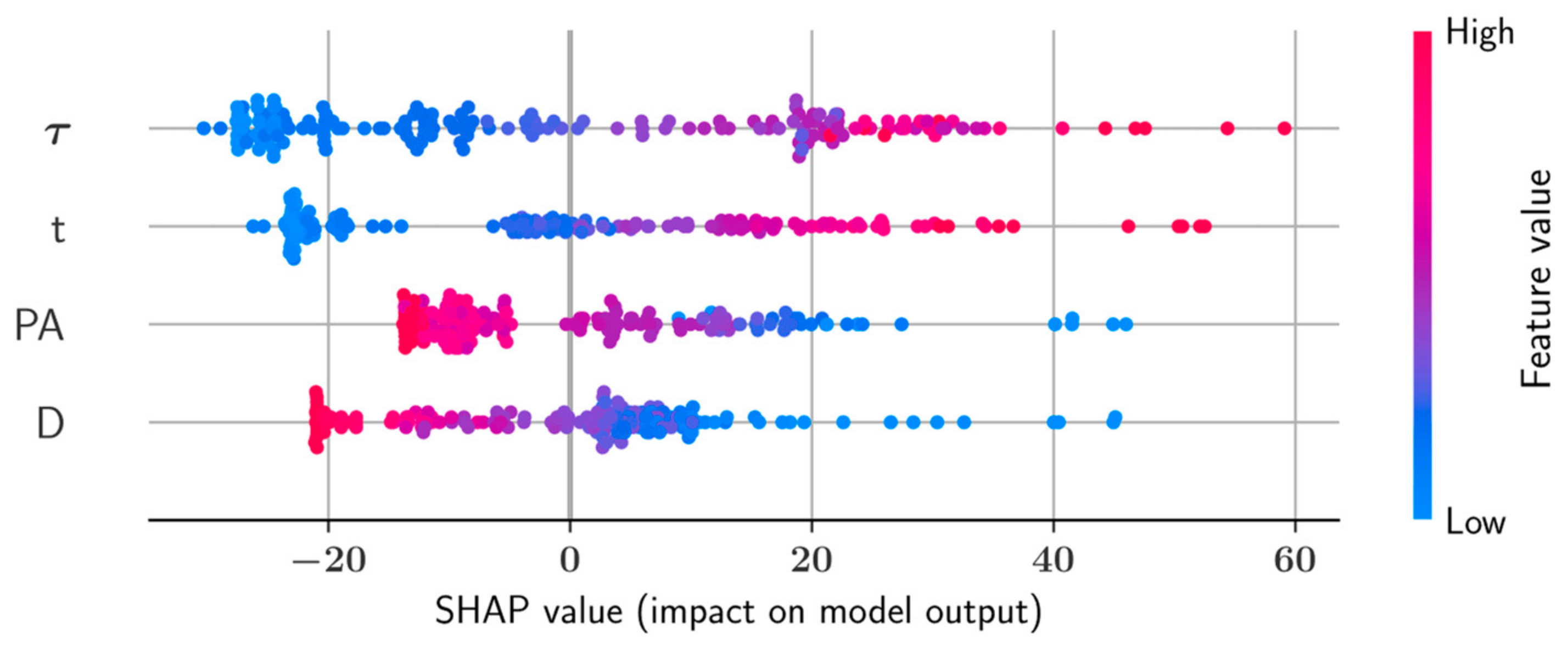
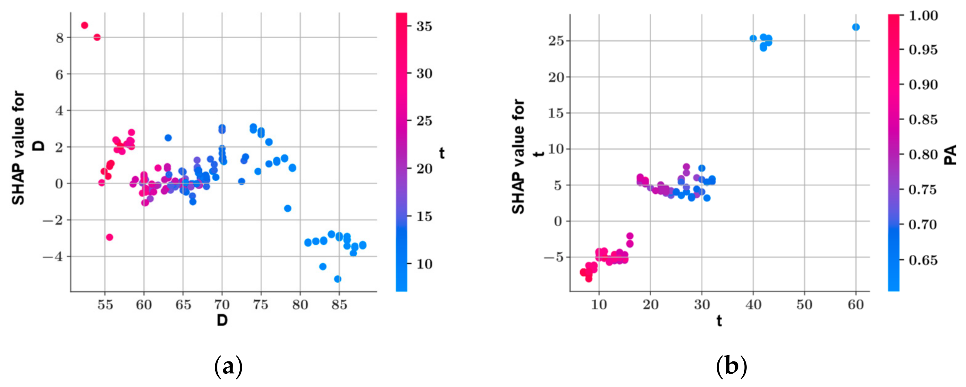
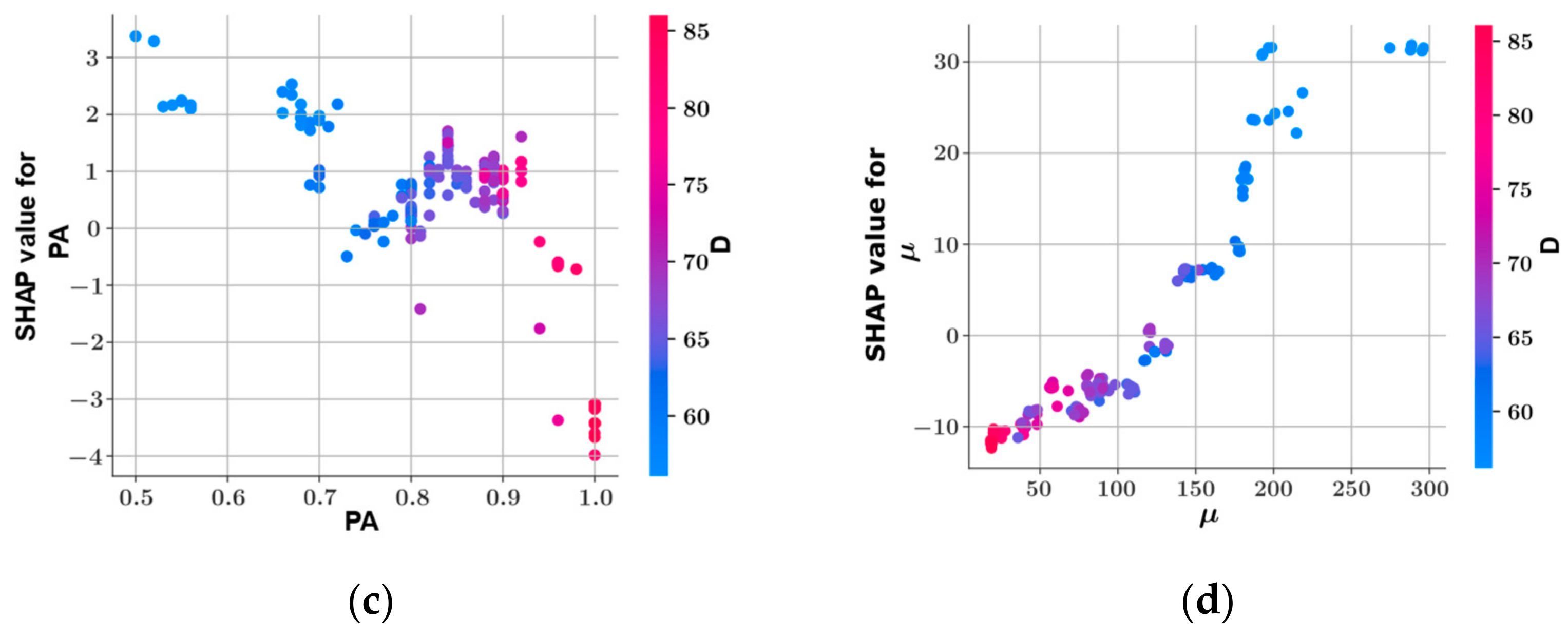
SHAP Analysis
4. Discussion and Conclusions
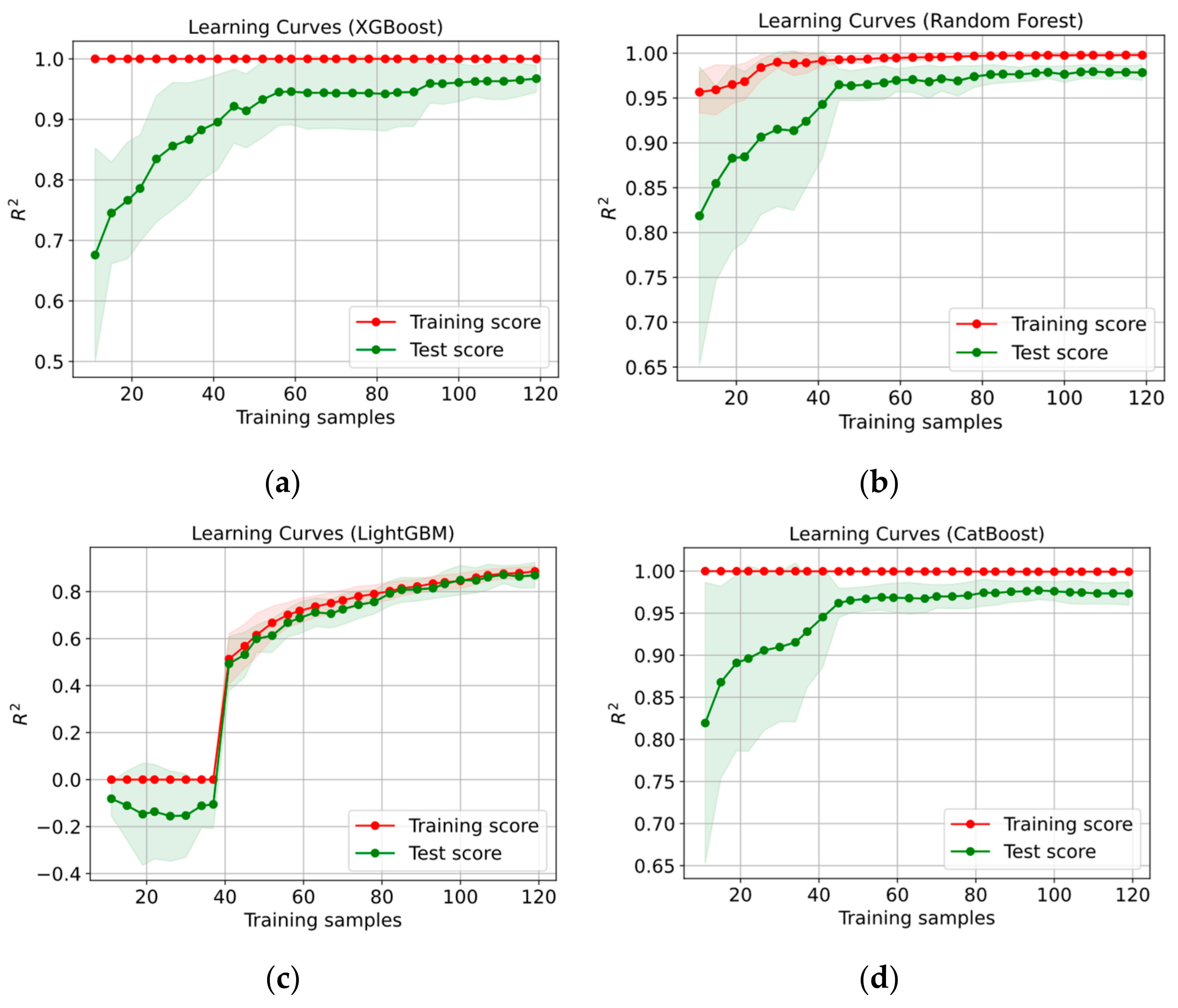
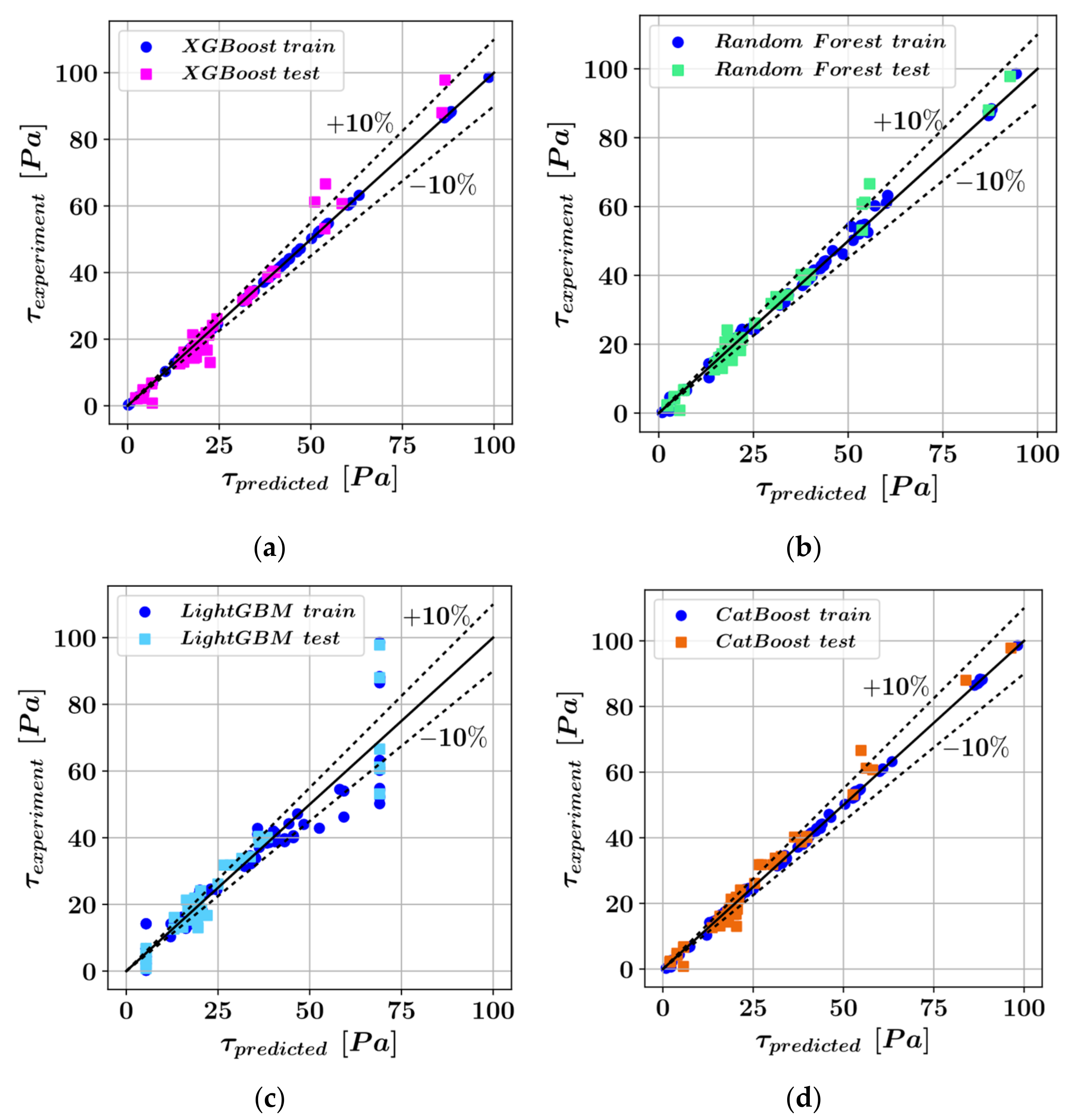
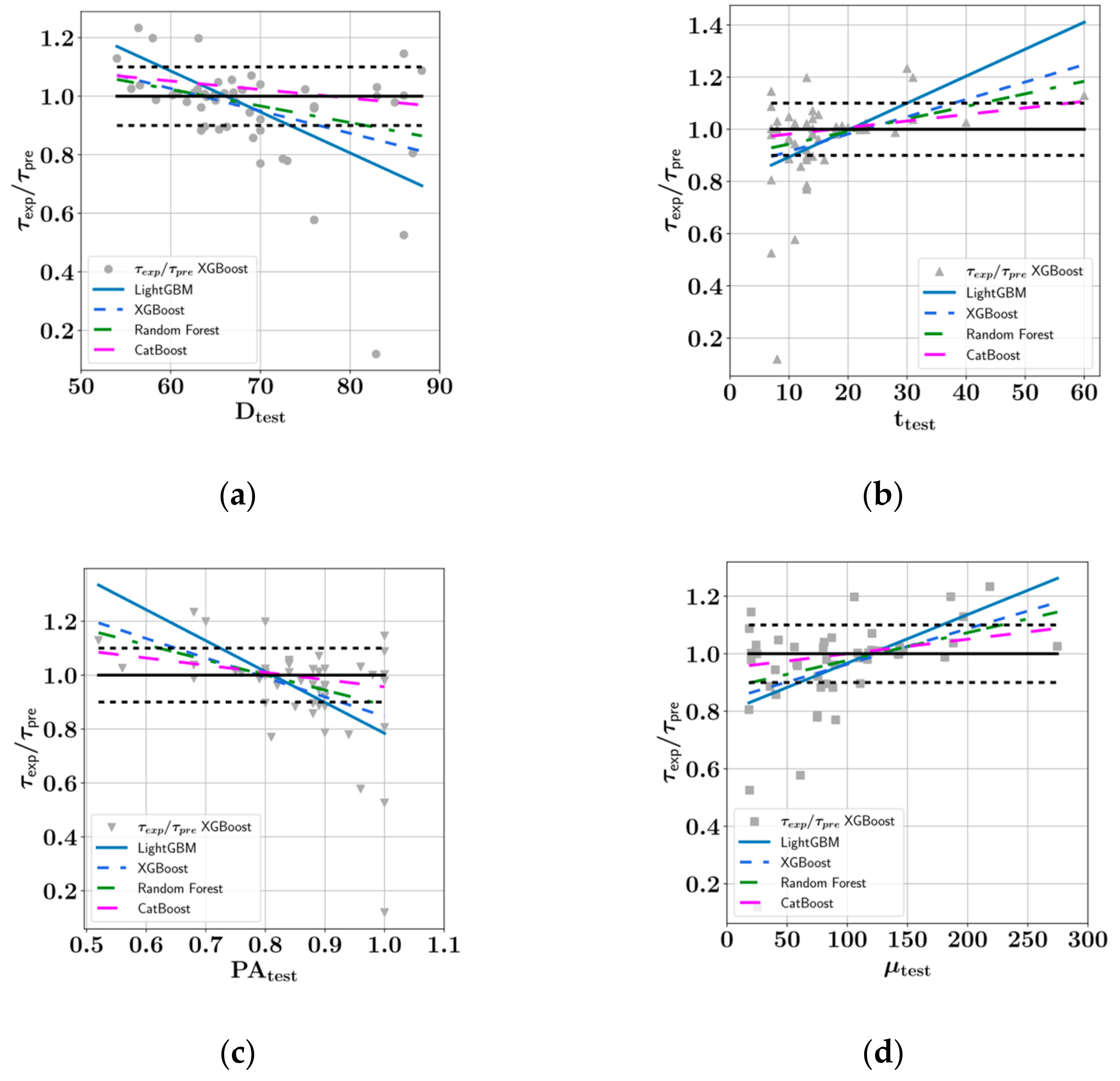
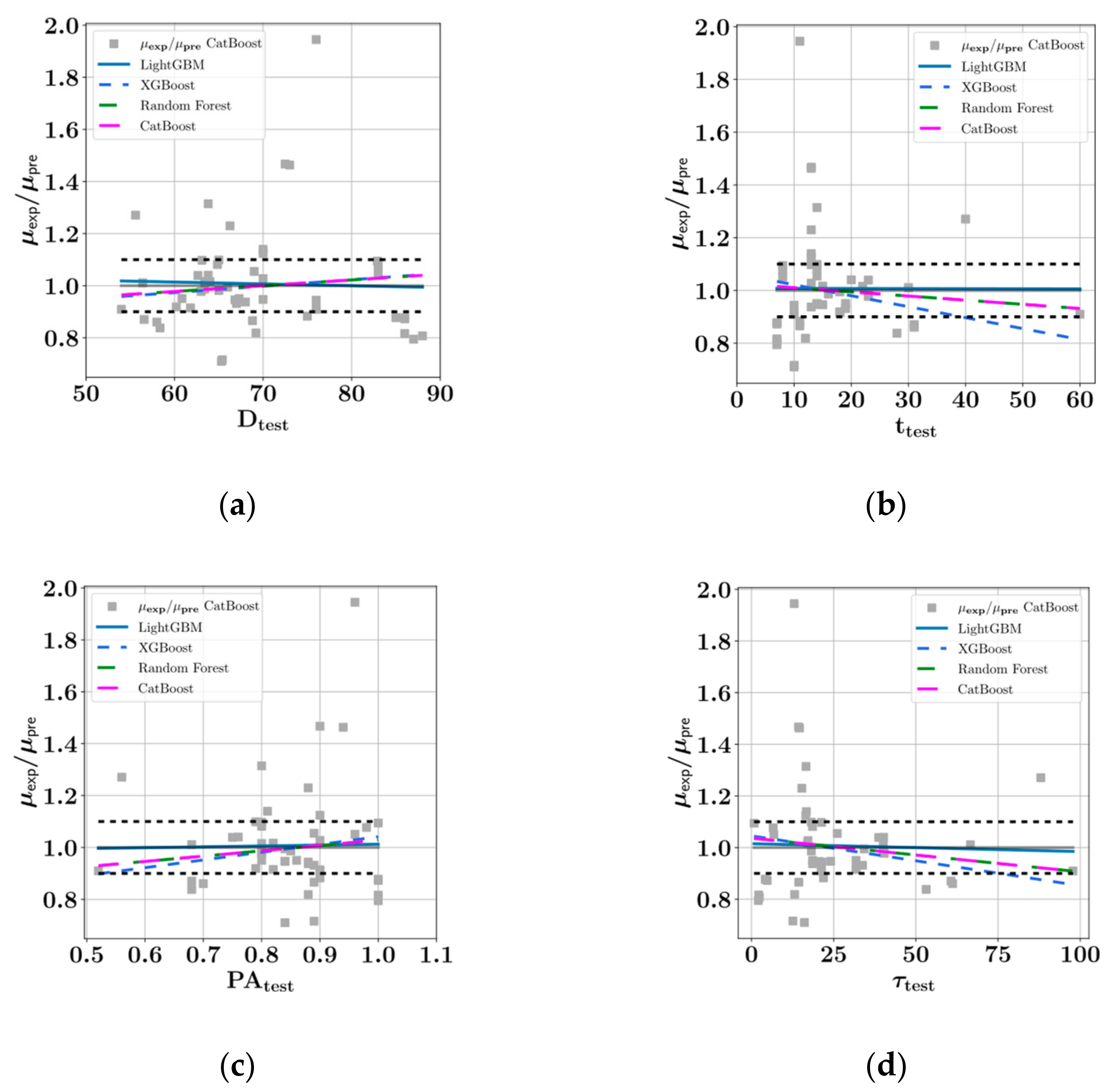
- The XGBoost model performed best on the test set during the prediction of shear stress as a function of the variables D, t, PA, and with an score of 0.9802, followed by random forest ( = 0.9797), CatBoost ( = 0.9779), and LightGBM ( = 0.9111).
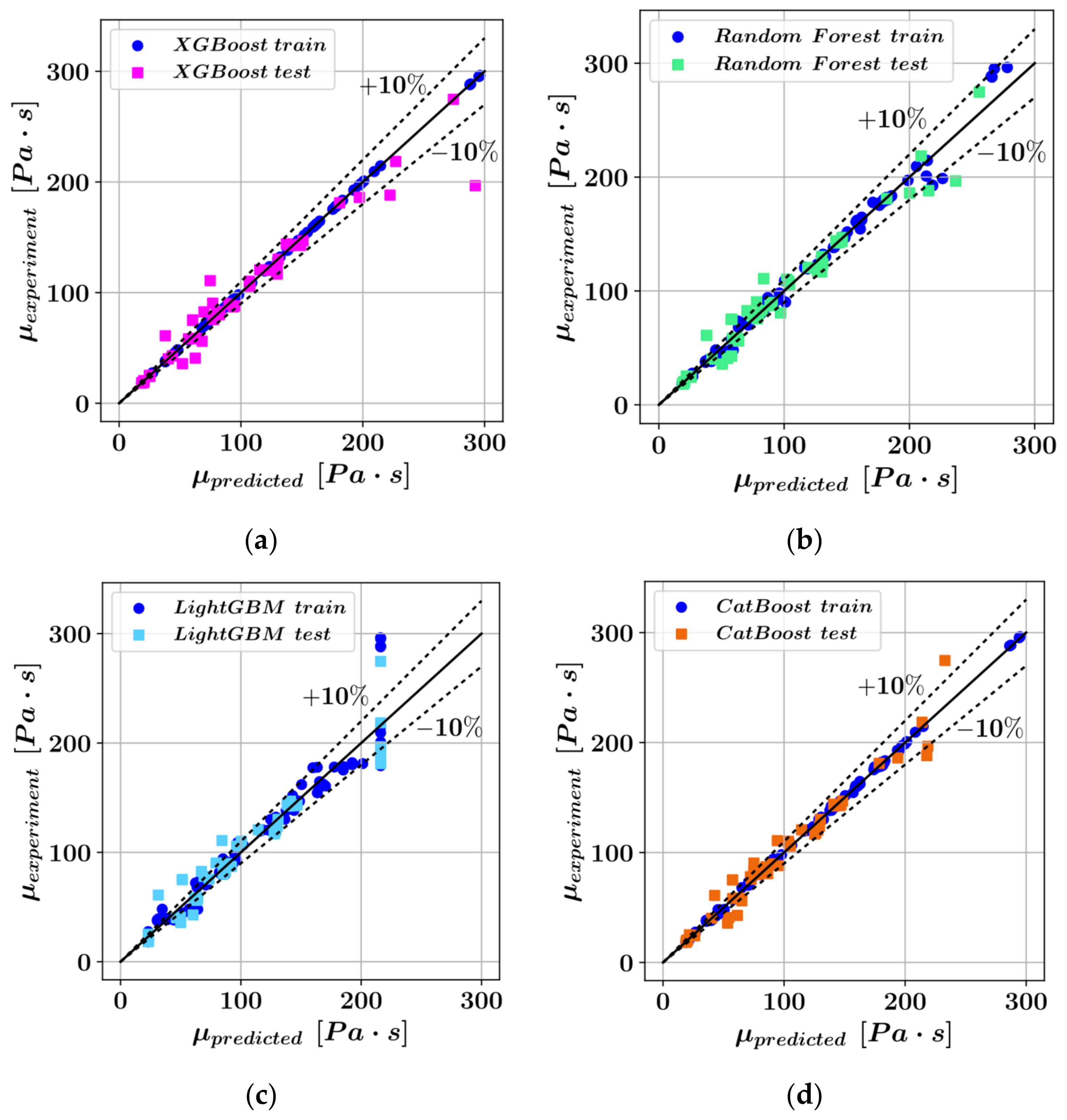
- The CatBoost model performed best on the test set during the prediction of plastic viscosity as a function of D, t, PA, and with an score of 0.9654, followed by random forest ( = 0.9570), LightGBM ( = 0.9387), and XGBoost ( = 0.9132).
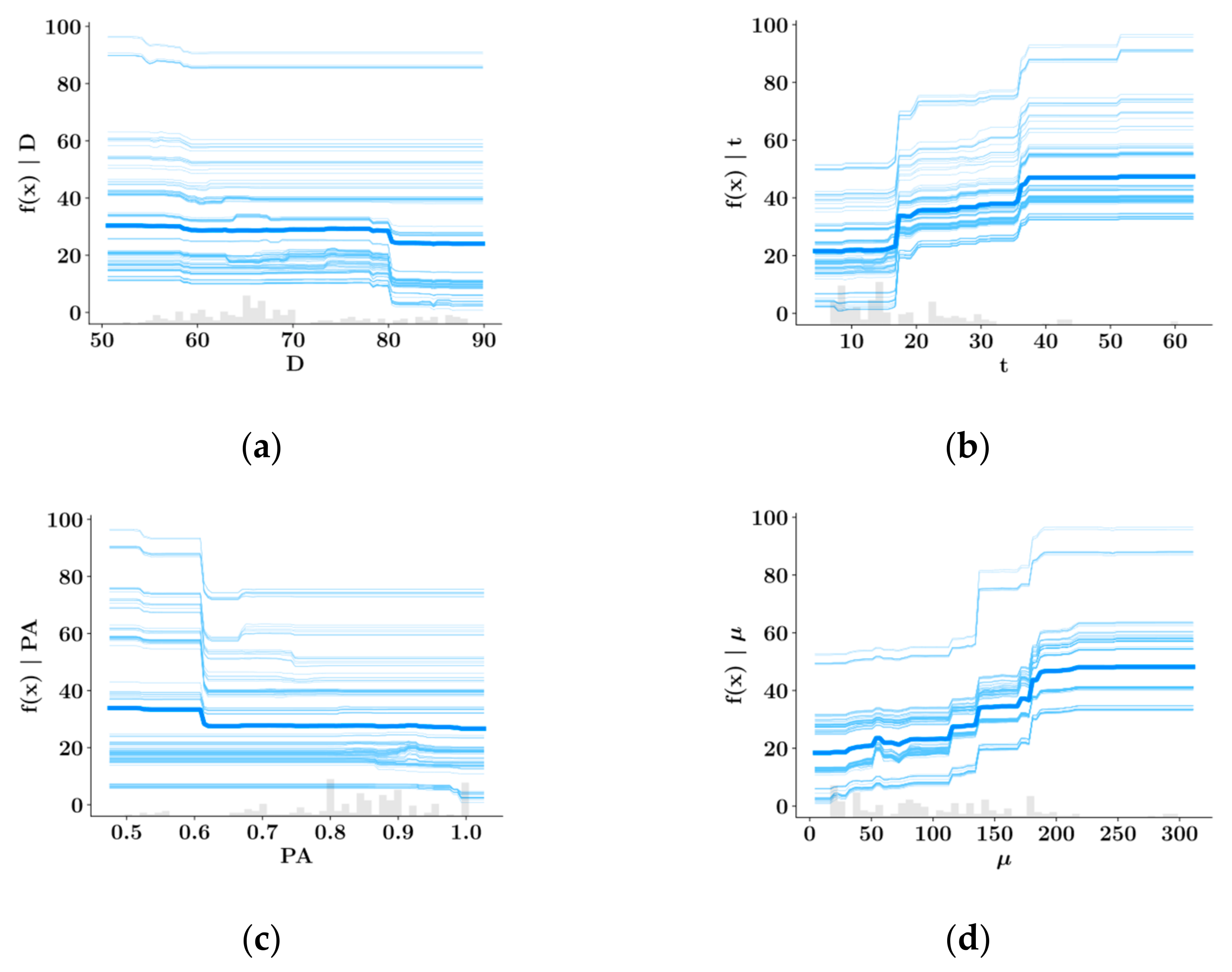
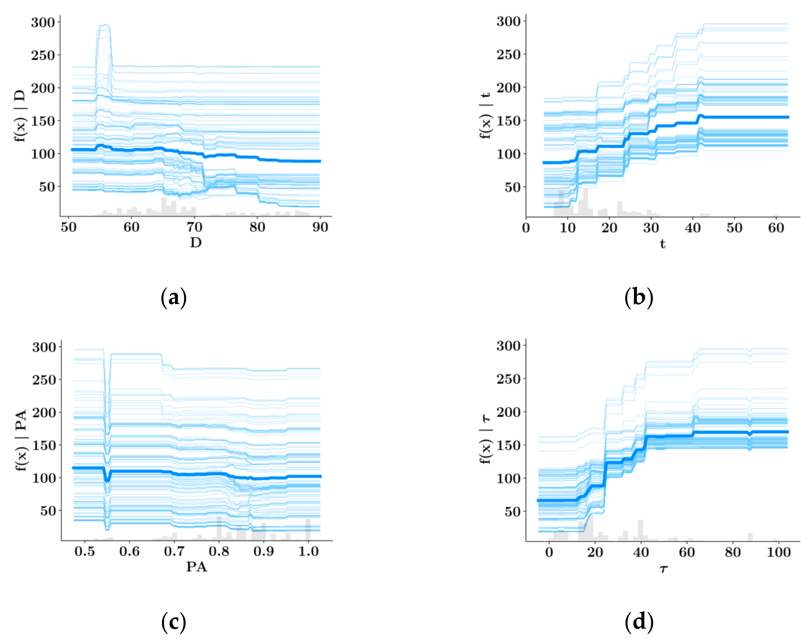
- Shear strength and plastic viscosity features were found to have the highest impact on the predictive model output during prediction of each other, based on the SHAP analysis. In the prediction of both shear stress and plastic viscosity, the slump flow diameter was found to have the lowest impact on the model output.
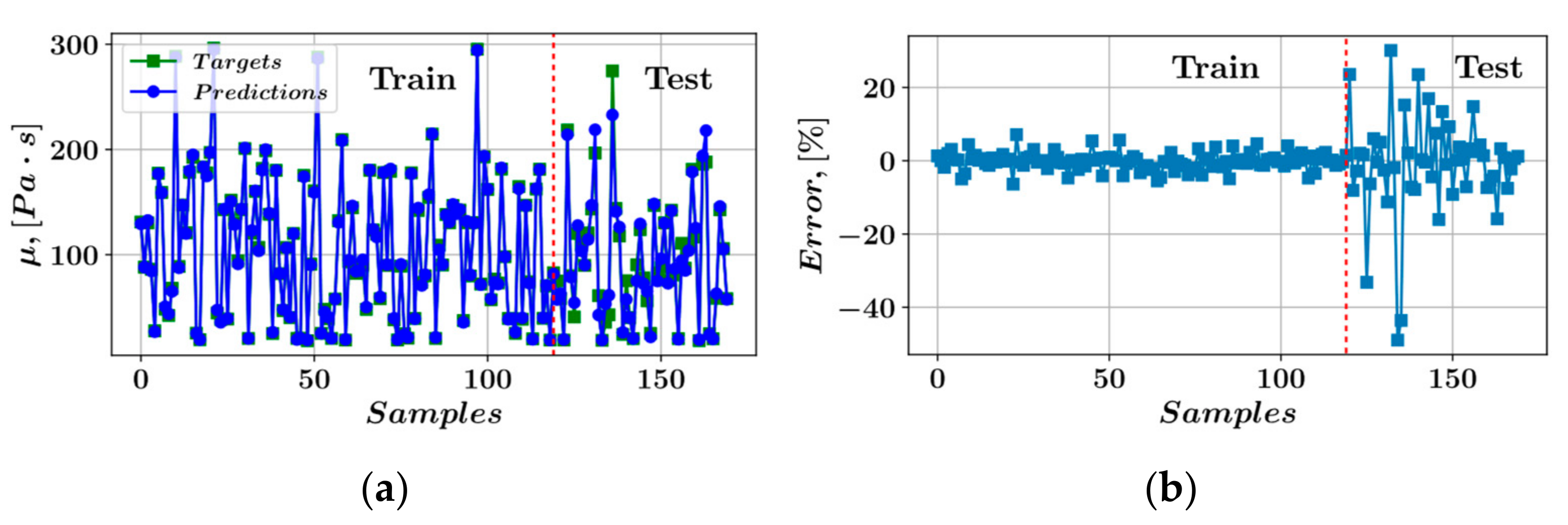
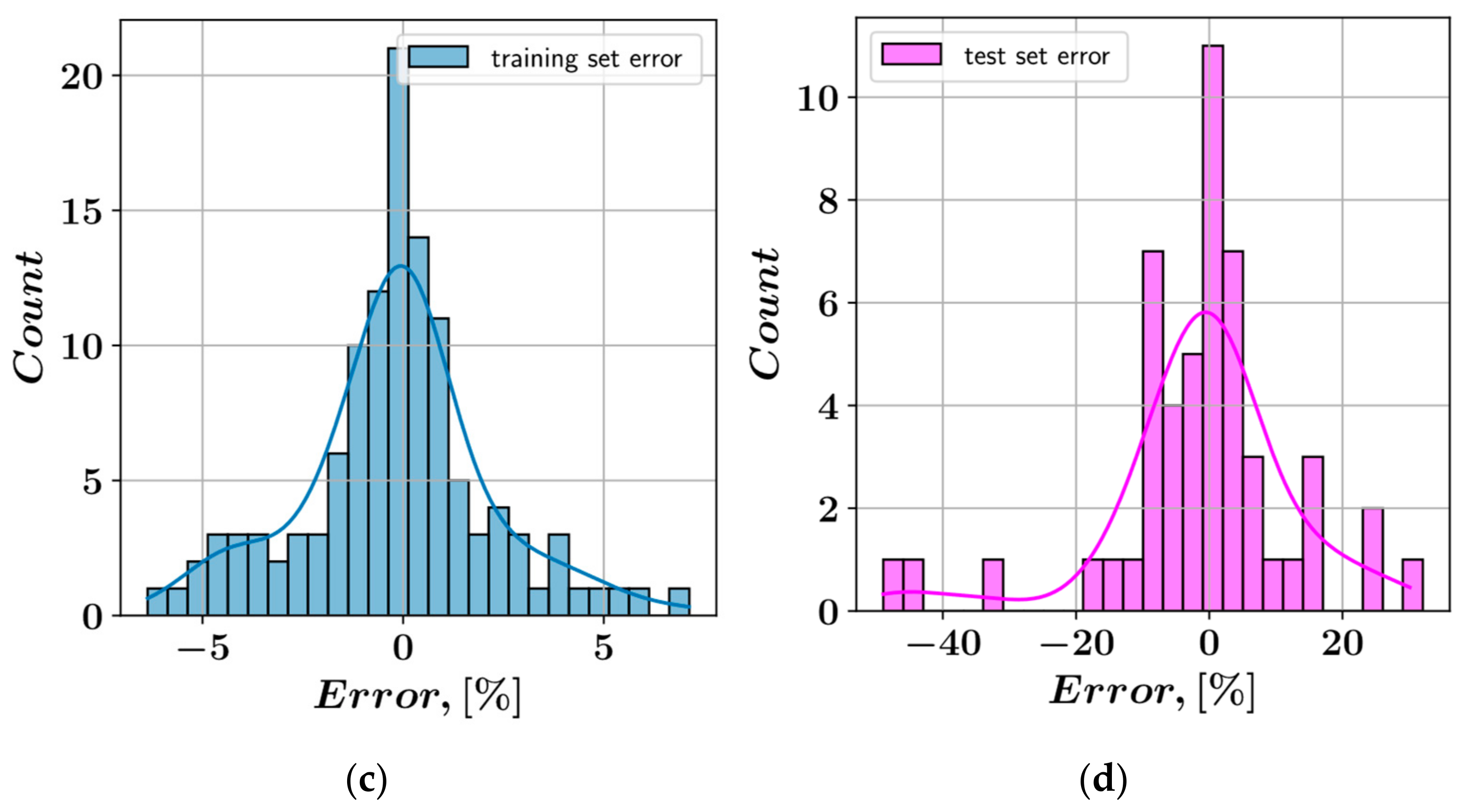
- In the prediction of shear stress, the most consistent predictions were made by the CatBoost model, whereas the LightGBM model was most consistent in predicting plastic viscosity.
Author Contributions
Funding
Data Availability Statement
Conflicts of Interest
References
- Bartos, P.J.M.; Sonebi, M.; Tamimi, A.K. Report of Rilem Technical Committee TC145 WSM, Compendium of Tests, Workability and Rheology of Fresh Concrete; RILEM (The International Union of Testing and Research Laboratories for Materials and Structures): Paris, France, 2002. [Google Scholar]
- Ben Aicha, M.; Burtschell, Y.; Alaoui, A.H.; El Harrouni, K.; Jalbaud, O. Correlation between Bleeding and Rheological Characteristics of Self-Compacting Concrete. J. Mater. Civ. Eng. 2017, 29, 05017001. [Google Scholar] [CrossRef]
- Okamura, H.; Ouchi, M. Self-compacting high performance concrete. Prog. Struct. Eng. Mater. 1998, 1, 378–383. [Google Scholar] [CrossRef]
- Pashias, N.; Boger, D.V.; Summers, J.; Glenister, D.J. A fifty cent rheometer for yield stress measurement. J. Rheol. 1996, 40, 1179–1189. [Google Scholar] [CrossRef]
- Roussel, N. Correlation between Yield Stress and Slump: Comparison between Numerical Simulations and Concrete Rheometers Results. Mater. Struct. 2006, 39, 501–509. [Google Scholar] [CrossRef]
- Neophytou, M.K.A.; Pourgouri, S.; Kanellopoulos, A.D.; Petrou, M.F.; Ioannou, I.; Georgiou, G.; Alexandrou, A. Determination of the rheological parameters of self-compacting concrete matrix using slump flow test. Appl. Rheol. 2010, 20. [Google Scholar] [CrossRef]
- Schowalter, W.R.; Christensen, G. Toward a rationalization of the slump test for fresh concrete: Comparisons of calculations and experiments. J. Rheol. 1998, 42, 865–870. [Google Scholar] [CrossRef]
- Lee, J.H.; Kim, J.H.; Yoon, J.Y. Prediction of the yield stress of concrete considering the thickness of excess paste layer. Constr. Build. Mater. 2018, 173, 411–418. [Google Scholar] [CrossRef]
- Sun, Z.; Feng, D.-C.; Mangalathu, S.; Wang, W.-J.; Su, D. Effectiveness Assessment of TMDs in Bridges under Strong Winds Incorporating Machine-Learning Techniques. J. Perform. Constr. Facil. 2022, 36, 04022036. [Google Scholar] [CrossRef]
- Todorov, B.; Billah, A.M. Post-earthquake seismic capacity estimation of reinforced concrete bridge piers using Machine learning techniques. Structures 2022, 41, 1190–1206. [Google Scholar] [CrossRef]
- Todorov, B.; Billah, A.M. Machine learning driven seismic performance limit state identification for performance-based seismic design of bridge piers. Eng. Struct. 2022, 255, 113919. [Google Scholar] [CrossRef]
- Xu, J.; Feng, D.; Mangalathu, S.; Jeon, J. Data-driven rapid damage evaluation for life-cycle seismic assessment of regional reinforced concrete bridges. Earthq. Eng. Struct. Dyn. 2022, 51, 2730–2751. [Google Scholar] [CrossRef]
- Chen, M.; Mangalathu, S.; Jeon, J.-S. Machine Learning–Based Seismic Reliability Assessment of Bridge Networks. J. Struct. Eng. 2022, 148, 06022002. [Google Scholar] [CrossRef]
- Somala, S.N.; Karthikeyan, K.; Mangalathu, S. Time period estimation of masonry infilled RC frames using machine learning techniques. Structures 2021, 34, 1560–1566. [Google Scholar] [CrossRef]
- Hwang, S.-H.; Mangalathu, S.; Shin, J.; Jeon, J.-S. Estimation of economic seismic loss of steel moment-frame buildings using a machine learning algorithm. Eng. Struct. 2022, 254, 113877. [Google Scholar] [CrossRef]
- Hwang, S.-H.; Mangalathu, S.; Shin, J.; Jeon, J.-S. Machine learning-based approaches for seismic demand and collapse of ductile reinforced concrete building frames. J. Build. Eng. 2020, 34, 101905. [Google Scholar] [CrossRef]
- Moghaddas, S.A.; Nekoei, M.; Golafshani, E.M.; Nehdi, M.; Arashpour, M. Modeling carbonation depth of recycled aggregate concrete using novel automatic regression technique. J. Clean. Prod. 2022, 371, 133522. [Google Scholar] [CrossRef]
- Safayenikoo, H.; Nejati, F.; Nehdi, M.L. Indirect Analysis of Concrete Slump Using Different Metaheuristic-Empowered Neural Processors. Sustainability 2022, 14, 10373. [Google Scholar] [CrossRef]
- Shah, H.A.; Nehdi, M.L.; Khan, M.I.; Akmal, U.; Alabduljabbar, H.; Mohamed, A.; Sheraz, M. Predicting Compressive and Splitting Tensile Strengths of Silica Fume Concrete Using M5P Model Tree Algorithm. Materials 2022, 15, 5436. [Google Scholar] [CrossRef]
- Zhao, G.; Wang, H.; Li, Z. Capillary water absorption values estimation of building stones by ensembled and hybrid SVR models. J. Intell. Fuzzy Syst. 2022, 1–13. [Google Scholar] [CrossRef]
- Benemaran, R.S.; Esmaeili-Falak, M.; Javadi, A. Predicting resilient modulus of flexible pavement foundation using extreme gradient boosting based optimised models. Int. J. Pavement Eng. 2022. [Google Scholar] [CrossRef]
- Bekdaş, G.; Cakiroglu, C.; Kim, S.; Geem, Z.W. Optimization and Predictive Modeling of Reinforced Concrete Circular Columns. Materials 2022, 15, 6624. [Google Scholar] [CrossRef] [PubMed]
- Cakiroglu, C.; Islam, K.; Bekdaş, G.; Kim, S.; Geem, Z.W. Interpretable Machine Learning Algorithms to Predict the Axial Capacity of FRP-Reinforced Concrete Columns. Materials 2022, 15, 2742. [Google Scholar] [CrossRef] [PubMed]
- Cakiroglu, C.; Islam, K.; Bekdaş, G.; Isikdag, U.; Mangalathu, S. Explainable machine learning models for predicting the axial compression capacity of concrete filled steel tubular columns. Constr. Build. Mater. 2022, 356, 129227. [Google Scholar] [CrossRef]
- BEN Aicha, M.; Al Asri, Y.; Zaher, M.; Alaoui, A.H.; Burtschell, Y. Prediction of rheological behavior of self-compacting concrete by multi-variable regression and artificial neural networks. Powder Technol. 2022, 401, 117345. [Google Scholar] [CrossRef]
- Alyamaç, K.E.; Ince, R. A preliminary concrete mix design for SCC with marble powders. Constr. Build. Mater. 2009, 23, 1201–1210. [Google Scholar] [CrossRef]
- Taffese, W. Data-Driven Method for Enhanced Corrosion Assessment of Reinforced Concrete Structures. arXiv 2020, arXiv:2007.01164. [Google Scholar] [CrossRef]
- Yuan, J.; Zhao, M.; Esmaeili-Falak, M. A comparative study on predicting the rapid chloride permeability of self-compacting concrete using meta-heuristic algorithm and artificial intelligence techniques. Struct. Concr. 2022, 23, 753–774. [Google Scholar] [CrossRef]
- Kumar, S.; Rai, B.; Biswas, R.; Samui, P.; Kim, D. Prediction of rapid chloride permeability of self-compacting concrete using Multivariate Adaptive Regression Spline and Minimax Probability Machine Regression. J. Build. Eng. 2020, 32, 101490. [Google Scholar] [CrossRef]
- Ge, D.-M.; Zhao, L.-C.; Esmaeili-Falak, M. Estimation of rapid chloride permeability of SCC using hyperparameters optimized random forest models. J. Sustain. Cem. Mater. 2022, 1–19. [Google Scholar] [CrossRef]
- Amin, M.N.; Raheel, M.; Iqbal, M.; Khan, K.; Qadir, M.G.; Jalal, F.E.; Alabdullah, A.A.; Ajwad, A.; Al-Faiad, M.A.; Abu-Arab, A.M. Prediction of Rapid Chloride Penetration Resistance to Assess the Influence of Affecting Variables on Metakaolin-Based Concrete Using Gene Expression Programming. Materials 2022, 15, 6959. [Google Scholar] [CrossRef]
- Aggarwal, S.; Bhargava, G.; Sihag, P. Prediction of compressive strength of scc-containing metakaolin and rice husk ash using machine learning algorithms. In Computational Technologies in Materials Science; CRC Press: Boca Raton, FL, USA, 2021; pp. 193–205. [Google Scholar] [CrossRef]
- Farooq, F.; Czarnecki, S.; Niewiadomski, P.; Aslam, F.; Alabduljabbar, H.; Ostrowski, K.A.; Śliwa-Wieczorek, K.; Nowobilski, T.; Malazdrewicz, S. A Comparative Study for the Prediction of the Compressive Strength of Self-Compacting Concrete Modified with Fly Ash. Materials 2021, 14, 4934. [Google Scholar] [CrossRef]
- Zhu, Y.; Huang, L.; Zhang, Z.; Bayrami, B. Estimation of splitting tensile strength of modified recycled aggregate concrete using hybrid algorithms. Steel Compos. Struct. 2022, 44, 375–392. [Google Scholar] [CrossRef]
- De-Prado-Gil, J.; Palencia, C.; Jagadesh, P.; Martínez-García, R. A Comparison of Machine Learning Tools That Model the Splitting Tensile Strength of Self-Compacting Recycled Aggregate Concrete. Materials 2022, 15, 4164. [Google Scholar] [CrossRef]
- EFNARC. Specification and Guidelines for Self-Compacting Concrete. 2002. Available online: https://wwwp.feb.unesp.br/pbastos/c.especiais/Efnarc.pdf (accessed on 16 September 2022).
- JSCE, Japan Society of Civil Engineers. Recommendations for Self-Compacting Concrete, Concrete Library of JSCE. 1999, 31. 77p. Available online: http://www.jsce.or.jp/committee/concrete/e/newsletter/newsletter01/recommendation/selfcompact/4.pdf (accessed on 16 September 2022).
- Yang, S.; Zhang, J.; An, X.; Qi, B.; Li, W.; Shen, D.; Li, P.; Lv, M. The Effect of Sand Type on the Rheological Properties of Self-Compacting Mortar. Buildings 2021, 11, 441. [Google Scholar] [CrossRef]
- Sahraoui, M.; Bouziani, T. Effects of fine aggregates types and contents on rheological and fresh properties of SCC. J. Build. Eng. 2019, 26, 100890. [Google Scholar] [CrossRef]
- EL Asri, Y.; Benaicha, M.; Zaher, M.; Alaoui, A.H. Prediction of plastic viscosity and yield stress of self-compacting concrete using machine learning technics. Mater. Today: Proc. 2022, 59, A7–A13. [Google Scholar] [CrossRef]
- Benaicha, M.; Roguiez, X.; Jalbaud, O.; Burtschell, Y.; Alaoui, A.H. Influence of silica fume and viscosity modifying agent on the mechanical and rheological behavior of self compacting concrete. Constr. Build. Mater. 2015, 84, 103–110. [Google Scholar] [CrossRef]
- Rahman, J.; Ahmed, K.S.; Khan, N.I.; Islam, K.; Mangalathu, S. Data-driven shear strength prediction of steel fiber reinforced concrete beams using machine learning approach. Eng. Struct. 2021, 233, 111743. [Google Scholar] [CrossRef]
- Somala, S.N.; Chanda, S.; Karthikeyan, K.; Mangalathu, S. Explainable Machine learning on New Zealand strong motion for PGV and PGA. Structures 2021, 34, 4977–4985. [Google Scholar] [CrossRef]
- Degtyarev, V.; Naser, M. Boosting machines for predicting shear strength of CFS channels with staggered web perforations. Structures 2021, 34, 3391–3403. [Google Scholar] [CrossRef]
- Feng, D.-C.; Cetiner, B.; Kakavand, M.R.A.; Taciroglu, E. Data-Driven Approach to Predict the Plastic Hinge Length of Reinforced Concrete Columns and Its Application. J. Struct. Eng. 2021, 147, 04020332. [Google Scholar] [CrossRef]
- Nguyen, Q.H.; Ly, H.-B.; Ho, L.S.; Al-Ansari, N.; Van Le, H.; Tran, V.Q.; Prakash, I.; Pham, B.T. Influence of Data Splitting on Performance of Machine Learning Models in Prediction of Shear Strength of Soil. Math. Probl. Eng. 2021, 2021, 1–15. [Google Scholar] [CrossRef]
- Bakouregui, A.S.; Mohamed, H.M.; Yahia, A.; Benmokrane, B. Explainable extreme gradient boosting tree-based prediction of load-carrying capacity of FRP-RC columns. Eng. Struct. 2021, 245, 112836. [Google Scholar] [CrossRef]
- Chen, T.; Guestrin, C. Xgboost: A scalable tree boosting system. In Proceedings of the 22nd Acm Sigkdd International Conference on Knowledge Discovery and Data Mining, San Francisco, CA, USA, 13–17 August 2016; pp. 785–794. [Google Scholar]
- Feng, D.-C.; Wang, W.-J.; Mangalathu, S.; Hu, G.; Wu, T. Implementing ensemble learning methods to predict the shear strength of RC deep beams with/without web reinforcements. Eng. Struct. 2021, 235, 111979. [Google Scholar] [CrossRef]
- Ke, G.; Meng, Q.; Finley, T.; Wang, T.; Chen, W.; Ma, W.; Ye, Q.; Liu, T.Y. Lightgbm: A highly efficient gradient boosting decision tree. In Proceedings of the 31st International Conference on Neural Information Processing Systems, Long Beach, CA, USA, 4–9 December 2017; Curran Associates Inc.: New York, NY, USA, 2017. [Google Scholar]
- Prokhorenkova, L.; Gusev, G.; Vorobev, A.; Dorogush, A.V.; Gulin, A. CatBoost: Unbiased boosting with categorical features. In Proceedings of the 32nd International Conference on Neural Information Processing Systems, Montréal, QC, Canada, 3–8 December 2018; Curran Associates Inc.: New York, NY, USA, 2018. [Google Scholar]
- Lundberg, S.M.; Lee, S.-I. A unified approach to interpreting model predictions. In Proceedings of the 31st Conference on Neural Information Processing Systems (NIPS 2017), Long Beach, CA, USA, 4–9 December 2017. [Google Scholar] [CrossRef]
- Mangalathu, S.; Hwang, S.-H.; Jeon, J.-S. Failure mode and effects analysis of RC members based on machine-learning-based SHapley Additive exPlanations (SHAP) approach. Eng. Struct. 2020, 219, 110927. [Google Scholar] [CrossRef]


| Dataset | Property | D | t | PA | ||
|---|---|---|---|---|---|---|
| Training (119 samples) | Unit | cm | s | - | ||
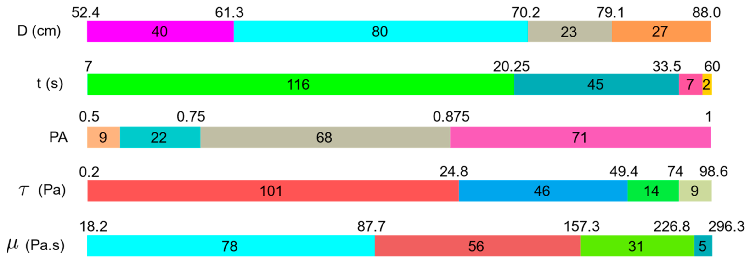
| Min | 52.4 | 7.0 | 0.5 | 18.2 | 0.2 | |
| Max | 88.0 | 60.0 | 1.0 | 296.3 | 98.6 | |
| Mean | 68.19 | 18.10 | 0.83 | 107.40 | 29.23 | |
| SD | 9.08 | 9.94 | 0.11 | 67.34 | 21.54 | |
| As | 0.65 | 1.30 | −0.69 | 0.57 | 1.18 | |
| K | −0.54 | 2.09 | 0.35 | −0.10 | 1.28 | |
| Test (51 samples) | Min | 54.0 | 7.0 | 0.52 | 18.3 | 0.8 |
| Max | 88.0 | 60.0 | 1.0 | 274.65 | 97.8 | |
| Mean | 69.30 | 16.04 | 0.85 | 93.26 | 25.34 | |
| SD | 9.12 | 9.57 | 0.11 | 58.22 | 20.71 | |
| As | 0.59 | 2.38 | −0.83 | 0.81 | 1.63 | |
| K | −0.55 | 7.45 | 0.99 | 0.52 | 2.78 |
| Model | Parameter | Value |
|---|---|---|
| Random Forest | Number of estimators (n_estimators) | 5 |
| Minimum samples for split (min_samples_split) | 3 | |
| Minimum samples of leaf node (min_samples_leaf) | 1 | |
| Maximum tree depth (max_depth) | None | |
| Number of features (max_features) | “sqrt” | |
| XGBoost | Number of estimators (n_estimators) | 50 |
| Step size shrinkage (eta) | 0 | |
| Learning rate | 0.1 | |
| Subsample ratio of the training instances (subsample) | 0.5 | |
| Maximum depth of a tree | 6 | |
| LightGBM | Number of estimators (n_estimators) | 500 |
| Maximum number of decision leaves (num_leaves) | 5 | |
| Maximum depth of a tree (max_depth) | 4 | |
| Learning rate | 0.2 | |
| use extremely randomized trees (extra_trees) | True | |
| CatBoost | Bagging temperature (bagging_temperature) | 10 |
| Learning rate | 0.3 | |
| Depth | 8 | |
| Tree growing policy (grow_policy) | “Depthwise” |
| Algorithm | R2 | MAE | VAF | RMSE | Duration [s] | ||||
|---|---|---|---|---|---|---|---|---|---|
| Train | Test | Train | Test | Train | Test | Train | Test | ||
| XGBoost | 0.9997 | 0.9802 | 0.094 | 1.712 | 99.99 | 97.04 | 0.397 | 2.885 | 4.54 |
| Random Forest | 0.9977 | 0.9797 | 0.658 | 1.795 | 99.76 | 98.05 | 1.037 | 2.924 | 3.24 |
| LightGBM | 0.8968 | 0.9111 | 4.104 | 3.624 | 90.08 | 90.80 | 6.888 | 6.114 | 4.04 |
| CatBoost | 0.9988 | 0.9779 | 0.572 | 2.120 | 99.92 | 97.98 | 0.747 | 3.047 | 22.69 |
| Algorithm | R2 | MAE | VAF | RMSE | Duration [s] | ||||
|---|---|---|---|---|---|---|---|---|---|
| Train | Test | Train | Test | Train | Test | Train | Test | ||
| XGBoost | 0.9999 | 0.9132 | 0.041 | 8.274 | 99.99 | 91.56 | 0.084 | 16.986 | 4.66 |
| Random Forest | 0.9896 | 0.9570 | 3.665 | 7.703 | 98.74 | 95.44 | 6.846 | 11.961 | 3.15 |
| LightGBM | 0.9324 | 0.9387 | 9.527 | 9.286 | 93.61 | 93.18 | 17.437 | 14.270 | 3.65 |
| CatBoost | 0.9986 | 0.9654 | 1.764 | 7.602 | 99.95 | 96.32 | 2.487 | 10.727 | 19.82 |
Publisher’s Note: MDPI stays neutral with regard to jurisdictional claims in published maps and institutional affiliations. |
© 2022 by the authors. Licensee MDPI, Basel, Switzerland. This article is an open access article distributed under the terms and conditions of the Creative Commons Attribution (CC BY) license (https://creativecommons.org/licenses/by/4.0/).
Share and Cite
Cakiroglu, C.; Bekdaş, G.; Kim, S.; Geem, Z.W. Explainable Ensemble Learning Models for the Rheological Properties of Self-Compacting Concrete. Sustainability 2022, 14, 14640. https://doi.org/10.3390/su142114640
Cakiroglu C, Bekdaş G, Kim S, Geem ZW. Explainable Ensemble Learning Models for the Rheological Properties of Self-Compacting Concrete. Sustainability. 2022; 14(21):14640. https://doi.org/10.3390/su142114640
Chicago/Turabian StyleCakiroglu, Celal, Gebrail Bekdaş, Sanghun Kim, and Zong Woo Geem. 2022. "Explainable Ensemble Learning Models for the Rheological Properties of Self-Compacting Concrete" Sustainability 14, no. 21: 14640. https://doi.org/10.3390/su142114640
APA StyleCakiroglu, C., Bekdaş, G., Kim, S., & Geem, Z. W. (2022). Explainable Ensemble Learning Models for the Rheological Properties of Self-Compacting Concrete. Sustainability, 14(21), 14640. https://doi.org/10.3390/su142114640