Abstract
Indoor occupancy prediction can play a vital role in the energy-efficient operation of building engineering systems and maintaining satisfactory indoor climate conditions at the lowest possible energy use by operating these systems on the basis of occupancy data. Many methods have been proposed to predict occupancy in residential buildings according to different data types, e.g., digital cameras, motion sensors, and indoor climate sensors. Among these proposed methods, those with indoor climate data as input have received significant interest due to their less intrusive and cost-effective approach. This paper proposes a deep learning method called CNN-XGBoost to predict occupancy using indoor climate data and compares the performance of the proposed method with a range of supervised and unsupervised machine learning algorithms plus artificial neural network algorithms. The comparison is performed using mean absolute error, confusion matrix, and F1 score. Indoor climate data used in this work are CO2, relative humidity, and temperature measured by sensors for 13 days in December 2021. We used inexpensive sensors in different rooms of a residential building with a balanced mechanical ventilation system located in northwest Copenhagen, Denmark. The proposed algorithm consists of two parts: a convolutional neural network that learns the features of the input data and a scalable end-to-end tree-boosting classifier. The result indicates that CNN-XGBoost outperforms other algorithms in predicting occupancy levels in all rooms of the test building. In this experiment, we achieved the highest accuracy in occupancy detection using inexpensive indoor climate sensors in a mechanically ventilated residential building with minimum privacy invasion.
1. Introduction
Residential buildings use a considerable amount of energy such that, according to Eurostat, in 2020, households represented 28% of the total energy used in the EU [1]. This study also reported that space heating and cooling have the highest energy use in households in the EU (2020), i.e., 63.2% of the total energy use in the residential sector [2]. One of the consequences of world population growth is the increase in residential houses and energy consumption. Therefore, the need for modern technologies is growing to reduce occupant-related energy consumption.
When it comes to occupants’ behavior, several studies have shown that the amount of energy demanded by buildings can vary due to occupants’ behavior, i.e., occupants’ presence, the number of occupants, and their preferred thermal comfort [3,4,5].
Occupants have a significant role in reducing energy use. Therefore, to save energy, a possible method is to detect occupants using cameras, Wi-Fi, Bluetooth, PIR sensors, light sensors, RFIDs, and indoor climate sensors (e.g., temperature, relative humidity, and CO2), as well as to configure the heating, ventilation, and air conditioning (HVAC) system using data from the occupants’ presence [6,7,8,9,10,11,12,13]. Studies have shown that using occupancy detection can save up to 60% in HVAC energy use [13,14,15].
1.1. Related Works
Many studies have been conducted to detect occupancy levels. These methods can be divided into four major categories: traditional statistical methods, unsupervised machine learning methods, supervised machine learning methods, and hybrid machine learning methods.
Most of the models applied in traditional statistical models are Markov chain-based models [16,17,18]. To predict occupancy at the binary level and the number of occupants for the offices located in the US, Li and Dong [19] proposed a Makov model including change-point analysis with a moving window training and a modified random sampling approach. These methods are compared with two simulation models (Page’s Markov and Reinhart’s Lightswitch) and two machine learning methods (artificial neutral network (ANN) and SV regression). They tested the predictive accuracy of the approaches in forecasting the presence and number of occupants 15 min, 30 min, and 24 h ahead. The results showed that the proposed Markov-based model outperformed the other four methods. Huang et al. [20] used a Wi-Fi indoor positioning system to predict occupancy levels as a function of dwell time distribution. They studied passenger flow at Shanghai Hongqiao International Airport for 66 days. They modeled the distribution of passengers’ dwell time using a Bayesian method. They predicted occupancy levels with a relative r-square of 0.747. Pedersen et al. [21] proposed an occupancy prediction method called plug-and-play which follows the trajectory of indoor climate sensors data to calculate the probability of occupancy according to a set of defined rules. This probability is then converted into an unoccupied/occupied binary signal with a user-defined threshold. They used indoor climate parameters CO2, air temperature, and humidity, in addition to passive infrared (PIR), noise, and volatile organic compounds (VOCs) in a simple test room and a residential apartment with three bedrooms. In the test room, the results showed that the occupancy prediction based on the CO2 measurements had the minimum mean absolute error, in comparison with the results obtained from the measurements of the other sensors. In the apartment, the occupancy prediction based on the measurements of the PIR sensor gave the most accurate occupancy prediction when the apartment went from unoccupied to occupied, while occupancy prediction based on measurements of the VOC or CO2 sensors gave the most accurate occupancy prediction when the apartment went from occupied to unoccupied.
In today’s occupancy prediction literature, the use of ML methods is growing due to their flexibility and accuracy in predicting occupancy either as a binary or according to the number of occupants. To implement a prediction model utilizing machine learning methods for residential buildings, we should pay attention to many principal subjects, i.e., occupants’ privacy, occupancy prediction accuracy, method implementation cost, method complexity, speed of the method, etc. Dai et al. [22] reviewed the studies applying machine learning (ML) methods to predict occupancy and window-opening behaviors in smart buildings.
Generally, ML algorithms are divided into supervised and unsupervised algorithms. Unsupervised learning is a machine learning technique in which a model tries to cluster untagged data. The goal of clustering is to find natural grouping relations in data and discover if a data point belongs to a cluster or not. Examples of these algorithms are k-means clustering and principal component analysis. Killian and Kozek [23] proposed a model predictive control for smart homes using an unsupervised occupancy prediction method. They combined the proper orthogonal decomposition [24] with KMC, which is capable of using the full power of energy storage in a smart home with almost the same comfort.
Supervised learning is a machine learning technique in that the model has input data connected with a specific output. Examples of supervised algorithms are KNN, SV, GB, RF, linear regression, LR, DT, neural networks (NNs), and naïve Bayes. KNN has been used to identify the presence, number, and location of the occupants using motion sensors and RFID technology [25,26].
Aftab et el. [27] developed an automatic HVAC controller in a public mosque. This controller can predict occupancy levels using linear regression. The study used a method based on a Raspberry Pi 3 platform and a fish-eye camera to track occupancy. The analysis showed that the method had a detection accuracy of 90% in real time and 85% accuracy in occupancy forecast. Using the proposed model would enable building owners to save 20% energy savings while maintaining the comfort of occupants. Privacy invasion is one of the obstacles to implementing camera-based models in residential buildings. Razavi et al. [28] applied some supervised algorithms such as GB, RF, SVM, NN, and KNN to detect the occupancy of residential buildings using smart meter data. The authors concluded that GB with a cross-validation accuracy of 0.982 and precision of 0.997 outperformed the other methods. To forecast occupancy levels in two university laboratories, Mamidi et al. [29] used motion detection, CO2 reading, sound level, ambient light, and door state sensors. They applied several ML and ANN methods: ensemble learning, LR, SVM, and multilayer perceptron (MLP) to predict occupancy levels. The authors concluded that MLP outperformed the other methods in terms of prediction accuracy. To forecast the number of occupants of a test room using an RF classifier, Sangogboye et al. [30] employed common sensors (e.g., temperature, CO2, and PIR) and dedicated sensors (e.g., 3D stereovision camera) separately. The method with common sensors was called GAKF, and the method with dedicated sensors was called CAM. The result showed a normalized mean squared prediction error of 2.972 and 6.57 for CAM and GAKF, respectively, considering that implementing the CAM method costs more than the GAKF method because 3D stereovision cameras are much more expensive than temperature and CO2 sensors. Kampezidou [31] proposed an approach including a physics-informed pattern-recognition machine (PIPRM) to predict binary occupancy in a 3.6 m × 3.6 m × 2.7 m residential room using CO2 and temperature sensor measurements placed on a stand at 50 cm height, away from occupants. Data were collected for 7 days in March, April, and May at different hours. Their model showed the capability of predicting real-time occupancy with an accuracy and an F1 score of 97% and 92.3%, respectively, on test data.
More complicated neural network methods can be found in Kim et al. [32] to cope with the problem of occupancy prediction in large exhibition halls. They proposed spatial partitioning of large exhibition halls and an occupancy prediction model based on a long short-term memory (LSTM) recurrent neural network. They tested their proposed model in a 126 m × 90 m exhibition hall in Goyang, South Korea. They divided the hall into multiple zones and recorded the occupancy using 50 image sensors for 10 days in July 2018. They compared their model with autoregressive integrated moving average (ARIMA) and Holt–Winters models used to predict occupancy in large exhibition halls. The result indicated that ARIMA and Holt–Winters models only showed good performance in short-term (15 min) occupancy prediction, but their model was effective and stable in both short-term and long-term (180 min) occupancy prediction. A neural network learns a person’s behavior and predicts it. This network is unable to predict another person’s behavior accurately. To cope with this problem, Leeraksakiat and Pora [33] applied LSTM to enhance the power of the network when a person occupies a place or changes their comfort, or when a new person enters the place. First, they used a norm dataset to train the network, and then new batches of sampling data were added to update the network, i.e., transferring new knowledge to the previous information. They showed that transfer learning could increase the power of the network to recognize the behavior changes of the occupants.
Compared to other machine learning methods, hybrid method applications are somewhat limited [16]. Hybrid methods are combinations of supervised and unsupervised methods. Sama et al. [34] examined a compression-based sequential prediction approach, based on the Active LeZi algorithm, to predict the occupancy and movement of smart home residents for automation applications. They used motion detector sensors to test their model. Liang et al. [35] worked on the problem of occupancy pattern learning and occupancy schedule prediction in office buildings. Their hybrid approach first recognizes the occupants’ presence patterns using cluster analysis and then learns the schedule rules using the decision tree. The final step is to predict occupancy schedules. They tested their approach using 1 year data related to an office building in Philadelphia, US. The input data were the time-series data of people entering and exiting the building. Validation results showed that the approach had a remarkable improvement in the accuracy of occupancy schedule prediction. Nacer et al. [36] proposed a method called automatic learning of an occupancy schedule (ALOS). Their method was a combination of two parts: an unsupervised clustering method to classify leaving and coming of the occupants in a family residential building consisting of four occupants and a building with one elderly person living alone; a mixture model to determine the doweling time of the occupants. This method was introduced to predict the occupancy of residential buildings to manage the heating system. They installed PIR sensors, CO2 detectors, sound-level meters, hygrometers, and thermometers in their work. The results of their research showed that ALOS could achieve up to 90% accuracy in predicting occupancy.
1.2. Research Gap and Contribution
In occupancy detection, several factors including the accuracy of the model, privacy of occupants, speed of the model, ease of model implementation, and model implementation cost should be considered. Camera-based models are among the most accurate existing models, but they are relatively expensive and invade the residents’ privacy [37]. Wi-Fi and Bluetooth-based models suffer from two issues; occupants need to always carry their smartphone with Bluetooth or Wi-Fi turned on. Moreover, the implementation of these models demands additional costs and maintenance [38]. PIR sensors are unreliable because, when the occupants stay still and motionless, these sensors may log misleading occupancy information [39]. RFIDs are intrusive tags that residents should always take with them. If one of the residents or guests does not take one of these tags, their presence in the environment is not recorded [38]. In general, RFIDs are more suitable for offices than residential buildings.
Most existing research studies were based on prediction models requiring indoor climate data as input. Indoor climate sensors are relatively inexpensive, usually available in existing modern buildings, and easy to implement; however, to compensate for their low prediction accuracy, more complicated models such as ML models are needed [38]. These inexpensive indoor climate sensors are also increasingly available in today’s smart homes. Despite the great potential for energy saving with occupancy detection in residential buildings, little research has been conducted on residential buildings [40,41]. In comparison with office buildings, occupancy detection in residential buildings is more challenging due to the rather low number of occupants and the difficulty in collecting ground-truth data without privacy violations. On the other hand, the implementation of mechanical ventilation systems has been increasing in residential buildings. Occupancy prediction based on indoor climate data is particularly challenging in residential buildings with a mechanical ventilation system since CO2, temperature, and humidity are controlled by the ventilation system to be within certain limits. Interference of the mechanical ventilation system in indoor air causes the accuracy of the model to decrease; hence, the power of the model should be increased.
This literature review revealed a significant contribution of existing research in the advancement of occupancy prediction, but a gap remains with regard to the existence of a fast, cost-effective, and accurate method without violating the privacy of occupants in residential buildings with a balanced mechanical ventilation system. A few studies addressed occupancy detection in residential buildings with a balanced mechanical ventilation system, but most of them did not consider real-life situations. Among the few studies, the work in [31] evaluated the proposed occupancy detection method in a residential building with a mechanical ventilation system. However, the experimental procedure was rather simple, in which only one room in a residential building was considered. The study [42] evaluated a methodology for occupancy detection based on hidden Markov models for different rooms in a passive residential house with a mechanical ventilation system. However, this study only evaluated average daily and hourly occupancy estimation. Likewise, the study in [21] evaluated the occupancy detection method in a three-room dorm apartment with a mechanical ventilation system. However, in this study, the sensor data were only logged at the apartment level, which lowered the accuracy of occupancy detection at the room level. To the authors’ best knowledge, no study in the existing literature has evaluated an indoor climate-based occupancy detection method at room level in a residential building equipped with balanced mechanical ventilation, in which several rooms with different occupancy patterns have been tested.
To fill this gap, we propose an approach that is inexpensive, accurate, easy to install, and fast. In this work, we apply CNN-XGBoost to predict the occupancy in rooms of a residential building using purely indoor climate measurements. Compared to the previous studies conducted in residential buildings with mechanical ventilation, this model extracts the features from indoor climate data to achieve the highest accuracy using inexpensive sensors. The proposed model consists of a convolutional neural network that extracts features of indoor climate data and performs the classification operation with a robust classifier. The main contributions of this work are as follows:
- We experimentally evaluate an ML method to accurately detect occupancy in several rooms with different occupancy patterns in a residential household equipped with a balanced mechanical ventilation system, while, with the least privacy invasion, we impose no limitation on the occupants in using the HVAC system, doors, and windows.
- We propose a novel ML model for occupancy prediction in residential buildings that is fast and sufficiently accurate. The model fills the lack of feature extraction in previous models used in residential buildings with a mechanical ventilation system.
2. Materials and Methods
The present study employs the accuracy and feature extraction capability of convolutional neural networks and the speed, accuracy, and flexibility of XGBoost, developed by Chen et al. [43], for the first time in predicting the occupancy of residential buildings. Chen et al. [43] proposed XGBoost as a sparsity-aware algorithm for sparse data, a weighted quantile sketch for approximate tree learning, and a cache-aware algorithm for out-of-core tree learning.
We use inexpensive non-intrusive sensors that can be easily installed in residential buildings. Our proposed model can compensate for the lower prediction accuracy based on these sensors compared to digital cameras, providing an accurate but cost-effective prediction in residential buildings with balanced mechanical ventilation systems. We applied the Python programming language (Python 3.9) installed on a machine with 16 GB of RAM, an Intel Core i7 1.90 GHz CPU, and a hard disk of 500 GB to implement the algorithm. To verify the power of the model we compared it with LR, DT, RF, GB, KMC, KNN, SV, CNN, and XG-Boost classifiers using the MAE, confusion matrix, and F1 score.
2.1. CNN-XGBoost Algorithm Description
CNN-XGBoost is the combination of a CNN [44] for feature extraction and XGBoost [43] as the classifier (see Figure 1).
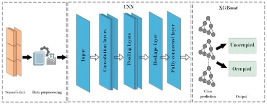
Figure 1.
Architecture of CNN-XGBoost model.
The first part of the model is a deep learning algorithm consisting of two key layers: the convolution layer which obtains the local features, and the pooling layer which performs a specific function such as max pooling, providing the maximum value in a filter region (see Figure 2).
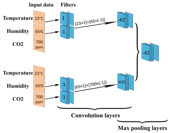
Figure 2.
An example of CNN architecture.
CNN part of the model receives the sensor data as input and learns the features of the data. This part has five layers: input, convolution, pooling, reshape, and fully connected layers. The input layer is a 3 × 1 vector that receives sensor data. First, we check the data for missing values and standardize them, and then the clean data are used as input of the CNN part of the model. An example of convolution and max pooling operations on indoor climate data is shown in Figure 2. The CNN part is trained by a backpropagation algorithm [45]. The XGBoost part of the model is a scalable end-to-end tree-boosting algorithm [43] that is replaced by the output layer of the CNN part [46]. To prevent overfitting, XGBoost uses the learning rate (or shrinkage) parameter and the number of trees parameter. The former manages the learning process by weighing new trees added to the model. The latter controls the number of trees.
XGBoost has outperformed other algorithms in many machine learning cases [47]. The XGBoost algorithm does not contain a feature learning part, and this problem can be solved by adding the convolution layer of a CNN to XGBoost [47]. The output of the XGBoost is either 0 or 1, where 0 stands for unoccupied and 1 stands for occupied.
2.2. Studied Rooms in a Residential Building
The developed model was validated using experimental data from three different rooms in a single-family house located on the northwestern outskirts of Copenhagen, Denmark. Figure 3 shows the building plan, in which the three rooms under study are highlighted. The details of the studied rooms are listed in Table 1. The rooms were mechanically ventilated with an air change rate of approximately 0.6 per hour during the experiment. All the windows and external doors were closed, whereas all the internal doors were open during the experiment. Even though the doors of the rooms were open during the test and the air was exchanged inside the house, in addition to the ventilation system, the proposed model could accurately detect presence and absence. These conditions indicate that we did not place any restrictions on the residents in this experiment, and the residents remained in normal living conditions.
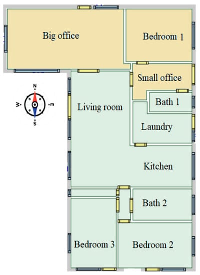
Figure 3.
The building’s floor plan.

Table 1.
Details of the rooms under study.
Two volunteers registered their presence for 13 days in December 2021 at 5 min time intervals. CO2 concentration, temperature, and relative humidity were measured and logged during this period with the same time interval. The sensors sent the climate data to cloud storage. To access the measured data, we use an application programming interface (API) through an open package provided for Python and Matlab programming languages.
2.3. Sensors
In this work, we used inexpensive sensors available in the market, i.e., CO2, temperature, and relative humidity sensors to facilitate the implementation of the method in any residential building. Simultaneously, we tried to use the fewest possible sensors. Although all sensors threaten privacy, we employed sensors that are commonly used in smart buildings today. The typical inaccuracy of the temperature and relative humidity sensors was ±0.2 °C and ±2% RH, respectively. The CO2 sensor was equipped with diffusion technology and intelligent calibration to measure the concentration of CO2 in the air. Table 2 depicts the specifications and the typical inaccuracies of the sensors.
Table 2.
Sensors’ specifications.
2.4. Data Collection
The total dataset contained 3612 records. We split the data into training and test datasets. Since our dataset was used for classification, the model was memoryless. Each set of inputs (CO2, temperature, and relative humidity) was mapped to a specific output (occupancy) independent of time. This feature enabled us to randomly select training and test datasets to increase the accuracy of the model. To compare the performance of the models, we used 20% of the data as test data [48]. The test data were not involved in the process of training. Thus, models were trained using only the training data. We used the same training and test datasets to train and test the available models. All hyperparameters of the classifiers were tuned before use. We performed an exhaustive search over large, specified parameters using a small portion of training data as a validation set, which was not presented for training. As shown in Figure 4, we were faced with an imbalanced occupancy dataset. To preserve the same proportion of occupancy and vacancy conditions in the test dataset, we used a stratified sampling method to sample test data from the original dataset.
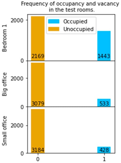
Figure 4.
The frequency of occupancy and vacancy in the studied rooms showing the presence of an imbalanced dataset.
To evaluate the power of the proposed method, we compared it with several machine learning algorithms: LR, DT, RF, GB, KMC, KNN, SV, CNN, and XGBoost classifiers. Considering the imbalanced data and binary classification, we used the F1 score (see Equation (3)) [49] to compare the methods. We also report the mean absolute error of each method.
F1 score is the harmonic mean of recall (Equation (1)) and precision (Equation (2)). Since the occupancy data were imbalanced, we used the F1 score instead of accuracy, because accuracy can be affected by a large number of zeros.
2.4.1. Bedroom 1
According to the plan of the building (see Figure 3), bedroom 1 had a window on the east wall. This window was closed during the experiment while the internal door to the small office was open during the experiment. Figure 5 shows the indoor climate data measured by the sensors and ground-truth data recorded by the occupants of bedroom 1. Figure 5 shows the existence of a pattern in CO2 time-series data associated with the presence and absence of occupants in this room, while we cannot see such an obvious pattern for temperature and relative humidity time-series data.
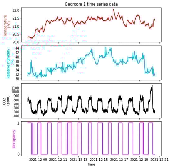
Figure 5.
Time-series plots of indoor climate and occupancy data measured for bedroom 1 from 8 December 2021 to 20 December 2022.
To better understand the relationship between the occupancy and indoor climate data in bedroom 1, the pairwise scatter plot is shown in Figure 6. On the diagonal of this matrix, we see the histogram of temperature, relative humidity, and CO2 distributions colored by occupancy and vacancy. For CO2, we can see two distinguishable distributions for occupied and unoccupied conditions. This did not happen for relative humidity and temperature. Both the mean and the median for CO2 data when the room was occupied were equal to 808. For unoccupied conditions, we had a mean and median equal to 534 and 525, respectively. It can be understood from the temperature–CO2 and humidity–CO2 plots that there were two separate clusters of data for occupancy and vacancy. In contrast, in the temperature–humidity plots, we could not easily separate occupancy from vacancy. These graphs indicate that the occupancy was mostly reflected in the CO2 measurements.
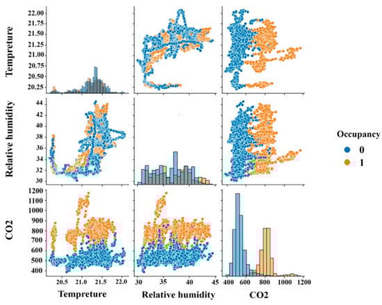
Figure 6.
Pairwise scatter plot of the indoor climate data for bedroom 1. Occupancy data are shown as a hue.
2.4.2. Small Office
There were four doors: the entrance door, the door to bedroom 1, the door to the living room, and the door to bath 1. The doors to bedroom 1 and the living room were always open during the experiment; hence, there was an air exchange between these rooms. Looking at the time-series data of this room (see Figure 7), we can see no obvious pattern in the CO2 and relative humidity plots associated with ground-truth occupancy data while the temperature plot shows a relatively cyclic pattern affiliated with occupancy. Later, we examined the effect of relative humidity and CO2 data on increasing the accuracy of occupancy prediction.
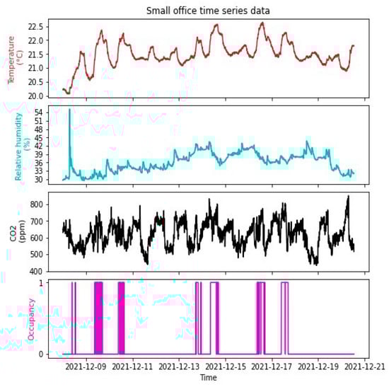
Figure 7.
Time-series plots of indoor climate and occupancy data measured for the small office from 8 December 2021 to 20 December 2022.
As displayed in Figure 8, there was no apparent linear correlation between indoor climate data. The mean temperature when the room was occupied was 22 °C. From the CO2–temperature plot, occupancy data were clumped at temperatures higher than 22 °C.
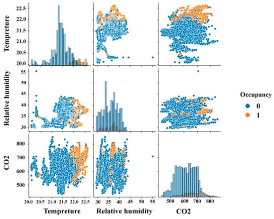
Figure 8.
Pairwise scatter plots of the indoor climate data for the small office. Occupancy data are shown as a hue.
2.4.3. Big Office
The big office had characteristics that caused the weakest occupancy prediction among all rooms under the study. This room was the largest in this study. This factor made it hard for sensors to accurately measure real-time changes in indoor climate. This room had two windows and two doors, one of which was always open to the living room during the study. This condition caused turbulence in the indoor climate.
This turbulence can be understood from the time-series plots (see Figure 9) of the big office indoor climate and occupancy data. Temperature and relative humidity showed no fluctuation affiliated with the occupancy data. The CO2 sensor showed a better performance compared to the other sensors, in measuring CO2 changes that arose from occupancy, although this performance was not as obvious as what we saw earlier for bedroom 1. Looking at Figure 10, we can see that occupancy was more connected to the CO2 data.
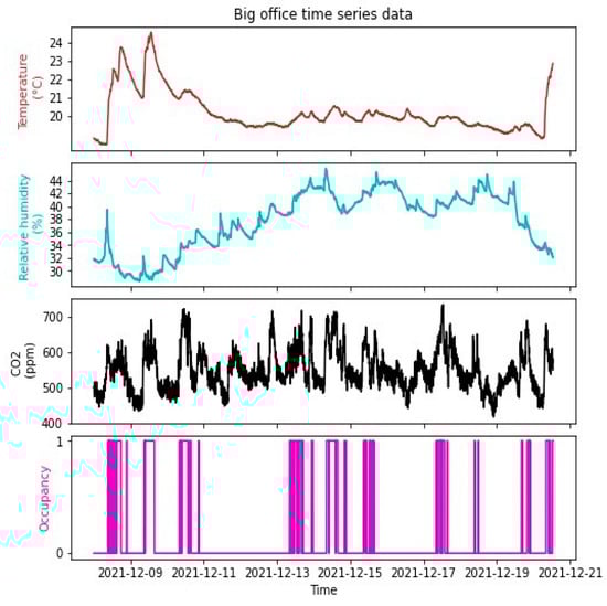
Figure 9.
Time-series plot of indoor climate and occupancy data measured for the big office from 8 December 2021 to 20 December 2022.
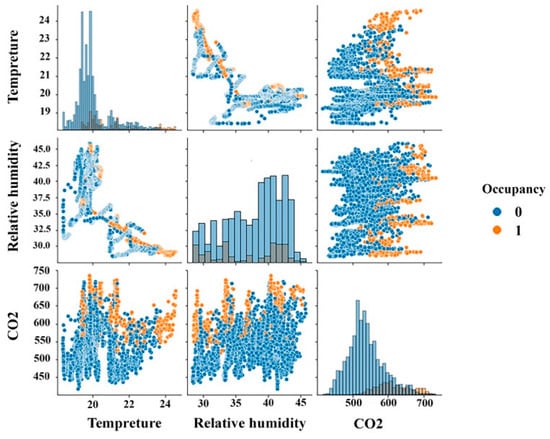
Figure 10.
Pairwise scatter plots of the indoor climate data for the big office. Occupancy data are shown as a hue.
3. Result and Discussion
This section aims to apply previously introduced machine learning models to the data collected from various rooms of the residential building explained in Section 2.4. We also compare the accuracy of the proposed model with other machine learning models using mean absolute error as a measure of prediction error. Considering the imbalanced data, we could not consider the ratio as a measure of accuracy. For example, in the small office, we had 428 ones against 3184 zeros. If a model can classify only zeros, then it can achieve high accuracy just by predicting zeros while it is unable to classify ones. We applied the F1 score as a measure of accuracy, whereby a model unable to classify ones would have a lower F1 score.
Below, model comparison tables are presented separately for the studied rooms. All hyperparameters of the classifiers were tuned before use. This process was performed using the GridSearchCV function in Python. We conducted an exhaustive search over large, specified parameters using this function. Table 3 shows the model comparison for bedroom 1. Our proposed classifier outperformed other classifiers with the highest F1 score equal to 0.986 and the lowest mean absolute error or misclassification rate [50] equal to 0.011.
Table 3.
Model comparison table for bedroom 1.
Some other classifiers performed similarly to our model, i.e., XGBoost and logistic regression. The reason was the strong correlation between occupancy and CO2 data in bedroom 1. If we look at the histogram of the CO2 data (see Figure 6), we can see that it followed a mixed distribution: one cluster of data with a mean equal to 534 when the room was unoccupied and another one with a mean equal to 808 when the room was occupied. This increased the power of the classifiers in predicting occupancy.
To check whether the other sensors, except CO2, improved the power of the classifier, we used only CO2 as input, and the result is depicted in Table 4.
Table 4.
CNN-XGBoost performance for bedroom 1 with CO2 as the only input.
The result shows that using only CO2 data significantly decreased the accuracy of the model. This means that the presence of the other sensors was vital to increasing the power of the classifier.
Table 5 shows the model comparison for the small office. In Table 5, we can see that SV was unable to predict vacancy. KNN and KMC showed poor performance in predicting occupancy. This was rooted in two issues: the imbalanced occupancy data and the inability of the indoor climate data to capture frequent changes between occupancy and vacancy. Here again, we can see that the proposed model showed the best performance among the other models. This means the purposed model could learn the relation between occupancy data and slight changes in indoor data. The misclassification rate was 0.029. This means that the model misclassified only 10 + 11 = 21 out of 722 occupied/unoccupied conditions.
Table 5.
Model comparison table for the small office.
As shown in Figure 8, there was a possible correlation between temperature and occupancy. The distribution of the temperature data in the small office showed no apparent signs of a mixed distribution; however, we examined whether eliminating CO2 and humidity worsened the prediction.
Table 6 shows that, by removing the CO2 and relative humidity data from the input, we obtained a worse prediction when predicting the occupancy of the small office.
Table 6.
CNN-XGBoost performance for the small office when the only input was temperature.
The final model comparison was performed for the big office. As shown earlier (see Figure 9 and Figure 10), there was no obvious pattern between the indoor climate data and occupancy data. Table 7 confirms this and shows that the classifiers were unable to predict occupancy accurately. As expected, the proposed model was convincingly the best model among those evaluated in this study. The misclassification ratio was 0.073. This ratio indicates that the model could predict 92.67% of occupied/unoccupied situations.
Table 7.
Model comparison table for the big office.
We increased the accuracy of the occupancy prediction in residential buildings with mechanical ventilation. This process was conducted by combining two leading methods to take advantage of the feature extraction capability of CNN with the speed, accuracy, and flexibility of XGBoost. We proposed an accurate model without using expensive privacy-invading camera-based implementations. The implementation of the model was performed simply by installing inexpensive sensors and connecting them to the classifier. The whole procedure is performed automatically from feature extracting to classification. This model can accurately predict the occupancy of residential buildings with a balanced mechanical ventilation system.
In three rooms, CNN-XGBoost showed that, even in the worst scenarios, it could precisely learn the relations between the input and the output data and consistently outperform the other available methods. In this work, we picked two methods (CNN and XGBoost) rarely used in building occupancy detection contexts [16,22] to examine the power of these models separately and combined. Despite XGBoost, which showed the best performance after CNN-XGBoost in two of three rooms, CNN worked poorly in the small and big offices. The performance of XGBoost confirmed that XGBoost needs a feature learning part, which can be solved by adding the convolution layer of a CNN to XGBoost [47].
In the end, it is good to briefly state some limitations of this research. To collect the most accurate ground-truth data, we asked the occupants to register their presence in a 5 min time interval, rather than using other occupancy sensors. Therefore, this limited the period of collecting ground-truth data to 13 days. The period was only in winter when the windows are usually closed. In future work, the proposed model should be validated for an extended period and in different seasons. More diverse data can increase the accuracy of the model. Furthermore, during the experiment, the ventilation rate was constant. It is recommended to test the model in buildings with variable air volume ventilation systems.
4. Conclusions and Recommendations for Future Research
In this paper, we proposed a CNN-XGBoost model for occupancy detection in residential buildings with a balanced mechanical ventilation system using indoor climate sensors. Unlike previous studies that applied complex implementation to both models and sensors, our method uses a simple deep learning model and inexpensive sensors. Instead of using a test room and placing some restrictions, we validated our model in a single-family residential building and did not impose any restrictions on the use of doors, windows, HVAC, etc.
The presented model consists of a CNN part that automatically extracts features of indoor climate data and a XGBoost part that is a scalable gradient-boosted decision tree ML algorithm. We compared our proposed model with a range of occupancy detection models. Our proposed model outperformed all other approaches. In two of three study rooms, XGBoost had the best performance after CNN-XGBoost. Ignoring the execution time of the two methods due to their nature, i.e., gradient boosting and neural network, the difference between the MAEs was less than 0.01. Although this difference may seem low, it caused more than a 15% difference in false predictions (FP + FN). This difference indicates the importance of the CNN part. Although relative humidity and temperature measurements have little effect on occupancy detection, the proposed model can learn the relationship between minor changes in humidity and temperature and occupancy. The big office was the largest room with the weakest results for occupancy detection. Due to the dimensions of the big office, finding the optimal place to install the sensor would improve the results.
For future research, the model can be applied to the measurements of the sensors installed in several locations and heights. The best place for installing the sensor would be that with the best results. Another solution to this issue is to use more than one sensor in the big office and compare the result with the current situation. We used our model in a building with a mechanical ventilation system. Using the proposed model in buildings with natural ventilation systems is recommended. Lastly, the proposed model can be implemented to detect not only presence and absence, but also the number of occupants in residential buildings.
Author Contributions
Supervision, S.R. and A.A.; Writing—original draft, A.M. All authors have read and agreed to the published version of the manuscript.
Funding
This research work was conducted as part of a project called SmartVENT. The Energy Technology Development and Demonstration Program (EUDP) financially supported this work (Journal No. 64018-0501).
Institutional Review Board Statement
Not applicable.
Informed Consent Statement
Not applicable.
Data Availability Statement
The datasets involved in the current study are available from the corresponding author, A.M. (abolfazlms13@gmail.com) upon reasonable request.
Conflicts of Interest
The authors declare no conflict of interest.
Nomenclature
| LR | Logistic regression |
| DT | Decision tree |
| RF | Random forest |
| GB | Gradient boosting |
| KMC | K-means clustering |
| KNN | K-nearest neighbors |
| SV | Support vector |
| CNN | Convolutional neural network |
| XGBoost | Extreme gradient boosting |
| CNN-XGBoost | Convolutional neural network extreme gradient boosting |
| TP | True positive: number of conditions correctly identified as unoccupied |
| TN | True negative: number of conditions correctly identified as occupied |
| FP | False positive: number of conditions incorrectly identified as unoccupied |
| FN | False negative: number of conditions incorrectly identified as occupied |
| ppm | Parts per million |
| RH | Relative humidity |
| p | Probability |
| MAE | Mean absolute error |
References
- Final Energy Consumption by Sector, EU. 2020. Available online: https://ec.europa.eu/eurostat/statistics-explained/index.php?title=Energy_statistics_-_an_overview#Final_energy_consumption (accessed on 10 January 2021).
- Final Energy Consumption in the Residential Sector by Use, EU. 2020. Available online: https://ec.europa.eu/eurostat/statistics-explained/index.php?title=File:Final_energy_consumption_in_the_residential_sector_by_use,_EU,_2020_v5.png (accessed on 10 January 2021).
- Delzendeh, E.; Wu, S.; Lee, A.; Zhou, Y. The impact of occupants’ behaviours on building energy analysis: A research review. Renew. Sustain. Energy Rev. 2017, 80, 1061–1071. [Google Scholar] [CrossRef]
- He, Z.; Hong, T.; Chou, S.K. A framework for estimating the energy-saving potential of occupant behaviour improvement. Appl. Energy 2021, 287, 116591. [Google Scholar] [CrossRef]
- Pan, S.; Wang, X.; Wei, S.; Xu, C.; Zhang, X.; Xie, J.; Tindall, J.; de Wilde, P. Energy waste in buildings due to occupant behaviour. Energy Procedia 2017, 105, 2233–2238. [Google Scholar] [CrossRef]
- Candanedo, L.M.; Feldheim, V. Accurate occupancy detection of an office room from light, temperature, humidity and CO2 measurements using statistical learning models. Energy Build. 2016, 112, 28–39. [Google Scholar] [CrossRef]
- Yang, Z.; Becerik-Gerber, B. How does building occupancy influence energy efficiency of HVAC systems? Energy Procedia 2016, 88, 775–780. [Google Scholar] [CrossRef]
- Yang, Z.; Becerik-Gerber, B. Modeling personalized occupancy profiles for representing long term patterns by using ambient context. Build. Environ. 2014, 78, 23–35. [Google Scholar] [CrossRef]
- Kwok, S.S.; Yuen, R.K.; Lee, E.W. An intelligent approach to assessing the effect of building occupancy on building cooling load prediction. Build. Environ. 2011, 46, 1681–1690. [Google Scholar] [CrossRef]
- da Silva, P.C.; Leal, V.; Andersen, M. Occupants interaction with electric lighting and shading systems in real single-occupied offices: Results from a monitoring campaign. Build. Environ. 2013, 64, 152–168. [Google Scholar] [CrossRef]
- Labeodan, T.; De Bakker, C.; Rosemann, A.; Zeiler, W. On the application of wireless sensors and actuators network in existing buildings for occupancy detection and occupancy-driven lighting control. Energy Build. 2016, 127, 75–83. [Google Scholar] [CrossRef]
- Peruffo, A.; Pandharipande, A.; Caicedo, D.; Schenato, L. Lighting control with distributed wireless sensing and actuation for daylight and occupancy adaptation. Energy Build. 2015, 97, 13–20. [Google Scholar] [CrossRef]
- Agarwal, Y.; Balaji, B.; Dutta, S.; Gupta, R.K.; Weng, T. Duty-cycling buildings aggressively: The next frontier in HVAC control. In Proceedings of the 10th ACM/IEEE International Conference on Information Processing in Sensor Networks, Chicago, IL, USA, 12–14 April 2011; pp. 246–257. [Google Scholar]
- Wang, F.; Feng, Q.; Chen, Z.; Zhao, Q.; Cheng, Z.; Zou, J.; Zhang, Y.; Mai, J.; Li, Y.; Reeve, H. Predictive control of indoor environment using occupant number detected by video data and CO2 concentration. Energy Build. 2017, 145, 155–162. [Google Scholar] [CrossRef]
- Purdon, S.; Kusy, B.; Jurdak, R.; Challen, G. Model-free HVAC control using occupant feedback. In Proceedings of the 38th Annual IEEE Conference on Local Computer Networks-Workshops, Sydney, Australia, 21–24 October 2013; pp. 84–92. [Google Scholar]
- Jin, Y.; Yan, D.; Chong, A.; Dong, B.; An, J. Building occupancy forecasting: A systematical and critical review. Energy Build. 2021, 251, 111345. [Google Scholar] [CrossRef]
- Salimi, S.; Liu, Z.; Hammad, A. Occupancy prediction model for open-plan offices using real-time location system and inhomogeneous Markov chain. Build. Environ. 2019, 152, 1–6. [Google Scholar] [CrossRef]
- Erickson, V.L.; Carreira-Perpiñán, M.Á.; Cerpa, A.E. OBSERVE: Occupancy-based system for efficient reduction of HVAC energy. In Proceedings of the 10th ACM/IEEE International Conference on Information Processing in Sensor Networks, Chicago, IL, USA, 12–14 April 2011; pp. 258–269. [Google Scholar]
- Li, Z.; Dong, B. Short term predictions of occupancy in commercial buildings—Performance analysis for stochastic models and machine learning approaches. Energy Build. 2018, 158, 268–281. [Google Scholar] [CrossRef]
- Huang, W.; Lin, Y.; Lin, B.; Zhao, L. Modeling and predicting the occupancy in a China hub airport terminal using Wi-Fi data. Energy Build. 2019, 203, 109439. [Google Scholar] [CrossRef]
- Pedersen, T.H.; Nielsen, K.U.; Petersen, S. Method for room occupancy detection based on trajectory of indoor climate sensor data. Build. Environ. 2017, 115, 147–156. [Google Scholar] [CrossRef]
- Dai, X.; Liu, J.; Zhang, X. A review of studies applying machine learning models to predict occupancy and window-opening behaviours in smart buildings. Energy Build. 2020, 223, 110159. [Google Scholar] [CrossRef]
- Killian, M.; Kozek, M. Short-term occupancy prediction and occupancy based constraints for MPC of smart homes. IFAC-PapersOnLine 2019, 52, 377–382. [Google Scholar] [CrossRef]
- Chatterjee, A. An introduction to the proper orthogonal decomposition. Curr. Sci. 2000, 10, 808–817. [Google Scholar]
- Li, N.; Calis, G.; Becerik-Gerber, B. Measuring and monitoring occupancy with an RFID based system for demand-driven HVAC operations. Autom. Constr. 2012, 24, 89–99. [Google Scholar] [CrossRef]
- Peng, Y.; Rysanek, A.; Nagy, Z.; Schlüter, A. Using machine learning techniques for occupancy-prediction-based cooling control in office buildings. Appl. Energy 2018, 211, 1343–1358. [Google Scholar] [CrossRef]
- Aftab, M.; Chen, C.; Chau, C.K.; Rahwan, T. Automatic HVAC control with real-time occupancy recognition and simulation-guided model predictive control in low-cost embedded system. Energy Build. 2017, 154, 141–156. [Google Scholar] [CrossRef]
- Razavi, R.; Gharipour, A.; Fleury, M.; Akpan, I.J. Occupancy detection of residential buildings using smart meter data: A large-scale study. Energy Build. 2019, 183, 195–208. [Google Scholar] [CrossRef]
- Mamidi, S.K.; Chang, Y.H.; Maheswaran, R. Adaptive Learning Agents for Sustainable Building Energy Management. In 2012 Accociation for the Advanced of Artificial Intelligence (AAAI) Spring Symposium Series; Association for the Advancement of Artificial Intelligence (AAAI): Los Angeles, CA, USA, 2012. [Google Scholar]
- Sangogboye, F.C.; Arendt, K.; Singh, A.; Veje, C.T.; Kjærgaard, M.B.; Jørgensen, B.N. Performance comparison of occupancy count estimation and prediction with common versus dedicated sensors for building model predictive control. In Building Simulation; Tsinghua University Press: Beijing, China, 2017; Volume 10, pp. 829–843. [Google Scholar]
- Kampezidou, S.I.; Ray, A.T.; Duncan, S.; Balchanos, M.G.; Mavris, D.N. Real-time occupancy detection with physics-informed pattern-recognition machines based on limited CO2 and temperature sensors. Energy Build. 2021, 242, 110863. [Google Scholar] [CrossRef]
- Kim, S.; Kang, S.; Ryu, K.R.; Song, G. Real-time occupancy prediction in a large exhibition hall using deep learning approach. Energy Build. 2019, 199, 216–222. [Google Scholar] [CrossRef]
- Leeraksakiat, P.; Pora, W. Occupancy forecasting using lstm neural network and transfer learning. In Proceedings of the 2020 17th International Conference on Electrical Engineering/Electronics, Computer, Telecommunications and Information Technology (ECTI-CON), Virtual, 24–27 June 2020; pp. 470–473. [Google Scholar]
- Sama, S.K.; Rahnamay-Naeini, M. A study on compression-based sequential prediction methods for occupancy prediction in smart homes. In Proceedings of the 2016 IEEE 7th Annual Ubiquitous Computing, Electronics & Mobile Communication Conference (UEMCON), New York, NY, USA, 20–22 October 2016; pp. 1–8. [Google Scholar]
- Liang, X.; Hong, T.; Shen, G.Q. Occupancy data analytics and prediction: A case study. Build. Environ. 2016, 102, 179–192. [Google Scholar] [CrossRef]
- Nacer, A.; Marhic, B.; Delahoche, L.; Masson, J.B. ALOS: Automatic learning of an occupancy schedule based on a new prediction model for a smart heating management system. Build. Environ. 2018, 142, 484–501. [Google Scholar] [CrossRef]
- Ding, Y.; Han, S.; Tian, Z.; Yao, J.; Chen, W.; Zhang, Q. Review on occupancy detection and prediction in building simulation. In Building Simulation; Tsinghua University Press: Beijing, China, 2021; pp. 1–24. [Google Scholar]
- Chen, Z.; Jiang, C.; Xie, L. Building occupancy estimation and detection: A review. Energy Build. 2018, 169, 260–270. [Google Scholar] [CrossRef]
- Trivedi, D.; Badarla, V. Occupancy detection systems for indoor environments: A survey of approaches and methods. Indoor Built Environ. 2020, 29, 1053–1069. [Google Scholar] [CrossRef]
- Zhang, W.; Wu, Y.; Calautit, J.K. A review on occupancy prediction through machine learning for enhancing energy efficiency, air quality and thermal comfort in the built environment. Renew. Sustain. Energy Rev. 2022, 167, 112704. [Google Scholar] [CrossRef]
- Sayed, A.N.; Himeur, Y.; Bensaali, F. Deep and transfer learning for building occupancy detection: A review and comparative analysis. Eng. Appl. Artif. Intell. 2022, 115, 105254. [Google Scholar] [CrossRef]
- Candanedo, L.M.; Feldheim, V.; Deramaix, D. A methodology based on Hidden Markov Models for occupancy detection and a case study in a low energy residential building. Energy Build. 2017, 148, 327–341. [Google Scholar] [CrossRef]
- Chen, T.; Guestrin, C. Xgboost: A scalable tree boosting system. In Proceedings of the 22nd Acm Sigkdd International Conference on Knowledge Discovery and Data Mining, San Francisco, CA, USA, 13–17 August 2016; pp. 785–794. [Google Scholar]
- LeCun, Y.; Boser, B.; Denker, J.; Henderson, D.; Howard, R.; Hubbard, W.; Jackel, L. Handwritten digit recognition with a back-propagation network. Adv. Neural Inf. Processing Syst. 1989, 2, 41–46. [Google Scholar]
- Chauvin, Y.; Rumelhart, D.E. Backpropagation: Theory, Architectures, and Applications; Taylor & Francis Group, Taylor & Francis Group: Los Angeles, CA, USA, 2013. [Google Scholar]
- Ren, X.; Guo, H.; Li, S.; Wang, S.; Li, J. A novel image classification method with CNN-XGBoost model. In International Workshop on Digital Watermarking; Springer: Cham, Switzerland, 2017; pp. 378–390. [Google Scholar]
- Thongsuwan, S.; Jaiyen, S.; Padcharoen, A.; Agarwal, P. ConvXGB: A new deep learning model for classification problems based on CNN and XGBoost. Nucl. Eng. Technol. 2021, 53, 522–531. [Google Scholar] [CrossRef]
- Gholamy, A.; Kreinovich, V.; Kosheleva, O. Why 70/30 or 80/20 Relation between Training and Testing Sets: A Pedagogical Explanation; Departmental Technical Reports (CS). 1209; University of Texas at El Paso: El Paso, TX, USA, 2018; Available online: https://scholarworks.utep.edu/cs_techrep/1209 (accessed on 10 January 2021).
- Chinchor, N.; Sundheim, B.M. MUC-5 evaluation metrics. In Proceedings of the Fifth Message Understanding Conference (MUC-5), Baltimore, Maryland, 25–27 August 1993. [Google Scholar]
- Dey, N.; Borah, S.; Babo, R.; Ashour, A.S. Social Network Analytics: Computational Research Methods and Techniques; Academic Press: Cambridge, MA, USA, 2018. [Google Scholar]


Publisher’s Note: MDPI stays neutral with regard to jurisdictional claims in published maps and institutional affiliations. |
© 2022 by the authors. Licensee MDPI, Basel, Switzerland. This article is an open access article distributed under the terms and conditions of the Creative Commons Attribution (CC BY) license (https://creativecommons.org/licenses/by/4.0/).