Abstract
The appropriate feature/predictor selection is as significant as building efficient estimation methods for the accurate estimation of power consumption, which is required for self-awareness and autonomous decision systems. Traditional methodologies define predictors by assessing whether there is a relationship between the predictors and the response variable. Contrarily, this study determines predictors based on their individual and group impacts on the estimation accuracy directly. To analyze the impact of predictors on the power-consumption estimation of an IT rack in a data center, estimations were carried out employing each prospective predictor separately using the measured data under the real-world workload. Then, the ratio of CPU usage was set as the default predictor, and the remaining variables were assigned as the second predictor one by one. By utilizing the same approach, the best combination of predictors was determined. As a result, it was discovered that some variables with a low correlation coefficient with power consumption improved the estimation accuracy, whereas some variables with high correlation coefficients worsened the estimation result. The CPU is the most power-consuming component in the server and one of the most used predictors in the literature. However, the estimation accuracy obtained using only the CPU is 10 times worse than the estimation result conducted by utilizing the predictor set determined at the end of the experiments. This study shows that instead of choosing predictors only from one point of view or one method, it is more convenient to select predictors by assessing their influence on estimation results. Examining the trend and characteristics of the estimated variable should also be considered.
1. Introduction
1.1. Background and Motivation
In recent years, the number of Internet of Things (IoT)-connected devices and smart and autonomous systems, as well as the volume of data generated, has dramatically increased [1,2]. The storage and processing of real digital data are much more advanced, significant, and simple today. Moreover, the diversity, accessibility, and reliability of the measured data have increased compared to the past. Consequently, the efficiency of various applications for the decision-making process has improved. This development has become very useful, especially for smart-grid applications in terms of providing the ability to manage demand and generation through demand side management (DSM). One of the most important issues for DSM and power systems is to forecast electrical power consumption in order to balance generation and demand, as well as the efficient planning, operation, and management of electric power systems [3,4]. Accurate estimation results are critical for both consumers and utilities in order to prevent additional operating costs, energy waste, unnecessary energy purchases, and energy reserves [5]. However, obtaining accurate load-forecasting results is still a challenging task, as it is influenced by consumption patterns, environmental and socio-economic parameters, and weather conditions [6]. Therefore, in order to obtain accurate and reliable forecasting results, it is crucial to choose the most appropriate combination of predictors, also known as independent variables, that affect the forecasted variable [7]. In terms of energy and thermal management, accurate estimation of power consumption is also significant for data centers [8], which are important players in DSM due to their huge and flexible load characteristics. In the literature, many studies related to DC’s participation in DSM [9,10,11,12], power consumption, and forecasting models for subcomponents of DCs have been carried out [3,7,13,14,15,16]. According to [17], the most power-consuming part of a typical data center is servers, with a ratio of 56%, followed by cooling devices, with a ratio of 30%. The power-conditioning infrastructures are responsible for consuming 8% of the total power consumption in a DC, whereas the network equipment and lighting are responsible for 5% and 1%, respectively. The largest proportion of power consumption is consumed by servers, and this also affects the power consumption of cooling equipment.
The main motivation of this study is to examine the impact of predictors on power-consumption estimation of an IT rack that contains servers. One of the main problems for power forecasting is the predictor-selection process, especially for data centers, because too many features might be obtained from a huge amount of measured data. Moreover, the execution time and accuracy of the estimation also depend on predictors, which are crucial for a power-consumption model.
However, in order to determine the most convenient predictors, recent studies generally prefer to utilize only correlation analysis or another specific feature-selection method, instead of taking into account the direct effect of predictors on estimation results [4,6,7,18,19,20,21,22,23,24]. In this paper, the individual and group effects of various variables (e.g., CPU and RAM usage ratios, temperature, network load, etc.) on power consumption estimation have been investigated using actual data measured from IoT-based sensors, energy analyzers, and an IT rack in a data center. The power consumption of the IT rack is initially forecasted using each variable/predictor individually and the estimation result is examined. Then, each variable in turn is used as a second predictor in addition to the CPU usage ratio, which is determined as the first predictor since it is the most commonly used variable for power-consumption models of servers in the literature [8,25,26,27]. Finally, the best combination of predictors is determined using a similar approach and a trial-and-error method. The estimation results are examined using various error metrics and data trends & characteristics.
1.2. Literature Review
According to recent studies, server power-consumption models for estimation, power management, and load balancing [8] generally depend on CPU utilization. Yao et al. [25] proposed a power-consumption model for each server that has a linear relationship between CPU utilization and frequency. Another study [26] modelled the energy consumption of the server as the sum of individual energy consumption of CPU and memory. Berezovskaya et al. [28] proposed a toolbox for building a modular model of a data center using a linear power-consumption model for IT equipment that takes into account the CPU utilization, CPU temperature, and power consumption of the server’s fan. Daraghmeh et al. [27] also used a linear power-consumption model as a function of CPU utilization to calculate the power consumption of servers using a synthetic test workload. As stated in [8], although CPU utilization is the most used variable for building the power-consumption model of a server, CPU frequency, temperature, and memory utilization come next. On the other hand, the CPU is responsible for merely about 32% of the total power consumption of the server; the remaining amount is caused by other subcomponents [8,29]. Thus, the variables only dependent on the CPU are not sufficient to build an accurate power-consumption model for servers since other variables can directly or indirectly affect power consumption. In a review paper focusing on the energy efficiency of small and medium data centers [13], various strategies and power-consumption models, including parameters such as the CPU, memory, hard disk, network interface card, uninterruptible power supply (UPS), have been examined [14]. In [15], the server’s power consumption is forecasted using artificial neural network-based models using the variables CPU, memory, and disk under different workload types. While proposing power consumption equations of servers for forecasting models, some studies focused on power-consuming components of servers such as memory, disk, network interface card, fan, and especially CPU [13,14,15]. However, even though the total power consumption of the server is the sum of the individual power consumptions of these parameters, there may be other factors that affect the total power consumption, such as room and outside temperatures, humidity, timestamp, network load, etc. Thus, selecting the right parameters that affect the server’s power consumption is critical for accurate power-consumption estimation. To this end, many studies have used different feature-selection methods and determined the most suitable combination of predictors for estimation [4,6,7,14,18,19,20]. The studies related to feature-selection methods are summarized in Table 1.

Table 1.
Studies related to feature-selection methods.
1.3. Contributions
As seen in the compact literature review above, although the experiments in many studies were conducted using a real PC or server, they were carried out for dummy test environments created with synthetic workloads where different scenarios were tried. Moreover, conventional approaches for determining predictors are generally based on examining whether there is a correlation between the predictors and the response variable by using various metrics, and the predictors are determined at once according to the results of these metrics. The authors mostly focused on the effect of feature sets created by comparing various feature-selection methods on the improvement of estimation accuracy. However, experimental research from the perspective of examining the individual and group effects of predictors on the forecasting accuracy directly, and determining the predictors according to this analysis, is still lacking.
This study is intended to fill in this gap and provides an approach for determining the most suitable predictors to forecast the power consumption of an IT rack. The main contributions of this paper are summarized as follows:
- The analyses and experiments were performed by measuring and processing the actual sensor data from a data center, as well as using actual data from an IT rack operating under routine real workloads and circumstances for the period between April 2020 and February 2021.
- While determining the predictors, not only a single error metric but also seven different metrics were taken into account for comparing the estimation accuracy.
- Instead of determining the predictors based on the relationship of the variables with each other using any metric, the predictors were determined by examining their direct effects on estimation results via various experiments.
- The individual and group effects of predictors on estimation accuracy were examined in detail.
- Contrary to the assumption that a variable with a high correlation coefficient affects estimation accuracy better as in many studies, it was discovered that some variables increase the error rate of the estimation even if their correlation coefficients are high, whereas some variables reduce the error rate despite having low correlation coefficients.
- It was concluded that another set of variables in addition to the CPU-related variables is required when estimating IT power consumption.
- It was established that simply looking at the correlation matrix or directly selecting the predictors that cause the lowest estimation-error rate is not the best way to determine predictors. The trend and characteristics of the estimated variable are also significant in terms of determining predictors. Furthermore, trial-and-error methods should also be used by trying several combinations of predictors.
The remainder of this paper is organized as follows. Section 2 describes the methodology, experimental environment, and main components of performance analysis. The content of experiments for exploring predictors’ effects on power-consumption estimation for an IT rack is also explained in Section 2. The results and discussion are presented in Section 3. Finally, conclusions are given in Section 4.
2. Experimental Environment
Firstly, the methodology adopted in this study is described in Section 2. Secondly, the experiment layout is explained, and then the process of the correlation analysis and the structure of the estimation algorithm for the power consumption of an IT rack are explained. After that, the definitions of error metrics used for comparing the performance of experiments are given. Finally, the details of the experiments are explained.
2.1. Methodology
The general flowchart of the methodology, which was composed of three research steps, is shown in Figure 1. In the first step, the data pre-processing was performed for the defined time horizon, which was between April 2020 and February 2021. This step started with converting the raw data received in JSON format to CSV format with a script written in MATLAB. Then, the process continued by filling in missing data, detecting outliers, smoothing data, and synchronizing all data that had different resolutions into 60 min intervals. The data synchronizing was carried out with the “synchronize” function that concatenated the data, including various variables, horizontally and then resampled or aggregated the data using linear interpolation. The “filloutliers” function determined the data that were more than three standard deviations from the mean as outliers and filled them with the nearest non-outlier values. The “smoothdata” function smoothed the data by taking the moving average over a 3 h window. Thereafter, all data were separated into categories based on the devices and sensors to which they belonged. After that, 70 different variables/features were determined, including the airflow temperatures of eight air conditioners in the data center, row-flow temperatures in three different locations, indoor temperatures and humidity in six different locations, front and rear temperatures of the ARGE rack, the power consumption of each server in the ARGE rack, time-related parameters, and IT parameters such as network-traffic load and the ratio of CPU and RAM usage.
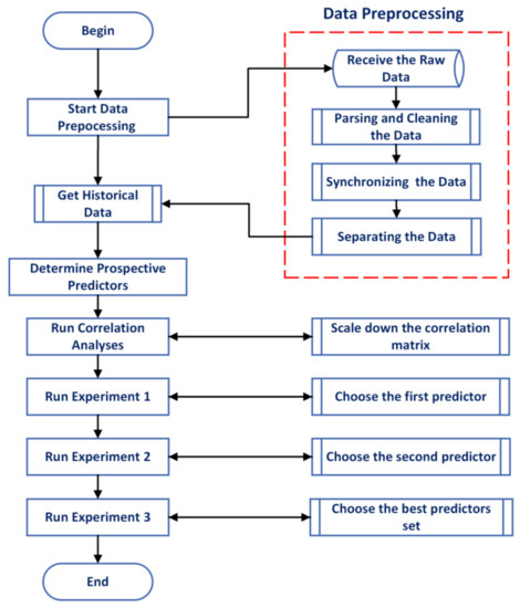
Figure 1.
General flowchart of the methodology.
In the second step, the correlation matrix was created for 70 variables, and then it was shrunk by removing variables that had poor correlations with the power consumption of the ARGE rack. The details of the correlation analysis explained in Section 2.3.
In the third step, the individual and group effects of predictors on estimation results were examined through experiments 1–2 and 3, and the most appropriate predictors were determined as a result. The details of the experiments are explained in Section 2.6.
2.2. Experimental Layout
In this study, all analyses were performed using data from a data center called the GreenDC within the scope of the project “Sustainable energy demand side management for GREEN Data Centers,” which was funded by the EU Horizon MSCA. The data were measured between April 2020 and February 2021. The data-collection model consisted of two parts related to infrastructure and IT. Data-center infrastructure-management software DCIM was used to log the whole infrastructure part. The physical infrastructure consisted of UPS, generators, chillers, air conditioners, and IT racks. In the GreenDC, one rack cabinet called the ARGE rack was used for the experiments. The ARGE rack contains 10 servers, five of which have an Intel® Xeon® E5-2630 v3 processor, ECC DDR4 300 GB RAM, and a 40 TB hard disk, and the other five of which have an Intel® Xeon® E7-4830 v3 processor, ECC DDR4 500 GB RAM, and a 240 GB hard disk. The power consumption of the servers in the ARGE rack is measured by smart PDUs [43]. Furthermore, energy analyzers were installed at the electrical panel in the GreenDC and each air conditioner and chiller in order to measure the power consumption of the whole DC, air conditioner, and chiller individually. Furthermore, various IoT-based sensors were installed at different locations in the GreenDC to measure the inside temperature and humidity, airflow temperatures of each air conditioner, temperatures of the row flows, and the ambient temperature outside. Moreover, three sensors were mounted on the front door of the ARGE rack and three on the back door to track temperature changes between the inlet and outlet of the rack. The data associated with IT were also measured via Zabbix, which is an IT management/monitoring software. All data were measured under the real-world workload instead of using a dummy workload. After the data-collection phase, all data were stored in JSON format.
2.3. Correlation Analysis
Correlation analysis is frequently utilized to evaluate the relationship between variables and determine the suitable ones as predictors to be used in estimation algorithms [18,21,22,23,24]. Thus, in this study, the correlation matrix, which includes Pearson correlation coefficients, was initially created for 70 variables obtained from measured data in order to determine prospective predictors and reveal their effects on the power consumption of the ARGE rack. Additionally, the effectiveness of employing correlation analysis to choose predictors was explored. The initial correlation matrix was scaled down by discarding variables whose correlation coefficients with the power consumption of the ARGE rack were between −0.2 and +0.2. The new correlation matrix, which demonstrates the relationship between the most suitable variables, is shown in Figure 2. Additionally, the probable predictors are given in Table 2. The response variable TotalPowerCons represents the total power consumption of 10 servers in the ARGE rack.
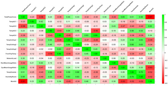
Figure 2.
Correlation matrix.
Table 2.
Probable predictors for estimation of IT power consumption.
The airflow temperatures of the air conditioners, which were placed in different locations in the GreenDC, are indicated by TempAC. The data center’s indoor temperatures, which were measured by IoT-based sensors mounted in various locations on the ceiling of the GreenDC, are denoted by TempCeiling. FrontTopTemp represents the top of the front door’s temperature of the ARGE rack. The total in/out network traffic load is indicated by NetworkLoad. The mean of 10 servers’ CPU- and RAM-usage ratios in the ARGE rack are represented by CpuMeanUsageRatio and RamMeanUsageRatio, respectively. Mean outside temperature is denoted by TempOutside, whereas mean room humidity is represented by HumidityRoom.
In order to reveal the actual and full effects of time parameters, we separated the time parameters as sine and cosine parts of it because time has a cyclic characteristic. For example, if the months in a year are considered just numbers in a straight line, it can be said that the number 7 is closer to 12 than the number 2. However, the second month is closer to the twelfth month than the seventh month in the cycle of time. Thus, sine and cosine parts of month data were calculated as shown in Equations (1) and (2) and are represented by MonthX and MonthY, respectively.
MonthNumber indicates the order of the month in a year to which the measured data belong (e.g., 5 means May).
2.4. Estimation Algorithm for Power Consumption of the ARGE Rack
The scope of this study is to analyze the impact of each possible predictor on the estimation accuracy, rather than focusing on the accuracy of estimation methods. Thus, only a nonlinear regression model was used for power consumption estimation of the ARGE rack to evaluate the influences of the predictors. A nonlinear function of predictors was used in the calculation of the response variable by utilizing the nonlinear regression method, whose general mathematical form is represented in Equation (3).
is the observation of the response variable y, whereas denotes the observation of the predictor . The coefficient vector is represented by and the random error is indicated as . The relationship function between and is nonlinear. In this study, a nonlinear power-consumption model, which is shown in Equation (4), was utilized to estimate the power consumption of the ARGE rack.
The observation number is represented by i; coefficients of the equation are indicated by a, b, and c; and the number of independent variables (predictors) is shown as m. In the estimation process, historical data were required for both the dependent (response) and independent variables (predictors). The response variable is the power consumption of the ARGE rack. Probable predictors, which are listed in Table 2, are indicated as ,. In the estimation process, 80% of the historical data was used for training, whereas 20% was used for testing. Therefore, the historical data from 1 April through 23 December 2020 were used for training, whereas the data between 24 December 2020 to 28 February 2021 were used for testing. The nlinfit function under the statistics and machine-learning toolbox in MATLAB was used for the calculations.
2.5. Performance Evaluation Metrics
Despite the fact that there are several types of metrics for evaluating the performance of estimation results, there is no consensus among academics as to which one is the most effective because each one has its pros and cons [44]. In addition, the effectiveness and usefulness of various error metrics range depending on the different situations and the characteristics of the data set [45]. For example, the metrics mean square error (MSE), mean absolute error (MAE), and RMSE are scale-dependent measures, whereas the root mean square percentage error (RMSPE), symmetric mean absolute percentage error (sMAPE), and MAPE are based on percentage errors. Additionally, Koehler and Hyndman proposed a metric, the mean absolute scaled error (MASE), that is independent of the scale of the data and allows for effective comparison between different estimation models [45]. These error metrics can be mathematically calculated by Equations (6)–(12) below. The calculation of estimation error is shown in Equation (5), where represents the measured value at time and represents the estimated value of at time .
Let denote the forecast horizon, represents the mean operation, and indicates the observation number.
Although MAPE is commonly used to evaluate the accuracy of estimation models because it is easier to interpret, RMSE is also used to a considerable extent in terms of its theoretical importance in statistical models [45]. In this study, even though the estimation results were primarily compared using MAPE, other metrics were also calculated for each estimation result and all metrics were given together to analyze the changes in detail.
2.6. Experiments
Generally, variables that have higher correlation coefficients with the response variable are used as predictors because they are assumed to affect estimation results more than other variables without analyzing how those variables affect the estimation result individually or as a whole. Along with the experiments, the accuracy of this idea was investigated. According to the literature, the power consumption of servers is generally formulated based on the functions of CPU usage; thus, the impact of the CPU-usage ratio on the estimation of IT power consumption was primarily examined, and then the effects of all other variables were explored. For this purpose, three experiments are conducted and explained below.
2.6.1. Experiment 1: The Individual Effect of Predictors
Due to the fact that determining the most appropriate predictors is as significant as developing a suitable estimation model to achieve efficient and accurate estimation results, the effect of each predictor on estimation accuracy was investigated in this experiment. The variables listed in Table 2 were utilized individually as a predictor in the estimation model defined in Equation (4), and then the power consumption of the ARGE rack was estimated. The error rates of the estimation results, which were obtained using one variable from Table 2 as a predictor, are given in Table 3. Graphs of the estimation results are depicted in Figure 3. Among the prospective predictors, the impact of the variable CpuMeanUsageRatio was mainly investigated since it has been used in the literature as the most important parameter in modelling the power consumption of servers.
Table 3.
Error metrics for the estimation conducted using each predictor individually.
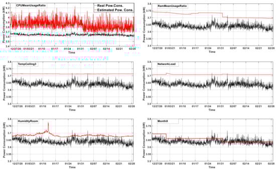
Figure 3.
The results of power consumption estimation of the ARGE rack that are performed using each predictor individually.
2.6.2. Experiment 2: Group Effects of Predictors
Since CPU is one of the most important parameters, it was set as the default predictor in the power-consumption model defined in Equation (4). Then, the power consumption of the ARGE rack was estimated by adding the rest of the variables one by one to reveal their effects on the estimation results. This experiment included 13 different estimation trials for 13 different variables, which were set as the second predictor, whereas CpuMeanUsageRatio was the first predictor. For example, the power consumption of the ARGE rack was estimated using combinations of predictors such as “CpuMeanUsageRatio and TempAC2”, or “CpuMeanUsageRatio and RamMeanUsageRatio”. The error rates of the estimation results are given in Table 4, whereas graphs of the estimation results are depicted in Figure 4. At the end of the experiment, MonthX was determined as the second predictor to be used for the estimation model.
Table 4.
Error metrics for the estimation conducted using predictor pairs.
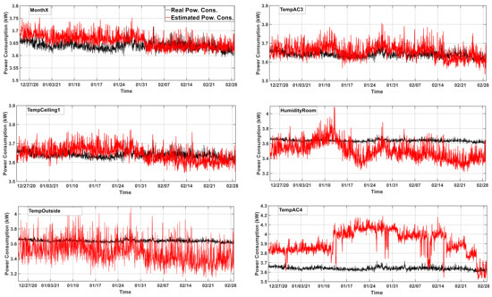
Figure 4.
The results of the power-consumption estimation performed using predictor pairs.
2.6.3. Experiment 3: The Best Combination of Predictors
After determining the second predictor based on the outcome of the previous experiment, in this experiment, a similar procedure was used to identify the third predictor. In addition to the predictors CpuMeanUsageRatio and MonthX, the forecasting procedure was repeated for the cases in which the remaining variables were used individually as the third predictor. After determining the third predictor, the same approach was continued to determine the other predictors until the error metrics no longer changed. The results are shown in Table 5 and Figure 5.
Table 5.
Error metrics for the estimation conducted using the best combination of predictors.
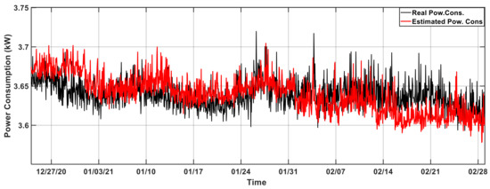
Figure 5.
The result of the power-consumption estimation of ARGE rack performed using the best combination of predictors.
3. Results and Discussion
In this section, the correlation analysis is carried out by mainly interpreting important relationships between variables for the correlation matrix shown in Figure 2. Afterwards, the results of experiments 1, 2, and 3 are sequentially presented.
3.1. Results of Correlation Analysis
The correlation coefficient, which ranges from −1 to +1, is a measure of the relationship between two variables [24]. As a rule of thumb, correlation coefficients close to 0 suggest a weak relationship between the variables, whereas correlation coefficients close to +1 or −1 imply significant relationships. In order to analyze the correlation between the variables, the correlation matrix was created by calculating the Pearson correlation coefficients in Matlab and is shown in Figure 2. The coefficient values of 0 are shown as white. Positive values up to +1 are shown as shades of green ranging from light to dark, whereas negative values up to −1 are shown from light red to dark red. According to Figure 2, the variable that correlated the most with the TotalPowerCons was MonthX, followed by CpuMeanUsageRatio, TempAC2, HumidityRoom, and TempOutside. The ones that correlated the least were TempAC1 and TempAC3, with a correlation value of −0.23 and 0.23, respectively. The variable of NetworkLoad, which was expected to have a high impact on the TotalPowerCons, was found to have a correlation value of 0.3, making it the variable with the third lowest correlation to TotalPowerCons. Furthermore, it was evident that there was quite an important correlation between CpuMeanUsageRatio and the variables MonthX, TempAC2, and RamMeanUsageRatio. Additionally, MonthX had a good correlation with almost all variables except TempAC1, TempAC3, FrontTopTemp, and NetworkLoad.
The highest correlation coefficient amongst all variables belonged to the relationship of TempAC4 to FrontTopTemp, with a correlation coefficient of 0.89. Surprisingly, TempAC1 and TempAC2, which were the airflow temperatures of the air conditioners in the GreenDC, did not have a correlation with TempCeiling1, TempCeiling2, or TempCeiling3, which are measuring the inside temperature of the GreenDC. However, there was quite a good correlation between TempAC3 with the variables of TempCeiling. NetworkLoad is the variable that had the lowest correlation with other variables. It only correlated with the variable of TotalPowerCons, with a correlation coefficient of 0.3.
3.2. Results of Experiment 1
The values of the different error metrics obtained as a result of the power-consumption estimation using each variable as a predictor individually are given in Table 3. The variables in the table are listed in descending order of MAPE values. Likewise, when the other metrics were used to compare the accuracy of the estimation results, a similar pattern was observed, except for MSE and RMSE. On the other hand, the error rates were compared according to MSE and RMSE, and although the best and worst results were the same, there was only a difference in the order of the results obtained for TempAC3 and RamMeanUsageRatio, and TempCeiling2 and TempAC2.
As can be seen from Table 3, the estimation result using only CpuMeanUsageRatio had the highest error value, although there was a high correlation between CpuMeanUsageRatio and TotalPowerCons. Similarly, even though the coefficient value of TempAC4 was higher than the values of TempAC1 and TempAC3, the error rate when the estimation was carried out with TempAC4 was higher than others. Graphs of the estimation results that were obtained using each variable as a predictor in Table 2 are shown in Figure 3.
As can be seen, the estimated value sometimes could not be used due to its inappropriate data characteristic, even if the MAPE value was low. For instance, the error rate of the estimation carried out with MonthX was very low. This is due to the fact that the estimation result remained a constant value for all days of the same month in the form of the step-function characteristic of MonthX. Likewise, the wave characteristics of the estimation result (HumidityRoom) with the second lowest error rate remained almost steady throughout the day and only slight changes occurred day to day. Additionally, the results of experiments carried out by using the variables RamMeanUsageRatio, TempCeiling3, and NetworkLoad remained steady instead of changing at each time step. On the other hand, the estimation result obtained using CpuMeanUsageRatio seemed to follow real power-consumption data, but it had the highest error rate.
This experiment also showed that the trend and characteristics of the estimated variable obtained were similar to those of the predictor when the estimation was carried out with only one predictor. This type of estimation result cannot be used because the most appropriate result should be estimated for each estimation interval instead of a constant value. Thus, it is not the best strategy to focus solely on the error metric and choose the one with the lowest value while making an estimation. The trend and characteristics of the estimated variable are also important and should be taken into account.
Furthermore, the relationship between the predictors often affects the estimation result. Even though the correlation coefficient is low and decreases the estimation accuracy when used alone, there may be variables that have a favourable impact on reducing the error rates when used together with another parameter. To analyze these types of cases, the second experiment was conducted.
3.3. Results of Experiment 2
Although the CpuMeanUsageRatio led to obtaining a bad estimation result when used alone, in Experiment 2, it was determined as the first predictor affecting power-consumption estimation of the ARGE rack because it is one of the most used predictors in the literature and is responsible for a large portion of the servers’ power consumption. The estimation process was repeated using other parameters one by one together with the CpuMeanUsageRatio, and accordingly, the changes in the accuracy of estimation results are given in Table 4. The variables in the table are organized in descending order of MAPE values. The order according to the estimation-error rate caused by predictor pairs was the same for all error metrics except for the predictor pairs of FrontTopTemp–CpuMeanUsageRatio and TempAC1–CpuMeanUsageRatio. According to the values of MSE and RMSE, the estimation result obtained by the predictor pairs FrontTopTemp–CpuMeanUsageRatio was better than that of TempAC1–CpuMeanUsageRatio, whereas it was worse than the predictor pairs of TempAC1–CpuMeanUsageRatio for the rest of the error metrics.
It is clear from Table 4 that the best estimation accuracy was obtained as a result of using CpuMeanUsageRatio and MonthX as predictors, whereas the worst one belonged to TempAC4 and CpuMeanUsageRatio. The MAPE value of the worst estimation result was 7.58%, whereas that of the best estimation result was 0.79%. In other words, the best estimation result was 90% lower than the worst estimation result. Moreover, the value of the correlation coefficient between TemAC4 and TotalPowerCons was almost twice that of TempAC3, yet the estimation result obtained with TempAC4 was almost eight times worse than that of TempAC3. Despite the fact that TempAC3 was one of the variables with the lowest correlation coefficient with TotalPowerCons and did not correlate with CpuMeanUsageRatio, it provided the second-best estimation result when used with CpuMeanUsageRatio. Other surprising results were obtained with the variables TempOutside and HumidityRoom, which had a high correlation with TotalPowerCons. They led to the second and third worst results, respectively. The results of each case of Experiment 2 are also shown graphically in Figure 4. The estimation-result graph belonging to the pair MonthX–CpuMeanUsageRatio was the most appropriate graph, and it also had the lowest error rate.
When the remaining graphs were examined, it was clear that the trends of the result graphs changed according to the increase in error rates. The graphs belonging to the pairs TempAC3–CpuMeanUsageRatio and TempCeiling1–CpuMeanUsageRatio, which had the second and third lowest error rates, also had acceptable trends and characteristics. Similarly, the three worst estimation results in terms of error rate, which belonged to the pairs CpuMeanUsageRatio–HumidityRoom, TempOutside, and TempAC4, were also graphically unacceptable. At the end of this experiment, MonthX was determined to be the second predictor in the power-estimation model of the ARGE rack.
3.4. Results of Experiment 3
In this experiment, a similar approach as in experiment 2 was followed to find the best combination of predictors that yielded the best estimation result. To determine the third and other predictors, all variables except CpuMeanUsageRatio and MonthX were used individually and the results were analyzed. At the end of the experiment, NetworkLoad, and TempAC3 were determined to be the third and fourth predictors, respectively, despite the fact that they had a limited influence on the estimation results when employed alone and had low correlation coefficients. On the contrary, it was decided that the RamMeanUsageRatio variable, which had a pretty high correlation coefficient and provided a relatively good estimation result when used together with the CpuMeanUsageRatio, could not be used. When RamMeanUsageRatio was used as a third, fourth, or fifth predictor, it always led to an increase in the error rates. Furthermore, although it was found in the second experiment that TempOutside increased the error rate, this experiment demonstrated that it reduced the estimation error when used with other predictors. As a consequence, the best predictor combination and the value of different error metrics obtained when the estimation was carried out with these predictors are shown in Table 5. Additionally, the estimated results are shown in Figure 5 graphically.
When the MAPE values of the estimation results obtained using only CpuMeanUsageRatio as a predictor and the best combination of predictors were compared, it was seen that the ratio of MAPE was reduced from 5.79% to 0.53% with an improvement of almost 10 times. This improvement rate was almost the same when the comparison was carried out with the error metrics of MAE, RMSPE, sMAPE, and MASE.Additionally, it was observed that the error rate improved by nine times in the comparison made according to RMSE and by 90 times in the comparison made according to MSE. Figure 5 shows the estimation result obtained using the best combination of predictors.
4. Conclusions
The feature-/predictor-selection process plays a critical role in load forecasting. In addition, conducting experiments with the data measured under real working conditions is very important for the relevance and reliability of the results, especially in the estimation processes in which the workload characteristics affect the server power consumption in a data center. Even though many studies have employed various methodologies and approaches for feature/predictor selection, there is a lack of research on predictor selection by analyzing the direct effect of predictors on the estimation result. In this paper, the predictors’ effects on the power consumption of the ARGE rack were investigated via three different experiments using actual data measured from IoT-based sensors and the ARGE rack, which were operating under real-world workloads.
In order to investigate the individual effect of predictors on power-consumption estimation of the ARGE rack, the estimation was carried out using only one variable as a predictor from the probable predictor set in Experiment 1.
The CpuMeanUsageRatio was determined to be the first predictor because it is one of the most popular variables used in the literature for power-consumption estimation of servers. The remaining variables apart from CpuMeanUsageRatio were determined as the second predictor used one by one, and the estimation process was repeated for each case in Experiment 2.
In Experiment 3, a similar approach was followed to determine the best combination of predictors in order to obtain accurate and reliable estimation results. According to the conducted experiments and analyses, the following conclusions can be derived.
- As a consequence of the correlation analysis, although CpuMeanUsageRatio had quite a high correlation with TotalPowerCons, it had the highest estimation error rate. Similarly, TempAC4 had a higher correlation-coefficient value than TempAC1 and TempAC3. However, when each of them was utilized for the estimation, TempAC4 caused the greatest estimation-error rate. Therefore, it should not be generalized that a variable that has a higher correlation coefficient than others improves the estimation accuracy or vice versa.
- According to error metrics obtained from experiment 1, the usage of CpuMeanUsageRatio individually as a predictor resulted in the worst estimation error among all other variables, whereas MonthX caused the best result. However, the estimation result carried out using MonthX could not be used because the data characteristic and trend of the result were not appropriate. So, determining the predictor solely by examining the error metric is not sufficient to obtain a suitable estimation result; the trend and characteristics of the estimated variable should also be considered.
- Experiment 2 showed that some variables with a low correlation coefficient might improve the estimation accuracy when combined with other variables, although they cause poor estimation accuracy when used alone. For instance, TempAC3, although having one of the lowest correlation coefficients with TotalPowerCons, caused the second-best estimation result when combined with CpuMeanUsageRatio. Furthermore, TempOutside reduced the estimation error when utilized with CpuMeanUsageRatio, Monthx, NetworkLoad, and TempAC3 in Experiment 3 in contrast to Experiment 2, in which the second-worst estimation result was obtained by usage of CpuMeanUsageRatio and TempOutside. This was due to the correlation between TempOutside to the other variables.
- Despite the fact that CPU usage is a very important variable for a server, and many studies have derived CPU-based power-consumption models and carried out estimations, this study demonstrated that estimation by incorporating additional variables together with the CpuMeanUsageRatio provides more accurate and reliable estimation results. In this study, the most reliable and accurate estimation result of the power consumption of the ARGE rack was obtained using the predictors CpuMeanUsageRatio, MonthX, NetworkLoad, TempAC3, and TempOutside with a MAPE ratio of 0.53%, which was 10 times better than the MAPE ratio obtained using solely CpuMeanUsageRatio.
Consequently, this study shows that rather than determining predictors using only one perspective or one method in an estimation process, it is necessary to choose them by making a comparative analysis, investigating their effects on estimation results, and examining the trend and characteristics of the estimated variable. This approach provides accurate and reliable estimation results while avoiding the use of redundant predictors. Thus, not only is the cost and effort of measuring redundant variables reduced but the execution time for training and estimation is also sped up because fewer variables are used. The findings of this study will be beneficial while developing estimation models for power consumption in several studies pertaining to energy management and efficiency, particularly in data centers, which have grown in prominence as a result of the COVID-19 pandemic. Additionally, it will also be very useful in studies related to load forecasting and feature selection. In the future, the proposed approach for predictor selection can be modelled and formulated as a hybrid feature-selection method. The experiments can be extended to determine predictors for power-consumption estimation of a whole data center so as to compare the effectiveness of this new method on estimation accuracy and execution time with other feature-selection methods.
Author Contributions
Conceptualization, M.T.T. and T.G.; methodology, analysis, and writing—original draft preparation, M.T.T.; writing—review and editing, M.T.T. and T.G.; supervision, T.G. All authors have read and agreed to the published version of the manuscript.
Funding
This work was supported in part by the GREENDC project from the European Union’s Horizon 2020 research and innovation program under the Marie Skłodowska-Curie grant agreement No. 734273.
Institutional Review Board Statement
Not applicable.
Informed Consent Statement
Not applicable.
Data Availability Statement
Not applicable.
Conflicts of Interest
The authors declare no conflict of interest.
Nomenclature
| TempAC1, TempAC2, TempAC3, TempAC4 | Airflow temperatures of air conditioners in four different locations. |
| TempCeiling1, TempCeiling2, TempCeiling3 | Indoor temperatures of three different locations on the ceiling of the data center. |
| TempOutside | Mean outside temperature |
| CpuMeanUsageRatio | The mean of 10 servers’ CPU-usage ratios in the ARGE rack |
| RamMeanUsageRatio | The mean of 10 servers’ RAM-usage ratios in the ARGE rack |
| FrontTopTemp | The temperature of the top of the front door of the ARGE rack |
| NetworkLoad | The total in/out network-traffic load |
| HumidityRoom | Mean room humidity of the data center |
| MonthX | Sine parts of month data |
| MonthY | Cosines parts of month data |
| TotalPowerCons | The total power consumption of 10 servers in the ARGE rack |
| The order of the month in a year | |
| Power consumption of the ARGE rack | |
| MSE | Mean square error |
| RMSE | Root mean square error |
| MAE | Mean absolute error |
| MAPE | Mean absolute percentage error |
| RMSPE | Root mean square percentage error |
| sMAPE | Symmetric mean absolute percentage error |
| MASE | Mean absolute scaled error |
References
- Cisco Establishing the Edge—A New Infrastructure Model for Service Providers. Available online: https://www.cisco.com/c/en/us/solutions/service-provider/edge-computing/establishing-the-edge.html (accessed on 31 August 2021).
- Yu, W.; Liang, F.; He, X.; Hatcher, W.G.; Lu, C.; Lin, J.; Yang, X. A Survey on the Edge Computing for the Internet of Things. IEEE Access 2017, 6, 6900–6919. [Google Scholar] [CrossRef]
- Takci, M.T.; Gozel, T.; Hocaoglu, M.H. Forecasting Power Consumption of IT Devices in a Data Center. In Proceedings of the 20th International Conference on Intelligent System Application to Power Systems, ISAP 2019, New Delhi, India, 10–14 December 2019; pp. 1–8. [Google Scholar]
- Hafeez, G.; Alimgeer, K.S.; Qazi, A.B.; Khan, I.; Usman, M.; Khan, F.A.; Wadud, Z. A Hybrid Approach for Energy Consumption Forecasting with a New Feature Engineering and Optimization Framework in Smart Grid. IEEE Access 2020, 8, 96210–96226. [Google Scholar] [CrossRef]
- Song, H.; Qin, A.K.; Salim, F.D. Evolutionary Multi-Objective Ensemble Learning for Multivariate Electricity Consumption Prediction. In Proceedings of the International Joint Conference on Neural Networks (IJCNN), Rio de Janeiro, Brazil, 8–13 July 2018; pp. 1–8. [Google Scholar]
- Pirbazari, A.M.; Chakravorty, A.; Rong, C. Evaluating Feature Selection Methods for Short-Term Load Forecasting. In Proceedings of the IEEE International Conference on Big Data and Smart Computing, Kyoto, Japan, 27 February–2 March 2019; pp. 1–8. [Google Scholar]
- Baig, S.U.R.; Iqbal, W.; Berral, J.L.; Erradi, A.; Carrera, D. Adaptive Prediction Models for Data Center Resources Utilization Estimation. IEEE Trans. Netw. Serv. Manag. 2019, 16, 1681–1693. [Google Scholar] [CrossRef]
- Jin, C.; Bai, X.; Yang, C.; Mao, W.; Xu, X. A Review of Power Consumption Models of Servers in Data Centers. Appl. Energy 2020, 265, 114806. [Google Scholar] [CrossRef]
- Takcı, M.T.; Gözel, T.; Hocaoğlu, M.H. Quantitative Evaluation of Data Centers’ Participation in Demand Side Management. IEEE Access 2021, 9, 14883–14896. [Google Scholar] [CrossRef]
- Cupelli, L.; Schutz, T.; Jahangiri, P.; Fuchs, M.; Monti, A.; Muller, D. Data Center Control Strategy for Participation in Demand Response Programs. IEEE Trans. Ind. Inform. 2018, 14, 5087–5099. [Google Scholar] [CrossRef]
- Guo, Y.; Li, H.; Pan, M. Colocation Data Center Demand Response Using Nash Bargaining Theory. IEEE Trans. Smart Grid 2018, 9, 4017–4026. [Google Scholar] [CrossRef]
- Fridgen, G.; Keller, R.; Thimmel, M.; Wederhake, L. Shifting Load through Space—The Economics of Spatial Demand Side Management Using Distributed Data Centers. Energy Policy 2017, 109, 400–413. [Google Scholar] [CrossRef]
- Vasques, T.L.; Moura, P.; de Almeida, A. A Review on Energy Efficiency and Demand Response with Focus on Small and Medium Data Centers. Energy Effic. 2019, 12, 1399–1428. [Google Scholar] [CrossRef]
- Zhou, Z.; Abawajy, J.H.; Li, F.; Hu, Z.; Chowdhury, M.U.; Alelaiwi, A.; Li, K. Fine-Grained Energy Consumption Model of Servers Based on Task Characteristics in Cloud Data Center. IEEE Access 2017, 6, 27080–27090. [Google Scholar] [CrossRef]
- Lin, W.; Wu, G.; Wang, X.; Li, K. An Artificial Neural Network Approach to Power Consumption Model Construction for Servers in Cloud Data Centers. IEEE Trans. Sustain. Comput. 2020, 5, 329–340. [Google Scholar] [CrossRef]
- Jawad, M.; Qureshi, M.B.; Khan, M.U.S.; Ali, S.M.; Mehmood, A.; Khan, B.; Wang, X.; Khan, S.U. A Robust Optimization Technique for Energy Cost Minimization of Cloud Data Centers. IEEE Trans. Cloud Comput. 2021, 9, 447–460. [Google Scholar] [CrossRef]
- Pelley, S.; Meisner, D.; Wenisch, T.F.; VanGilder, J.W. Understanding and Abstracting Total Data Center Power. In Proceedings of the Workshop on Energy Efficient Design, Austin, TX, USA, 25 January 2009. [Google Scholar]
- Hsu, Y.F.; Matsuda, K.; Matsuoka, M. Self-Aware Workload Forecasting in Data Center Power Prediction. In Proceedings of the 18th IEEE/ACM International Symposium on Cluster, Cloud and Grid Computing, Washington, DC, USA, 1–4 May 2018; pp. 321–330. [Google Scholar]
- Wang, K.; Xu, C.; Zhang, Y.; Guo, S.; Zomaya, A.Y. Robust Big Data Analytics for Electricity Price Forecasting in the Smart Grid. IEEE Trans. Big Data 2017, 5, 34–45. [Google Scholar] [CrossRef]
- Liang, Y.; Hu, Z. Prediction Method of Energy Consumption Based on Multiple Energy-Related Features in Data Center. In Proceedings of the IEEE International Conference on Parallel & Distributed Processing with Applications, Big Data & Cloud Computing, Sustainable Computing & Communications, Social Computing & Networking, Xiamen, China, 16–18 December 2019; pp. 140–146. [Google Scholar]
- Yu, X.; Zhang, G.; Li, Z.; Liangs, W.; Xie, G. Toward Generalized Neural Model for VMs Power Consumption Estimation in Data Centers. In Proceedings of the ICC 2019-2019 IEEE International Conference on Communications, Shanghai, China, 20–24 May 2019. [Google Scholar]
- Koprinska, I.; Rana, M.; Agelidis, V.G. Correlation and Instance Based Feature Selection for Electricity Load Forecasting. Knowl. Based Syst. 2015, 82, 29–40. [Google Scholar] [CrossRef]
- Billah Kushal, T.R.; Illindala, M.S. Correlation-Based Feature Selection for Resilience Analysis of MVDC Shipboard Power System. Int. J. Electr. Power Energy Syst. 2020, 117, 105742. [Google Scholar] [CrossRef]
- Chen, P.Y.; Popovich, P.M. Correlation: Parametric and Nonparametric Measures; SAGE Publications: London, UK, 2011. [Google Scholar]
- Yao, J.; Liu, X.; He, W.; Rahman, A. Dynamic Control of Electricity Cost with Power Demand Smoothing and Peak Shaving for Distributed Internet Data Centers. In Proceedings of the 2012 IEEE 32nd International Conference on Distributed Computing Systems, Macau, China, 18–21 June 2012; pp. 416–424. [Google Scholar] [CrossRef]
- Roy, S.; Rudra, A.; Verma, A. An Energy Complexity Model for Algorithms. In Proceedings of the 4th conference on Innovations in Theoretical Computer Science, Berkeley, CA, USA, 10–12 January 2013; p. 283. [Google Scholar]
- Daraghmeh, M.; al Ridhawi, I.; Aloqaily, M.; Jararweh, Y.; Agarwal, A. A Power Management Approach to Reduce Energy Consumption for Edge Computing Servers. In Proceedings of the 2019 4th International Conference on Fog and Mobile Edge Computing, FMEC, Rome, Italy, 10–13 June 2019; pp. 259–264. [Google Scholar] [CrossRef]
- Berezovskaya, Y.; Yang, C.W.; Mousavi, A.; Vyatkin, V.; Minde, T.B. Modular Model of a Data Centre as a Tool for Improving Its Energy Efficiency. IEEE Access 2020, 8, 46559–46573. [Google Scholar] [CrossRef]
- Radulescu, C.Z.; Radulescu, D.M. A Performance and Power Consumption Analysis Based on Processor Power Models. In Proceedings of the 12th International Conference on Electronics, Computers and Artificial Intelligence, ECAI, Bucharest, Romania, 25–27 June 2020; pp. 38–41. [Google Scholar]
- Wang, S.; Zhang, Z. Short-Term Multiple Load Forecasting Model of Regional Integrated Energy System Based on Qwgru-Mtl. Energies 2021, 14, 6555. [Google Scholar] [CrossRef]
- Gao, X.; Li, X.; Zhao, B.; Ji, W.; Jing, X.; He, Y. Short-Term Electricity Load Forecasting Model Based on EMD-GRU with Feature Selection. Energies 2019, 12, 1140. [Google Scholar] [CrossRef]
- Pallonetto, F.; Jin, C.; Mangina, E. Forecast Electricity Demand in Commercial Building with Machine Learning Models to Enable Demand Response Programs. Energy AI 2022, 7, 100121. [Google Scholar] [CrossRef]
- Han, X.; Su, J.; Hong, Y.; Gong, P.; Zhu, D. Mid-to Long-Term Electric Load Forecasting Based on the EMD–Isomap–Adaboost Model. Sustainability 2022, 14, 7608. [Google Scholar] [CrossRef]
- Huang, Y.; Zhao, R.; Zhou, Q.; Xiang, Y. Short-Term Load Forecasting Based on a Hybrid Neural Network and Phase Space Reconstruction. IEEE Access 2022, 10, 23272–23283. [Google Scholar] [CrossRef]
- Lin, L.; Xue, L.; Hu, Z.; Huang, N. Modular Predictor for Day-Ahead Load Forecasting and Feature Selection for Different Hours. Energies 2018, 11, 1899. [Google Scholar] [CrossRef]
- Forootani, A.; Rastegar, M.; Sami, A. Short-Term Individual Residential Load Forecasting Using an Enhanced Machine Learning-Based Approach Based on a Feature Engineering Framework: A Comparative Study with Deep Learning Methods. Electr. Power Syst. Res. 2022, 210, 108119. [Google Scholar] [CrossRef]
- Yousaf, A.; Asif, R.M.; Shakir, M.; Rehman, A.U.; Adrees, M.S. An Improved Residential Electricity Load Forecasting Using a Machine-Learning-Based Feature Selection Approach and a Proposed Integration Strategy. Sustainability 2021, 13, 6199. [Google Scholar] [CrossRef]
- Yang, L.; Yang, H.; Yang, H.; Liu, H. GMDH-Based Semi-Supervised Feature Selection for Electricity Load Classification Forecasting. Sustainability 2018, 10, 217. [Google Scholar] [CrossRef]
- Bouktif, S.; Fiaz, A.; Ouni, A.; Serhani, M.A. Optimal Deep Learning LSTM Model for Electric Load Forecasting Using Feature Selection and Genetic Algorithm: Comparison with Machine Learning Approaches. Energies 2018, 11, 1636. [Google Scholar] [CrossRef]
- Pei, S.; Qin, H.; Yao, L.; Liu, Y.; Wang, C.; Zhou, J. Multi-Step Ahead Short-Term Load Forecasting Using Hybrid Feature Selection and Improved Long Short-Term Memory Network. Energies 2020, 13, 4121. [Google Scholar] [CrossRef]
- Subbiah, S.S.; Chinnappan, J. Deep Learning Based Short Term Load Forecasting with Hybrid Feature Selection. Electr. Power Syst. Res. 2022, 210, 108065. [Google Scholar] [CrossRef]
- Liu, R.; Chen, T.; Sun, G.; Muyeen, S.M.; Lin, S.; Mi, Y. Short-Term Probabilistic Building Load Forecasting Based on Feature Integrated Artificial Intelligent Approach. Electr. Power Syst. Res. 2022, 206, 107802. [Google Scholar] [CrossRef]
- Takcı, M.T.; Gözel, T.; Hocaoğlu, M.H.; Öztürk, O.; Lee, H.; Yovchev, S. Deliverable D2.1: Design of the GREENDC DSS. In Sustainable Energy Demand Side Management for GREEN Data Centers (GreenDC); European Commission: Brussels, Belgium, 2017. [Google Scholar] [CrossRef]
- Botchkarev, A. Performance Metrics (Error Measures) in Machine Learning Regression, Forecasting and Prognostics: Properties and Typology. arXiv 2018, arXiv:1809.03006. [Google Scholar]
- Hyndman, R.J.; Koehler, A.B. Another Look at Measures of Forecast Accuracy. Int. J. Forecast. 2006, 22, 679–688. [Google Scholar] [CrossRef]


Publisher’s Note: MDPI stays neutral with regard to jurisdictional claims in published maps and institutional affiliations. |
© 2022 by the authors. Licensee MDPI, Basel, Switzerland. This article is an open access article distributed under the terms and conditions of the Creative Commons Attribution (CC BY) license (https://creativecommons.org/licenses/by/4.0/).