Abstract
Reverse logistics is attracting attention due to the increasing concerns over environmental issues and the important economic impacts. The design of a reverse logistics network is a major strategic problem in the field of reverse logistics. As cost pressures in product returns continue to mount, a growing number of manufacturers have begun to outsource reverse logistics operations to third-party logistics (3PL) providers. On the other hand, considering disruption risks caused by natural or man-made factors in the reverse logistics network design is inevitable. This paper studies third-party reverse logistics network designs under uncertain disruptions. The problem is formulated as a risk-averse two-stage stochastic programming model with a mean risk objective. Two types of risk measures, value at risk (VaR) and conditional value at risk (CVaR), were examined, respectively. Finally, the sensitivity analysis of the model was carried out. The validity of the mean risk criteria is proved by comparison with risk-neutral approach. Moreover, the performance of the proposed model was examined by stochastic measures.
1. Introduction
In recent decades, the development of humanity has led to unfavorable climate changes and natural disasters [1]. More attention has been placed on sustainability development to prompt socioeconomic development in line with ecological constraints [2]. In recent two decades, due to increasing environmental concerns and economic benefits, many companies have focused on reverse logistics [3]. Reverse logistics can be described as the process of collecting returned products from the customers to the manufacturers to capture appropriate disposal activities [4]. However, reverse logistics operations are extremely complicated and are out of companies’ technological scopes. Due to the uncertainties surrounding the quantity and time of product returns, reverse logistics usually require specialized infrastructure and high handling costs and time [5]. Currently, many companies have inefficient processes for returned products. In addition, the implementations of return operations require high investments in equipment, recovery processes, information systems, etc., which are not core capacities of manufacturers [6]. In contrast, 3PL can save a substantial amount of costs associated with product returns through their complete RL networks, advanced equipment, substantial operational experiences, and required information systems [7]. Therefore, more companies have begun to outsource their reverse logistics to 3PL providers. Reverse logistics network design, as one of the most important strategic decision problems, plays a key role in the effective operation of reverse logistics. Consequently, it is significant for 3PL providers to design an efficient reverse logistics network for their clients.
Disruption risk has become a hot topic in the field of supply chain network design [8,9]. Most studies on reverse logistics network designs assume that facilities are always available. However, sometimes facilities may be unavailable due to the disruptions caused by natural or man-made disasters, such as hurricanes, earthquakes, and terrorist attacks, which might pose destructive impacts on the reverse logistics network. Therefore, it is important to consider disruption risk when designing a reverse logistics network. Moreover, most of the existing works on the supply chain network design with disruptions utilize risk-neutral approaches to address the uncertainty of disruptions [10]. Nevertheless, for non-repeatable decision-making problems, the risk management method can more effectively control the uncertainty in the optimization problem. The literature studies on reverse logistics network design also suffer from a lack of models that are able to measure and control the disruption risks. Therefore, it is necessary to design reverse logistics networks under disruptions (for 3PL) via the risk management method.
This study proposes a risk-averse model for designing a reverse logistics network for 3PL under uncertain disruptions. In this problem, a manufacturer outsources its reverse logistics activities to a 3PL provider. The reverse logistics network includes customer zones, 3PL local collection centers, 3PL centralized collection centers, plants, and disposal centers. A risk-averse two-stage stochastic programming model was developed. The objective of the model is to minimize the mean risk function, where CVaR and VaR are taken as the risk measures, respectively. In order to verify the validity of the proposed risk-averse models, some numerical experiments were executed. Moreover, the effects of the parameters on the performance of the model were analyzed.
The rest of this article is organized as follows: the relevant literature is reviewed in Section 2. The problem with the reverse logistics network design for 3PL (under uncertain disruptions) is described and risk-averse two-stage stochastic programming modes with mean risk objectives are presented in Section 3. The numeric experiment was conducted to analyze the effects of the important parameters and demonstrate the validity of the model in Section 4. Finally, the study is concluded in Section 5.
2. Literature Review
In this section, a summary of the most relevant papers in this area is presented. The studies can be divided into the following three categories:
2.1. Reverse Logistics Network Design for 3PL Providers
The reverse logistics network design problem has received considerable attention in the past two decades. The studies on reverse logistics network design have been surveyed [3,11,12]. However, there are only a few works addressing the problem with the reverse logistics network design for 3PL. Mahmoudzadeh et al. [6] proposed a mixed-integer linear programming (MILP) model for the reverse logistics network design of end-of-life vehicles for 3PL in Iran to determine optimal locations of scrap yards and material flows. Suyabatmaz et al. [13] presented a hybrid simulation–analytical modeling framework for the reverse logistics network design of 3PL under uncertainty. Kannan et al. [14] considered the reverse logistics network design problem, which integrated a balanced disassembly line for 3PL. They formulated the problem as a mixed-integer non-linear programming (MINLP) model to optimize the total cost. Eskandarpour et al. [15] proposed a bi-objective MILP model for the 3PL multi-product post-sale network design problem to minimize the total cost and total weighted tardiness of returning repaired and new products. They developed a novel variable neighborhood search algorithm to solve the problem. Min and Ko [16] developed a MINLP model for the 3PL dynamic reverse logistics network design problem to determine the location and allocation of repair facilities. They proposed a genetic algorithm to solve the problem. Du and Evans [17] considered a reverse logistics network design problem for the post-sales service of a manufacturer. They developed a bi-objective optimization model for designing a reverse logistics network to minimize the costs and tardiness of the cycle time. In addition, a few papers have attended to integrate forward and reverse logistics network designs for 3PL providers, e.g., [5,18,19,20,21]. To the best of our knowledge, no study considers disruption risk in the context of reverse logistics network design for 3PL.
2.2. Stochastic Reverse Logistics Network Design
Several works have attempted to develop stochastic models for reverse logistics network design problems under uncertainty. Ayvaz et al. [22] developed a two-stage stochastic programming model to design a reverse logistics network for third-party waste of electrical and electronic equipment (from recycling companies) with stochastic return quantities, sorting ratios, and transportation costs. The objective of the model was to maximize profit. They employed the sample average approximation method to solve the problem. Trochu et al. [23] considered reverse logistics network design under uncertainty with dynamic supply source locations. They presented a two-stage stochastic programming model to maximize the expected profit. Yu and Solvang [24] proposed a two-stage stochastic mixed-integer linear programming model for sustainable multi-product multi-echelon reverse logistics design under uncertainty. The objective of the model was to maximize the profit with carbon emission constraints. They presented a multi-criteria scenario-based risk-averse solution method for solving the proposed model. Kara and Onut [4] presented a reverse logistics network design under uncertainty for recycling/manufacturing types of systems in a reverse supply chain. They proposed a two-stage stochastic programming model to decide the optimal recycling and collection center locations and optimal flow amounts between the nodes. Fonseca et al. [25] studied multiple echelons, multiple commodities, and reverse logistics network designs with stochastic transportation costs and waste generation. They formulated the problem as a bi-objective two-stage stochastic programming model to minimize the total cost and the obnoxious effects caused by the reverse network facilities. Yu and Solvang [26] presented a bi-objective two-stage stochastic programming model to design a sustainable multi-product multi-echelon reverse logistics system under uncertainty. In the model, they considered profitability and environmental performance with flexible capacity. Roudbari et al. [27] proposed a two-stage stochastic programming model for designing a reverse logistics network with uncertain quality and quantity of returned products, product variety, and a bill of material. In the model, various processes of recovering recyclable products were considered. They developed a hybrid algorithm to solve the model. Fattahi and Govindan [28] addressed an integrated forward/reverse logistics network design problem in which demand and potential return uncertainty and multiple tactical periods were considered. The model was formulated in two-stage stochastic programming. They developed a novel simulation-based simulated annealing algorithm for solving large-sized test problems. Pishvaee et al. [29] formulated the integrated forward/reverse logistics network design under uncertainty by a scenario-based stochastic approach. The model minimizes the total expected costs. Vahdat and Vahdatzad [30] utilized two-stage stochastic programming to design a multi-period multistage integrated forward/reverse logistics network under uncertainty. They developed Benders’ decomposition to solve the problem.
2.3. Reverse Logistics Network Design under Disruption Risk
In the past two decades, a considerable amount of literature has been dedicated to the supply chain network design under disruptions [8,9]. However, the literature on the reverse logistics network design with disruption risk is still scarce. Sugimura and Murakami [31] proposed a MILP model for designing a resilient international reverse logistics network under disruptions. The objective of the model was to minimize the total costs with the resilience constraints. Govindan and Gholizadeh [32] studied a resilient sustainable reverse logistics network design for end-of-life vehicles in Iran, in which the network facility capacity was disrupted. They developed a robust optimization model to minimize the total costs. A scenario-based cross-entropy method was used to solve the proposed model. Some research studies have addressed the integrated forward and reverse logistics network design under uncertain disruption by a scenario-based stochastic method, including two-stage stochastic programming [33,34,35] and scenario-based robust optimization [36,37,38,39,40]. In fact, none of the above studies considered risk measures to cope with disruption uncertainties.
2.4. Incorporating Risk Measures in a Stochastic Reverse Logistics Network Design
Recently, risk management in a reverse logistics network design problem has received more attention. In the proposed models, different risk measures are used to control the risk level. Rahimi and Ghezavati [41] studied the network design problem for reverse logistics for recycling construction and demolition waste; the stochastic demand for recycled products and the rate of investment were considered. They proposed a multi-period–multi-objective MILP model. The objectives of the model were the maximization of profit, social impact, and minimization of environmental effects. A risk-averse two-stage stochastic programming based on CVaR was used to deal with the uncertainty in the model. Soleimani and Govindan [42] utilized a risk-averse two-stage stochastic programming approach to design a reverse supply chain network under uncertainty. In their model, a mean CVaR objective function was regarded. Ma et al. [43] proposed a new distributionally robust optimization model to design a multi-product, multi-echelon closed-loop supply chain network. In the model, mean CVaR was used as the objective function. Finally, they validated the proposed model through a case study. Soleimani et al. [44] studied the design and planning problem of a closed-loop supply chain network with uncertain parameters. They incorporated three risk measures into the mean risk objective function in the two-stage stochastic structure. Finally, the performances of the developed models were evaluated. Ramezani et al. [45] presented a stochastic multi-objective model for designing a forward/reverse logistic network under uncertainty. In this model, financial risk is defined as the probability of a determined objective where profit does not meet a certain target level. Fard et al. [46] developed a bi-objective stochastic programming model for a closed-loop supply chain network design problem. In the model, they optimized total costs and downside risks, simultaneously.
2.5. Research Gaps and Contributions
According to the above literature review and Table 1, it can be inferred that the reverse logistics network design problem under disruption risk for 3PL has not been addressed and that no study has considered the risk measures to cope with disruption uncertainties in reverse logistics network design problems. To the best of our knowledge, no study has considered uncertain disruptions and risk measures in the modeling of third-party reverse logistics network design problems.

Table 1.
Review of previously published literature.
The main contributions of this work can be summarized as follows:
- This study is the first to present a third-party reverse logistics network design problem considering disruptions and risk management simultaneously.
- For the first time, risk-averse two-stage stochastic programming models were developed to solve reverse logistics network designs under uncertain disruptions for 3PL.
- Two risk measures, CVaR and VaR, were investigated.
- A numerical example was used to analyze the performances of the risk-averse two-stage stochastic programming models.
3. Problem Description and Proposed Model
In this article, a multi-echelon reverse logistics network design problem of 3PL with uncertain disruption is presented. As shown in Figure 1, the reverse logistics network consists of customer zones, 3PL local collection centers, 3PL centralized collection centers, plants, disposal centers, and transportation links. Moreover, 3PL offers reverse logistics services for a manufacturer using its local collection centers and centralized collection centers. The returned products were collected from customer zones and conveyed to 3PL centralized collection centers via 3PL local collection centers. After testing, inspection, and sorting in 3PL centralized collection centers, the recoverable products were transported to plants, and non-recoverable products were disposed of in the disposal centers. Uncertain disruptions at 3PL local collection centers and 3PL centralized collection centers were considered. The goal of this study was to develop a risk-averse mathematical modeling framework to design a third-party reverse logistics network considering uncertain disruptions by determining 3PL local collection centers and 3PL centralized collection centers to be opened, as well as the quantities of products transported between facilities in each scenario.
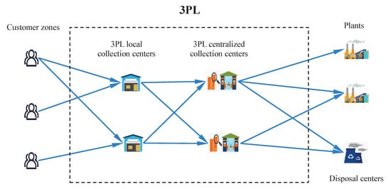
Figure 1.
Third-party reverse logistics network.
3.1. Assumptions
The main assumptions considered in the presented model are as follows:
- 1.
- Multi-echelon, consisting of customer zones, 3PL local collection centers, 3PL centralized collection centers, disposal centers, and plants are considered in the reverse network.
- 2.
- The locations, numbers, and return quantities of the products at the customer zones are known.
- 3.
- The locations, numbers, and capacities of the plants and disposal centers are known.
- 4.
- The potential locations, numbers, and capacities of 3PL local collection centers, 3PL centralized collection centers, and cost parameters (i.e., fixed opening costs, processing costs) are known.
- 5.
- Unit transportation costs for the product between the two adjacent echelons are known.
- 6.
- Penalty costs will be incurred for uncollected returned products.
- 7.
- The disruptions of the 3PL local collection centers and 3PL centralized collection centers are uncertain and can be described by the set of scenarios.
3.2. Notations
The following sets, parameters, and decision variables are used in the proposed models:
3.2.1. Sets
| L | Set of customer zones |
| K | Set of 3PL local collection centers |
| J | Set of 3PL centralized collection centers |
| I | Set of disposal centers |
| M | Set of plants of the manufacturer |
| S | Set of scenarios |
3.2.2. Parameters
| Quantity of returned products in customer zone l | |
| Unit processing cost of returned products at 3PL local collection center k | |
| Capacity of processing for 3PL local collection center k | |
| Fixed opening cost of 3PL local collection center k | |
| Unit processing cost of returned products at 3PL centralized collection center j | |
| Capacity of processing for 3PL centralized collection center j | |
| Fixed opening cost of 3PL centralized collection center j | |
| Capacity of disposal for disposal center i | |
| Capacity of production for plant m | |
| Unit transportation cost for products shipped from customer zone l to 3PL local collection center k | |
| Unit transportation cost for products shipped from 3PL local collection center k to 3PL centralized collection center j | |
| Unit transportation cost for products shipped from the 3PL centralized collection center j to disposal center i | |
| Unit transportation cost for products shipped from the 3PL centralized collection center j to plant m | |
| Unit penalty cost for the uncollected returned products | |
| Disposal ratio of products at 3PL centralized collection center | |
| Probability of disruption scenario s |
3.2.3. Decision Variables
| Binary variable equals 1 if 3PL local collection center k is opened and 0 otherwise | |
| Binary variable equals 1 if 3PL centralized collection center j is opened and 0 otherwise | |
| Quantity of products shipped from customer zone l to 3PL local collection center k in scenario s | |
| Quantity of products shipped from 3PL local collection center k to 3PL centralized collection center j in scenario s | |
| Quantity of products shipped from the 3PL centralized collection center j to disposal center i in scenario s | |
| Quantity of products shipped from the 3PL centralized collection center j to plant m in scenario s |
The and denote the vectors of the respective decision variables, where and .
3.3. Risk-Neutral Two-Stage Stochastic Programming Model
In terms of the above notations, the risk-neutral two-stage stochastic programming model can be formulated as follows:
s.t.
The objective function (1) minimizes the expected total cost of the logistics network, including the fixed opening costs of 3PL local collection centers and 3PL centralized collection centers, as well as the expected operation costs. indicates the operation costs of the network in scenario s, including the processing and transportation costs of the returned products, and the penalty costs for uncollected returned products. Indeed, is the optimal value of the second-stage problem and it is illustrated as follows:
s.t.
Equations (2) and (3) are related to the binary restrictions of the first-stage decision variables. Constraints (5) and (6) ensure the flow balance at 3PL local collection centers and 3PL centralized collection centers. Constraint (7) indicates that the disposal ratio of the returned products at each 3PL centralized collection center is . Constraint (8) means that the products shipped out of a customer zone cannot exceed the return quantity. Equation (9) is the capacity constraint of 3PL local collection centers and prohibits the products from being transferred into 3PL local collection centers, which are not opened or disrupted, where if the 3PL local collection center k is disrupted in scenario s, and otherwise. Equation (10) is the capacity constraint of 3PL centralized collection centers and prohibits the products from being transferred to the 3PL centralized collection centers that are not opened or disrupted, where if the 3PL centralized collection center j is disrupted in scenario s, and otherwise. Equations (11) and (12) are capacity constraints for disposal centers and plants, respectively. Equations (13)–(16) enforce the non-negative restrictions on decision variables.
3.4. Risk-Averse Two-Stage Stochastic Programming Model
By integrating risk measures into the objective function of the above two-stage stochastic programming model, a risk-averse two-stage stochastic programming model can be obtained [47]:
s.t.
where is a risk mapping function, is a non-negative weighted coefficient of risk part; is the optimal value of the second-stage problem (4)–(16).
In this study, two risk measures, VaR and CVaR, are used as the risk part of the risk-averse two-stage stochastic programming model.
3.4.1. Mean VaR Objective
VaR is a widely used risk measure; it is defined as the maximum loss under a given probability. For random variables Z, VaR at the confidence level is defined as follows:
where denotes the cumulative distribution function of random variables Z.
According to the risk-averse two-stage stochastic programming framework, a mean VaR two-stage stochastic programming model is obtained by taking VaR as a risk measure and its equivalent mixed-integer linear programming model is as follows:
s.t.
The objective function (21) is to minimize the total cost and VaR, where f is an auxiliary variable, which represents the VaR value at the confidence level . Constraints (22) and (23) require that the probability that the total cost in scenario s does not exceed f and is not less than , where N is a large and positive number. Constraint (24) enforces the binary restrictions on the auxiliary variable , which is equal to 1 if and 0 otherwise.
3.4.2. Mean CVaR Objective
As an effective risk measure, CVaR is also called mean excess loss. The CVaR at the confidence level can be defined as follows [48]:
can be expressed by the following linear minimization formula:
Taking CVaR as a risk measure of the risk-averse two-stage stochastic programming framework, a mean CVaR two-stage stochastic programming model can be obtained and reformulated as the following mixed-integer linear programming problem:
s.t.
The objective function (29) minimizes the total cost and CVaR, where denote the optimal VaR at level and represents tail loss in scenario s. Constraint (30) assures that is not less than . Constraint (31) is non-negative restriction on auxiliary variable . Constraint (32) indicates that auxiliary variable is a real number.
All of the above models are mixed-integer linear programming, so professional linear programming software can be used to solve them.
4. Numerical Experiments
In order to assess the performance of the risk-averse two-stage stochastic programming models, a third-party reverse logistics network, composed of 30 customer zones, 15 potential 3PL local collection centers, 15 potential 3PL centralized collection centers, 5 plants, and 5 disposal centers, was constructed. The value ranges of the parameters are given in Table 2. Twenty disruption scenarios are considered, which are generated randomly. The data about uncertain disruptions of 3PL local collection centers and 3PL centralized collection centers in each scenario are presented in Table 3, in which 0 denotes disruption and 1 denotes normality. The unit penalty cost for the uncollected returned product, , is considered 100, and the disposal ratio of products at the 3PL centralized collection center, , is considered 0.3.

Table 2.
Value ranges of parameters.

Table 3.
Related data for disruption scenarios.
All of the models are coded and solved by IBM ILOG CPLEX 12.5, which can obtain the global optimal solution of the proposed risk-averse two-stage models. All computations were conducted on an Intel i5 CPU 2.2 GHz PC with 4 GB RAM.
4.1. Sensitivity Analysis
In order to analyze the effects of and on the results, risk-averse two-stage stochastic programming models are solved with different values of (0.01, 0.1, 0.5, 1, 5, and 10) and (0.7, 0.8, and 0.9).
4.1.1. Sensitivity Analysis of Mean VaR Two-Stage Stochastic Programming Model
Figure 2 depicts the sensitivity analysis on VaR, total expected cost, fixed opening cost, and the expected operating cost of the mean VaR two-stage stochastic programming model. In Figure 2a, one can see that VaR increases as increases. According to the definition of VaR, a larger lead to a higher VaR value. However, VaR decreases as increases. That is because increasing the value of means the weight of the VaR value in the mean risk objective function becomes larger, which will lead to a lower VaR and a higher total expected cost. As shown in Figure 2b, the total expected cost increases as increases. However, for a fixed , the total expected cost may increase or decrease as increases. Moreover, as shown in Figure 2c,d, the fixed opening cost and expected operation cost do not vary monotonically with or . Table 4 shows the summary results of the sensitivity analysis for the mean VaR two-stage stochastic programming model.
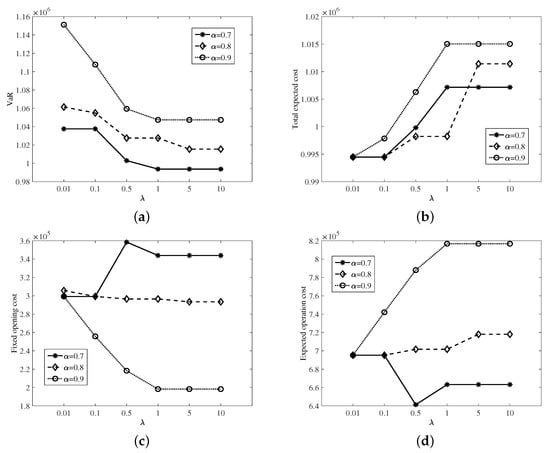
Figure 2.
Influences of risk parameters and on the results in the two-stage mean VaR stochastic programming model. (a) VaR versus . (b) Total expected cost versus . (c) Fixed opening cost versus . (d) Expected operation cost versus .

Table 4.
Detailed results of the mean VaR two-stage stochastic programming model under different risk parameters.
4.1.2. Sensitivity Analysis of Mean CVaR Two-Stage Stochastic Programming Model
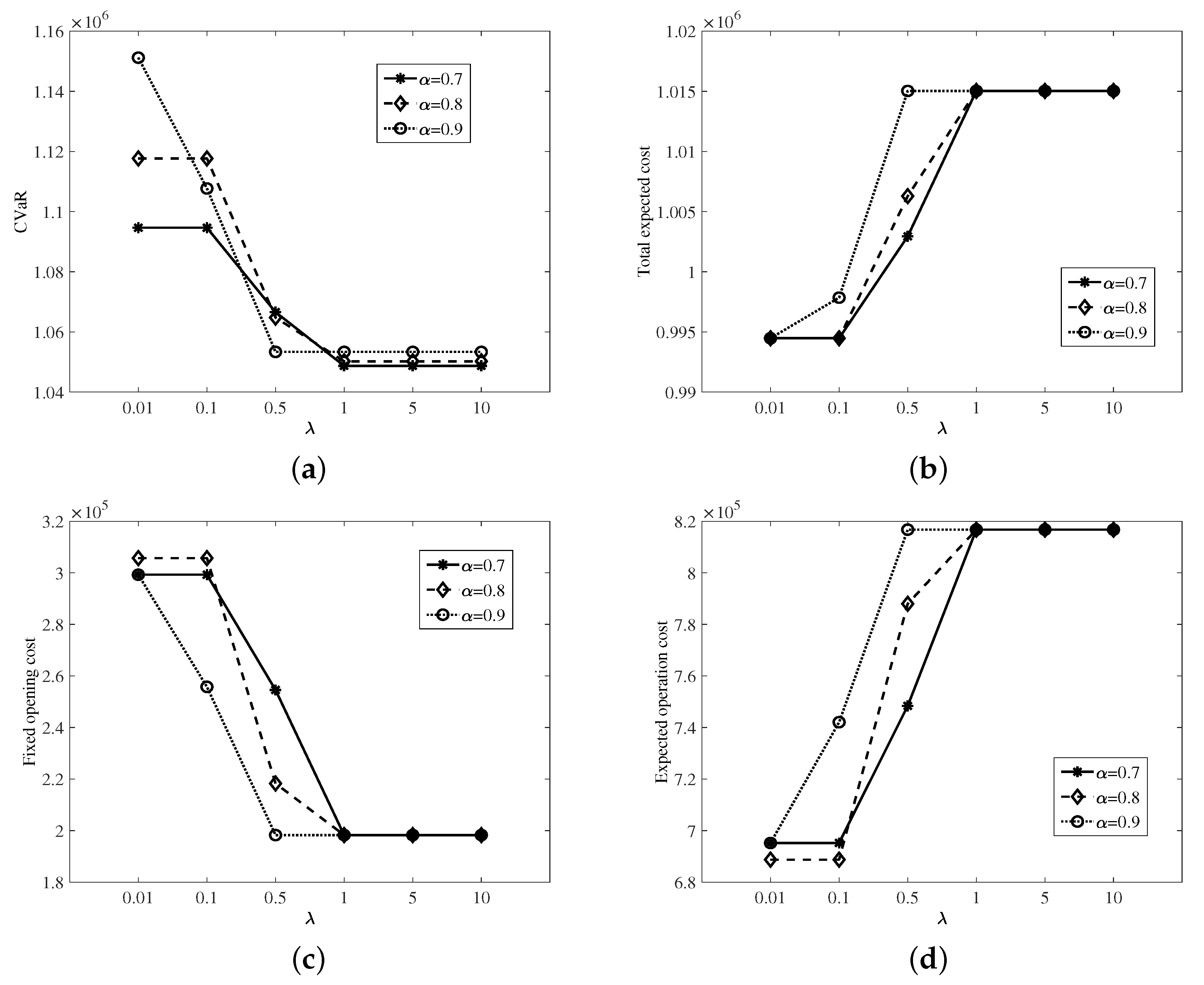
Figure 3 shows the sensitivity analysis on the CVaR, total expected cost, fixed opening cost, and expected operation cost of the mean CVaR two-stage stochastic programming model. In Figure 3a, it can be seen that, for a fixed , the value of CVaR decreases when increases. However, the total expected cost increases as increases, as shown in Figure 3b. Similar to the above mean VaR two-stage stochastic programming model, a larger represents an increase in the risk aversion level, which will lead to a lower CVaR value and a higher total expected cost. As shown in Figure 3c,d, for a fixed , the fixed opening cost may decrease but the expected operating cost may increase when the increases. Figure 3 also shows that CVaR, the total expected cost, fixed opening cost, and expected operation cost do not vary monotonically with . Table 5 shows the summary results of the mean CVaR two-stage stochastic programming model under different risk parameters.

Figure 3.
Influences of risk parameters on the results in the two-stage mean CVaR stochastic programming model. (a) CVaR versus . (b) Total expected cost versus . (c) Fixed opening cost versus . (d) Expected operation cost versus .

Table 5.
Detailed results of the mean CVaR two-stage stochastic programming model under different risk parameters.
4.2. Comparison with the Risk-Neutral Modeling Approach
In order to illustrate the significance of the risk-averse modeling approach, risk-averse two-stage stochastic programming models were solved under and , respectively. Moreover, the change in the total expected cost, the worst of the total cost, VaR, and CVaR were analyzed for different values of the risk parameters. Table 6 shows the total expected cost, the worst of the total cost, VaR, and CVaR of the total cost at confidence level for the optimal solution of the risk-neutral two-stage stochastic programming model (1)–(16).

Table 6.
Detailed results of the risk-neutral two-stage stochastic programming model.
4.2.1. Mean VaR Modeling Approach versus Risk-Neutral Modeling Approach
Table 7 shows the relative differences in the total expected cost, the worst of the total cost, VaR, and CVaR obtained by the mean VaR approach with respect to the corresponding values obtained by the risk-neutral approach. It can be seen that the mean VaR approach can obtain a smaller VaR than the risk-neutral approach. However, for the CVaR and the worst of the total cost, the mean VaR approach performs better than the risk-neutral approach only when the confidence level is large enough (. That is because when increases, CVaR and the worst of the total cost are close to VaR.

Table 7.
Mean VaR modeling approach versus risk-neutral modeling approach.
4.2.2. Mean CVaR Modeling Approach versus Risk-Neutral Modeling Approach
Table 8 presents the relative difference in the total expected cost, the worst of the total cost, VaR, and CVaR obtained by the mean CVaR approach with respect to the risk-neutral approach. It can be seen in Table 8 that CVaR, VaR, and the worst of the total cost obtained by the mean CVaR approach are all smaller than those obtained by the risk-neutral approach for different risk parameters. It is clear that, compared with the risk-neutral model, the mean CVaR approach performs more efficiently. It also reflects that CVaR, as a risk measure, can avoid risks more effectively than VaR.

Table 8.
Mean CVaR modeling approach versus the risk-neutral modeling approach.
4.3. Stochastic Measures
To illustrate the risk-averse two-stage stochastic programming approach to model the randomness, the stochastic measures were investigated. As discussed by [47], the stochastic measures for the proposed two risk-averse modeling approaches can be calculated as follows:
where is the optimal objective of the mean VaR two-stage stochastic programming (see Section 3.4.1); is the optimal objective of the mean CVaR two-stage stochastic programming (see Section 3.4.2); is the optimal total cost for scenario s, which is shown in Appendix A.
where is the operation cost in scenario s for the optimal solution of the expected value (EV) problem, in which the uncertain parameters are replaced by their expected value. The EV problem is formulated as shown in Appendix B.
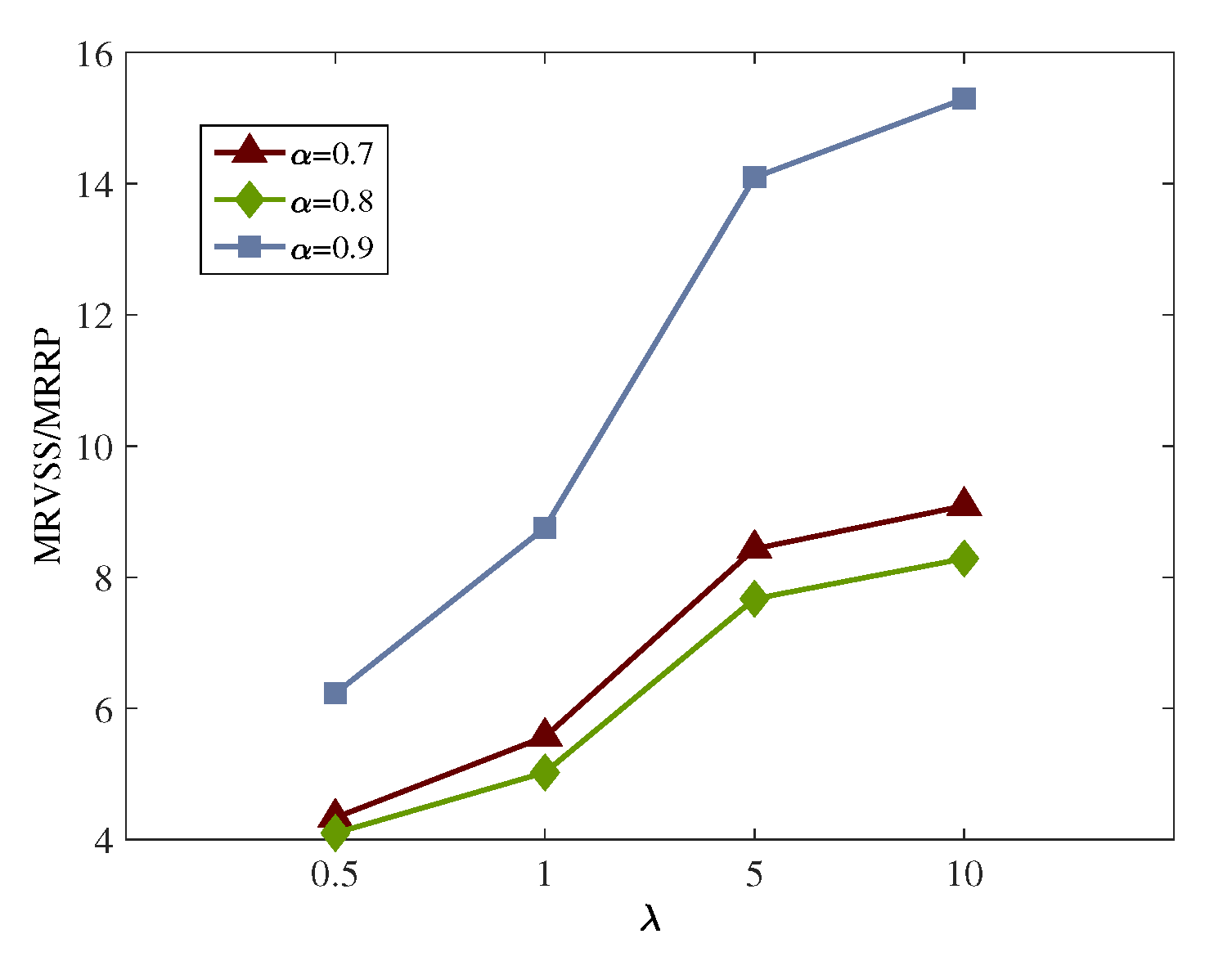
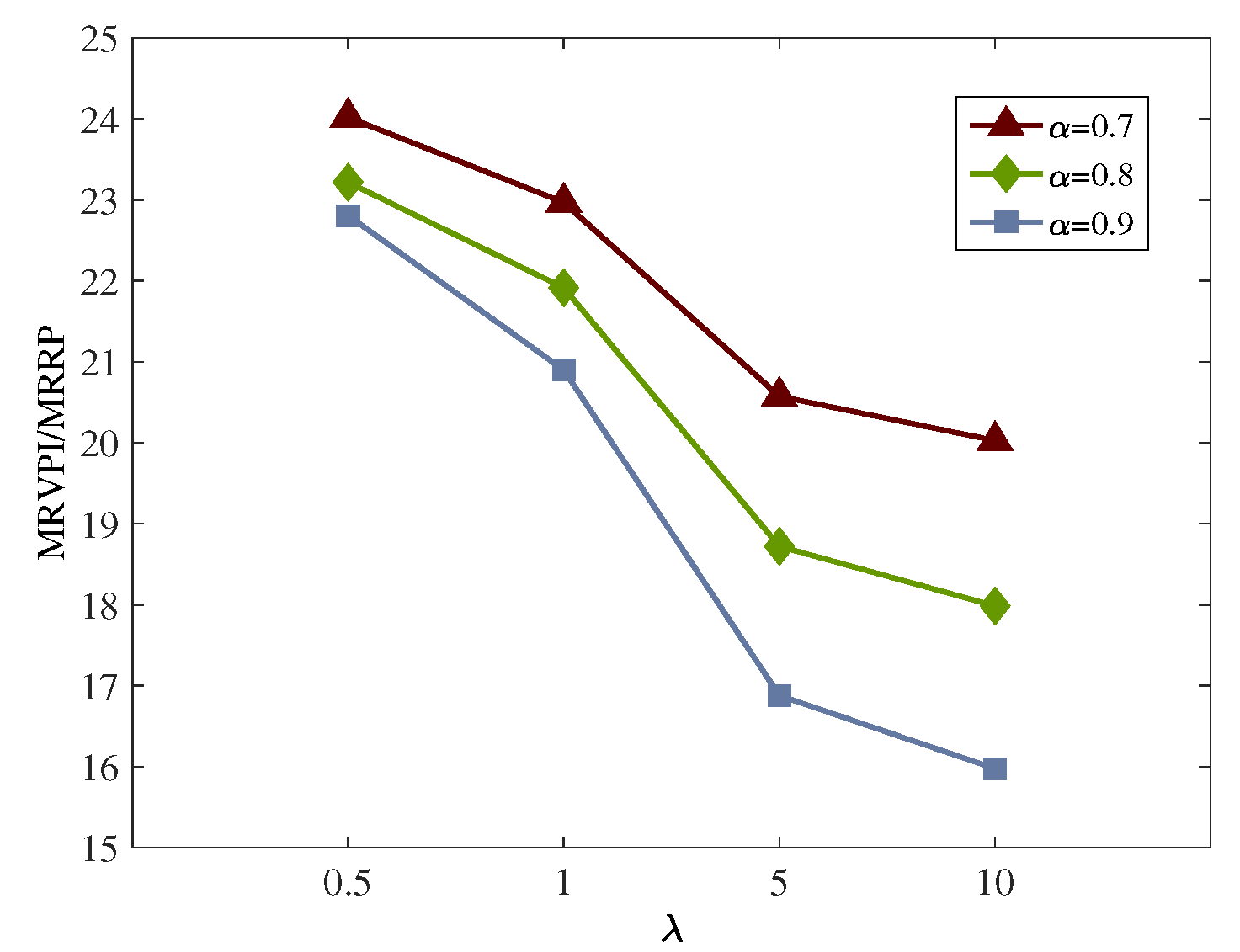
Figure 4 and Figure 5 illustrate the effects of risk parameters of the ratios and of the mean VaR modeling approach. As shown in Figure 4, for a fixed , the ratio increases when varies from 0.5 to 10. However, the ratio decreases as or increases, as seen in Figure 5. One can see in Figure 5 that the gap between the ratios under different tends to widen as increases. Table 9 shows the summary of the stochastic measures for the mean VaR modeling approach under different risk parameters, and .

Figure 4.
The value of under various and for the mean VaR modeling approach.

Figure 5.
The value of under various and for the mean VaR modeling approach.

Table 9.
Measures for the mean VaR modeling approach.
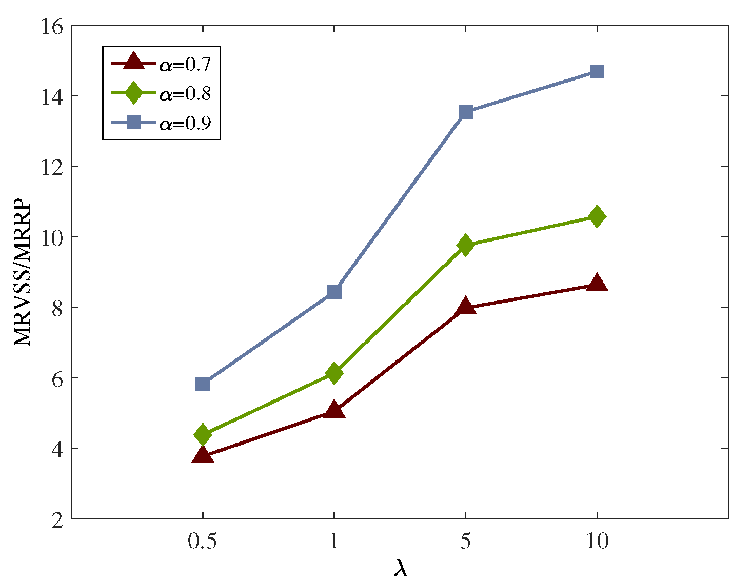
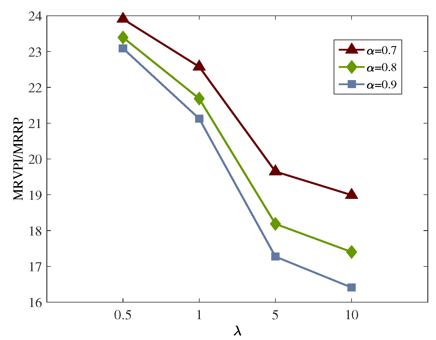
Figure 6 and Figure 7 illustrate the effects of risk parameters of the ratios and of the mean CVaR modeling approach. As seen in Figure 6, the ratio increases when varies from 0.5 to 10, and a larger value of can also lead to a higher value of . However, as shown in Figure 7, the ratio decreases as or increases. In Figure 7, one can see that the gap between the ratios under the different tends to widen when increases. Table 10 shows the summary of the stochastic measures for the mean CVaR modeling approach under different risk parameters and .
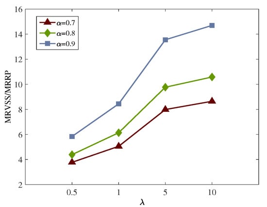
Figure 6.
The value of under various and for mean CVaR modeling approach.
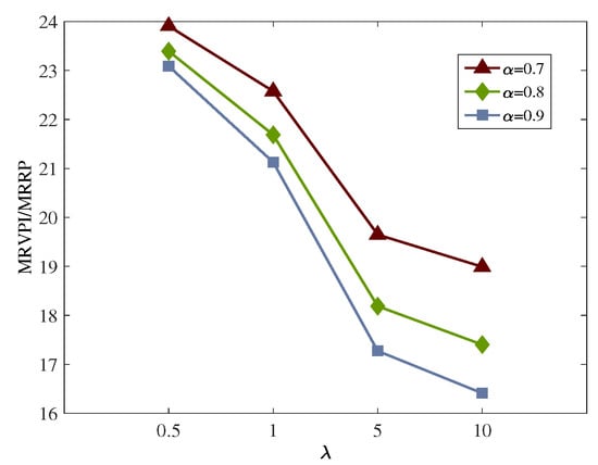
Figure 7.
The value of under various and for mean CVaR modeling approach.

Table 10.
Measures for the mean CVaR modeling approach.
5. Conclusions
A reverse logistics network design is important due to its impact on the efficiency of reverse logistics, which is receiving considerable attention from researches and practitioners. However, the existing studies have not considered uncertain disruptions and risk measures in the context of 3PL, simultaneously.
In this study, a risk-averse two-stage stochastic programming framework was proposed for designing a reverse logistics network under uncertain disruptions for 3PL. Two models were developed that incorporated VaR and CVaR into the mean risk objective function of risk-averse two-stage stochastic programming, respectively. Finally, sensitivity analyses of the risk parameters in the proposed two models were carried out. Moreover, the significance of the risk-averse modeling approach, with respect to the risk-neutral modeling approach, was verified. Stochastic measures were used to illustrate that the risk-averse two-stage stochastic programming approach could model the randomness efficiently.
This work can assist 3PL managers and deciders in designing an effective and reliable reverse logistics network with uncertain disruptions. The proposed models can be applied to other network design cases that consider uncertain disruptions or risk management.
Our study is not without limitations. There are some recommendations for future researches:
- In this paper, we considered single-type return products in the network. However, in many real cases, we have multiple-type return products, which can be a subject for future research.
- In this paper, the scenario-based stochastic programming method was applied to deal with disruption uncertainty. In future research, mixed uncertainty could be considered for this problem and there is a need to develop other approaches to confront (with uncertainty), such as fuzzy-stochastic programming.
- Because of the limitations of the solvers, we could not consider large problem sizes. Thus, developing a meta-heuristic algorithm for solving large-sized problems can be another interesting area for future research.
- Finally, some methods, such as Benders’ decomposition, can be employed to solve the proposed problem in future research.
Author Contributions
Conceptualization, R.L.; methodology, R.L.; software, R.L.; data curation, R.L.; writing—original draft preparation, R.L.; writing—review and editing, R.L. and X.C.; visualization, R.L. All authors have read and agreed to the published version of the manuscript.
Funding
This research was funded by the Natural Science Foundation of Liaoning Province of China (grant no. 20180550300), the Cooperation Innovation Plan of Yingkou for Enterprise and Doctor (grant no. 2022-13), and the Young Scientific and Technological Talents Project of the Educational Department of Liaoning Province, China (grant no. JQL202015407).
Institutional Review Board Statement
Not applicable.
Informed Consent Statement
Not applicable.
Data Availability Statement
The data presented in this study are available upon request from the corresponding author.
Acknowledgments
The authors would like to express our sincere thanks to the anonymous reviewers and editors for their time and patience devoted to the review of this paper.
Conflicts of Interest
The authors declare no conflict of interest.
Appendix A. The Optimal Total Cost of Each Scenario
The optimal total cost in scenario s can be calculated as follows:
s.t.
Appendix B. The EV Problem
In order to formulate the EV problem, the following decision variables are introduced:
| Quantity of products shipped from customer zone l to 3PL local collection center k | |
| Quantity of products shipped from 3PL local collection center k to 3PL centralized collection center j | |
| Quantity of products shipped from 3PL centralized collection center j to disposal center i | |
| Quantity of products shipped from 3PL centralized collection center j to plant m |
The EV problem is formulated as follows:
s.t.
The objective function (A4) is to minimize the total cost, including the fixed opening cost and optimal operation cost in the solution , where is the optimal value of the following problem:
s.t.
The objective function (A7) minimizes the operation cost. Equations (A8)–(A10) are the flow balance constraints for the 3PL local collection center and 3PL centralized collection centers. Constraint (A11) is related to limitations on the flow at customer zones. Equations (A12) and (A13) are the capacity constraints of the 3PL local collection center and 3PL centralized collection centers. Equations (A14) and (A15) are capacity constraints for disposal centers and plants, respectively. Equations (A16)–(A19) are related to the non-negative restrictions on decision variables.
References
- Tomislav, K. The concept of sustainable development: From its beginning to the contemporary issues. Zagreb Int. Rev. Econ. Bus. 2018, 21, 67–94. [Google Scholar]
- Manioudis, M.; Meramveliotakis, G. Broad strokes towards a grand theory in the analysis of sustainable development: A return to the classical political economy. New Political Econ. 2022, 27, 866–878. [Google Scholar] [CrossRef]
- Govindan, K.; Soleimani, H.; Kannan, D. Reverse logistics and closed-loop supply chain: A comprehensive review to explore the future. Eur. J. Oper. Res. 2015, 240, 603–626. [Google Scholar] [CrossRef]
- Kara, S.S.; Onut, S. A stochastic optimization approach for paper recycling reverse logistics network design under uncertainty. Int. J. Environ. Sci. Technol. 2010, 7, 717–730. [Google Scholar] [CrossRef]
- Ko, H.J.; Evans, G.W. A genetic algorithm-based heuristic for the dynamic integrated forward/reverse logistics network for 3PLs. Comput. Oper. Res. 2007, 34, 346–366. [Google Scholar] [CrossRef]
- Mahmoudzadeh, M.; Mansour, S.; Karimi, B. To develop a third-party reverse logistics network for end-of-life vehicles in Iran. Resour. Conserv. Recycl. 2013, 78, 1–14. [Google Scholar] [CrossRef]
- Hanafi, J.; Kara, S.; Kaebernick, H. Reverse logistics strategies for end-of-life products. Int. J. Logist. Manag. 2008, 19, 367–388. [Google Scholar] [CrossRef]
- Ivanov, D.; Dolgui, A.; Sokolov, B.; Ivanova, M. Literature review on disruption recovery in the supply chain. Int. J. Prod. Res. 2017, 55, 6158–6174. [Google Scholar] [CrossRef]
- Bugert, N.; Lasch, R. Supply chain disruption models: A critical review. Logist. Res. 2018, 11, 1–35. [Google Scholar]
- Snyder, L.V.; Atan, Z.; Peng, P.; Rong, Y.; Schmitt, A.J.; Sinsoysal, B. OR/MS models for supply chain disruptions: A review. IIE Trans. 2016, 48, 89–109. [Google Scholar] [CrossRef]
- Fleischmann, M.; Bloemhof-Ruwaard, J.M.; Dekker, R.; Van der Laan, E.; Van Nunen, J.A.; Van Wassenhove, L.N. Quantitative models for reverse logistics: A review. Eur. J. Oper. Res. 1997, 103, 1–17. [Google Scholar] [CrossRef]
- Mahaboob Sheriff, K.M.; Gunasekaran, A.; Nachiappan, S. Reverse logistics network design: A review on strategic perspective. Int. J. Logist. Syst. Manag. 2012, 12, 171–194. [Google Scholar]
- Suyabatmaz, A.Ç.; Altekin, F.T.; Şahin, G. Hybrid simulation-analytical modeling approaches for the reverse logistics network design of a third-party logistics provider. Comput. Ind. Eng. 2014, 70, 74–89. [Google Scholar] [CrossRef]
- Kannan, D.; Garg, K.; Jha, P.C.; Diabat, A. Integrating disassembly line balancing in the planning of a reverse logistics network from the perspective of a third party provider. Ann. Oper. Res. 2017, 253, 353–376. [Google Scholar] [CrossRef]
- Eskandarpour, M.; Nikbakhsh, E.; Zegordi, S.H. Variable neighborhood search for the bi-objective post-sales network design problem: A fitness landscape analysis approach. Comput. Oper. Res. 2014, 52, 300–314. [Google Scholar] [CrossRef]
- Min, H.; Ko, H.J. The dynamic design of a reverse logistics network from the perspective of third-party logistics service providers. Int. J. Prod. Econ. 2008, 113, 176–192. [Google Scholar] [CrossRef]
- Du, F.; Evans, G.W. A bi-objective reverse logistics network analysis for post-sale service. Comput. Oper. Res. 2008, 35, 2617–2634. [Google Scholar] [CrossRef]
- Lee, D.H.; Bian, W.; Dong, M. Multiobjective model and solution method for integrated forward and reverse logistics network design for third-party logistics providers. Transp. Res. Rec. 2007, 2032, 43–52. [Google Scholar] [CrossRef]
- Lee, D.H.; Bian, W.; Dong, M. Multiproduct distribution network design of third-party logistics providers with reverse logistics operations. Transp. Res. Rec. 2007, 2008, 26–33. [Google Scholar] [CrossRef]
- Lee, H.; Zhang, T.; Boile, M.; Theofanis, S.; Choo, S. Designing an integrated logistics network in a supply chain system. KSCE J. Civ. Eng. 2013, 17, 806–814. [Google Scholar] [CrossRef]
- Ghafarimoghadam, A.; Ghayebloo, S.; Pishvaee, M.S. A fuzzy-budgeted robust optimization model for joint network design-pricing problem in a forward-reverse supply chain: The viewpoint of third-party logistics. Comput. Appl. Math. 2019, 38, 1–29. [Google Scholar] [CrossRef]
- Ayvaz, B.; Bolat, B.; Aydın, N. Stochastic reverse logistics network design for waste of electrical and electronic equipment. Resour. Conserv. Recycl. 2015, 104, 391–404. [Google Scholar] [CrossRef]
- Trochu, J.; Chaabane, A.; Ouhimmou, M. A two-stage stochastic optimization model for the reverse logistics network design under dynamic suppliers’ locations. Waste Manag. 2019, 95, 569–583. [Google Scholar] [CrossRef] [PubMed]
- Yu, H.; Solvang, W.D. A carbon-constrained stochastic optimization model with augmented multi-criteria scenario-based risk-averse solution for the reverse logistics network design under uncertainty. J. Clean. Prod. 2017, 164, 1248–1267. [Google Scholar] [CrossRef]
- Fonseca, M.C.; García-Sánchez, Á.; Ortega-Mier, M.; Saldanha-da-Gama, F. A stochastic bi-objective location model for strategic reverse logistics. Top 2010, 18, 158–184. [Google Scholar] [CrossRef]
- Yu, H.; Solvang, W.D. Incorporating flexible capacity in the planning of a multi-product multi-echelon sustainable reverse logistics network under uncertainty. J. Clean. Prod. 2018, 198, 285–303. [Google Scholar] [CrossRef]
- Roudbari, E.S.; Ghomi, S.F.; Sajadieh, M.S. Reverse logistics network design for product reuse, remanufacturing, recycling and refurbishing under uncertainty. J. Manuf. Syst. 2021, 60, 473–486. [Google Scholar] [CrossRef]
- Fattahi, M.; Govindan, K. Integrated forward/reverse logistics network design under uncertainty with pricing for collection of used products. Ann. Oper. Res. 2017, 253, 193–225. [Google Scholar] [CrossRef]
- Pishvaee, M.S.; Jolai, F.; Razmi, J. A stochastic optimization model for integrated forward/reverse logistics network design. J. Manuf. Syst. 2009, 28, 107–114. [Google Scholar] [CrossRef]
- Vahdat, V.; Vahdatzad, M.A. Accelerated Benders’ decomposition for integrated forward/reverse logistics network design under uncertainty. Logistics 2017, 1, 11. [Google Scholar] [CrossRef]
- Sugimura, Y.; Murakami, S. Designing a Resilient International Reverse Logistics Network for Material Cycles: A Japanese Case Study. Resour. Conserv. Recycl. 2021, 170, 105603. [Google Scholar] [CrossRef]
- Govindan, K.; Gholizadeh, H. Robust network design for sustainable-resilient reverse logistics network using big data: A case study of end-of-life vehicles. Transp. Res. Part Logist. Transp. Rev. 2021, 149, 102279. [Google Scholar] [CrossRef]
- Ghomi-Avili, M.; Khosrojerdi, A.; Tavakkoli-Moghaddam, R. A multi-objective model for the closed-loop supply chain network design with a price-dependent demand, shortage and disruption. J. Intell. Fuzzy Syst. 2019, 36, 5261–5272. [Google Scholar] [CrossRef]
- Yavari, M.; Zaker, H. An integrated two-layer network model for designing a resilient green-closed loop supply chain of perishable products under disruption. J. Clean. Prod. 2019, 230, 198–218. [Google Scholar] [CrossRef]
- Yavari, M.; Zaker, H. Designing a resilient-green closed loop supply chain network for perishable products by considering disruption in both supply chain and power networks. Comput. Chem. Eng. 2020, 134, 106680. [Google Scholar] [CrossRef]
- Hatefi, S.M.; Jolai, F. Reliable forward-reverse logistics network design under partial and complete facility disruptions. Int. J. Logist. Syst. Manag. 2015, 20, 370–394. [Google Scholar] [CrossRef]
- Torabi, S.; Namdar, J.; Hatefi, S.; Jolai, F. An enhanced possibilistic programming approach for reliable closed-loop supply chain network design. Int. J. Prod. Res. 2016, 54, 1358–1387. [Google Scholar] [CrossRef]
- Jabbarzadeh, A.; Haughton, M.; Khosrojerdi, A. Closed-loop supply chain network design under disruption risks: A robust approach with real world application. Comput. Ind. Eng. 2018, 116, 178–191. [Google Scholar] [CrossRef]
- Hatefi, S.; Jolai, F. Robust and reliable forward–reverse logistics network design under demand uncertainty and facility disruptions. Appl. Math. Model. 2014, 38, 2630–2647. [Google Scholar] [CrossRef]
- Fazli-Khalaf, M.; Mirzazadeh, A.; Pishvaee, M.S. A robust fuzzy stochastic programming model for the design of a reliable green closed-loop supply chain network. Hum. Ecol. Risk Assessment Int. J. 2017, 23, 2119–2149. [Google Scholar] [CrossRef]
- Rahimi, M.; Ghezavati, V. Sustainable multi-period reverse logistics network design and planning under uncertainty utilizing conditional value at risk (CVaR) for recycling construction and demolition waste. J. Clean. Prod. 2018, 172, 1567–1581. [Google Scholar] [CrossRef]
- Soleimani, H.; Govindan, K. Reverse logistics network design and planning utilizing conditional value at risk. Eur. J. Oper. Res. 2014, 237, 487–497. [Google Scholar] [CrossRef]
- Ma, L.; Liu, Y.; Liu, Y. Distributionally robust design for bicycle-sharing closed-loop supply chain network under risk-averse criterion. J. Clean. Prod. 2020, 246, 118967. [Google Scholar] [CrossRef]
- Soleimani, H.; Seyyed-Esfahani, M.; Kannan, G. Incorporating risk measures in closed-loop supply chain network design. Int. J. Prod. Res. 2014, 52, 1843–1867. [Google Scholar] [CrossRef]
- Ramezani, M.; Bashiri, M.; Tavakkoli-Moghaddam, R. A new multi-objective stochastic model for a forward/reverse logistic network design with responsiveness and quality level. Appl. Math. Model. 2013, 37, 328–344. [Google Scholar] [CrossRef]
- Fard, A.F.; Gholian-Jouybari, F.; Paydar, M.M.; Hajiaghaei-Keshteli, M. A bi-objective stochastic closed-loop supply chain network design problem considering downside risk. Ind. Eng. Manag. Syst. 2017, 16, 342–362. [Google Scholar]
- Noyan, N. Risk-averse two-stage stochastic programming with an application to disaster management. Comput. Oper. Res. 2012, 39, 541–559. [Google Scholar] [CrossRef]
- Rockafellar, R.T.; Uryasev, S. Conditional value-at-risk for general loss distributions. J. Bank. Financ. 2002, 26, 1443–1471. [Google Scholar] [CrossRef]
Publisher’s Note: MDPI stays neutral with regard to jurisdictional claims in published maps and institutional affiliations. |
© 2022 by the authors. Licensee MDPI, Basel, Switzerland. This article is an open access article distributed under the terms and conditions of the Creative Commons Attribution (CC BY) license (https://creativecommons.org/licenses/by/4.0/).


