Article

Spatial Distribution of Leisure Agriculture in Xinjiang and Its Influencing Factors Based on Geographically Weighted Regression

1
College of Geography and Remote Sensing Sciences, Xinjiang University, Urumqi 830046, China
2
Key Laboratory of Wisdom City and Environment Modeling of Higher Education Institute, Urumqi 830046, China
3
College of Resources and Environmental Engineering, Ludong University, Yantai 264025, China
4
Institute of Water Science, Beijing Normal University, Beijing 100875, China
*
Author to whom correspondence should be addressed.
Sustainability 2022, 14(22), 15002; https://doi.org/10.3390/su142215002
Submission received: 3 August 2022 / Revised: 30 October 2022 / Accepted: 8 November 2022 / Published: 13 November 2022
(This article belongs to the Section Sustainable Agriculture)

Abstract

:
As a new industry in modern agriculture, leisure agriculture has a strong correlation with rural tourism, and provides rural areas with positive prospects for sustainable development. However, leisure agriculture tends to include a number of bottlenecks. In this study, we investigated the spatial distribution of leisure agriculture in Xinjiang, and the factors that affect it. Kernel density analysis, the nearest-neighbor index, and the geographic concentration index were used to analyze the distribution characteristics of leisure agriculture. Following the conclusion of the ordinary least squares tests, geographically weighted regression (GWR) was conducted to explore the factors affecting spatial distribution. The findings were as follows: (1) The spatial distribution of leisure agriculture in Xinjiang is uneven, and is concentrated in the northern and southern parts of the Tianshan Mountains in western Xinjiang. (2) In terms of the distribution density, there are four high-concentration centers (Bosten Lake, Hami, and the east and west sides of the Ili River Valley) and one subconcentration center (spreading outward from Urumqi). (3) Population, transportation, tourism resources, urban factors, and rainfall, all had significant effects on the distribution of leisure agriculture. These factors had positive and negative effects on the distribution of leisure agriculture, forming high- and low-value areas in space. (4) The leisure agricultural sector responded in varying degrees to the different factors, with large internal variability. Rainfall and population had greater differential effects on the spatial distribution of leisure agriculture compared to transportation, tourism resources, and urban factors, and there were significant two-way effects. Transportation, urban factors, and tourism resources all had consistent, predominantly positive, effects on the distribution of leisure agriculture.

1. Introduction

1.1. Leisure Agriculture and Sustainability

Harnessing the potential of sustainable industries to promote underdeveloped industrial linkages is important for developing countries [1]. One way to achieve this is through tourism. Tourism is also a major contributor to carbon emissions [2]. Although tourism depends on other industries to carry out its activities, it is often weakly integrated with other industries [3]. In less developed areas, the combination of rurality and tourism can have important benefits for sustainability [4]. For example, rural development projects in Europe have been shown to help improve the welfare of rural populations and reduce rural–urban imbalances [5]. Accordingly, governments have increasingly recognized the potential of forming synergistic relationships between tourism and agriculture [6]. Through policy interventions, rural tourism can contribute to economic growth in rural areas and poor or marginalized sectors [7]. From 2009 to 2019, research on rural tourism focused primarily on sustainable development [8], which is a key topic in current research [9]. In addition, some studies have reported significant differences in the carbon emissions per capita of different types of tourism [10].
Leisure agriculture is a light form of agricultural production, related to travel and leisure, and has become a typical model of rural tourism. The concept originated in the 1830s, during a time of rapid urbanization and population explosion. In this period, people sought leisure in the countryside in order to relieve themselves of urban pressures. Leisure agriculture first appeared in Austria and other European countries [11]. In the context of rural revitalization, leisure agriculture is related to rural industry [12], village systems, urban–rural integration, and tourism planning [13,14]. Leisure agriculture is an important means of solving the contradiction between economic development and ecological protection, and of promoting sustainable social development [15]. In the context of the COVID-19 pandemic, there has been an increase in short trips [16]. Under commercial marketing, tourism operators should observe the demand preferences of consumers [17]. These travelers have developed a strong interest in leisure agriculture [18]. Leisure agriculture has been shown to be profitable [19] and is now a key sector in the context of sustainable development [20]. However, its ability to maintain stable employment and profits depends on the stability of tourism activities throughout the year [21]. Previous research on leisure agriculture has focused on three main aspects: (1) the industrialization of leisure agriculture, leading and trailing industries, economic structural optimization, and environmental aspects [22]; (2) business models for leisure agriculture in different regions, focusing on industry operations and the factors affecting them [23,24]; and (3) the consumption status and guest market of leisure agriculture from a microeconomic perspective [25].

1.2. Geographically Weighted Regression

Recent research in spatial statistics and related fields has focused on the heterogeneity, or non-smoothness, of spatial data relationships, proposing techniques based on local spatial statistical analysis [26]. In this regard, many studies have used geographically weighted regression (GWR), which quantifies the heterogeneity, or non-smoothness, of spatial data relationships through local weighted regression analysis of the location, producing parameter estimation results that vary across different spatial locations. Zhou et al. [27] used GWR to evaluate the effects of different factors on haze pollution in 285 cities in China. In addition, Gu [28] predicted a surge in travel demand after COVID-19. In a related study, Liu et al. used susceptible exposed-infected-recovered-dead (SEIRD) and Long Short-Term Memory (LSTM) models to predict the epidemic situation in Wuhan and found that, after accounting for the effect of the geographical differences, the GWR results had the best fit [29,30]. Moreover, they found that GWR could identify the spatial non-stationarity of the factors affecting dengue virus transmission in Malaysia. As a spatial regression model that considers the geographic location [31], GWR has been shown to outperform traditional linear regression models in studying the spatial heterogeneity of effects [32,33]. Taking certain Italian provinces as the study area, Casolani et al. [34] used GWR to construct a model that included agricultural water storage and certain climatic variables. Other researchers have constructed models using topography, urbanization [35], and economic development, among other factors, as variables to explore environmental effect mechanisms. According to the above-mentioned studies, the GWR model has been used in different scientific fields. This study uses the same research methodology to assess the mechanisms of influence of different factors on the distribution of leisure agriculture.
As a sustainable activity, leisure agriculture can have benefits for ecology, production, and life [36]. Xinjiang is located in an arid and semi-arid region in western China. It has a very different energy consumption structure compared with other parts of China, and its population consumption structure affects its carbon emissions to a certain extent [37]. The sustainability of leisure agriculture should be adapted to local conditions, unified layout and ecological cycle. Selecting agricultural crops with high carbon absorption levels and compatibility with the natural conditions of the region will allow the realization of the economic benefits of agricultural production and tourism development, while maximizing the carbon sink potential of the crops to obtain good economic and ecological benefits [38]. In this study, the spatial distribution and influencing factors of leisure agriculture in Xinjiang were investigated to promote its environmentally sustainable development [39] and provide suggestions for tourism development and poverty alleviation [40].

2. Materials and Methods

2.1. Overview of the Study Area

Xinjiang (Figure 1) (73°40′–96°18′ E, 34°25′–48°10′ N) is located in the arid and semiarid region of northwest China, occupying approximately one-sixth of China’s total area. Its topography is distributed, north to south, in the Altay Mountains, Junggar Basin, Tianshan Mountains, Tarim Basin, and the Kunlun Mountains, with oases scattered in between these features. The climate of Xinjiang is temperate continental, with basins and mountain ranges distributed throughout the area [41]. With a GDP of RMB 1598.365 billion in 2021, Xinjiang is an important economic corridor between China and Central Asia, West Asia, and Europe [42]. The entire territory of Xinjiang was taken as the study area of this paper, including all of the autonomous prefectures, prefecture-level cities and regions in the entire territory of Xinjiang.

2.2. Data Sources

The Digital Elevation Model (DEM) is a powerful data to simulate the impact of topography. In addition, other data for simulating natural factors and socio-economic impacts, such as average annual rainfall grid data (30 m), population distribution grid data (30 m), and gross domestic product (GDP), need to be considered. Road traffic vector data, including railroads, highways, national highways and urban trunk roads, as well as town distribution vectors, including prefecture-level cities and counties, are derived from the National Basic Geographic Information System (NBGIS). Using the AMAP development platform and Bigemap map downloader, the names and geographic information coordinates of leisure agriculture points in Xinjiang were obtained with the keywords of farmhouse, leisure orchard, leisure farm and leisure village. The data from the official website of Xinjiang Department of Culture and Tourism were checked and filtered, and, finally, the distribution data of leisure agriculture points in Xinjiang were compiled (Table 1).

2.3. Methods

2.3.1. Nearest-Neighbor Index

The nearest-neighbor index [43] can be used to describe the spatial proximity of point data. The type of spatial distribution of the elements is judged according to the magnitude of the calculated index:
R = r 1 r E ,
r E = 1 2 n / A ,
where R is the nearest-neighbor index, r1 is the nearest-neighbor distance, rE is the theoretical nearest-neighbor distance, n is the number of leisure agriculture points, and A is the area of the study area. When R = 1, the distribution of the leisure agriculture in Xinjiang is random; when R > 1, it is uniform; and when R < 1, it is agglomerative.

2.3.2. Geographic Concentration Index

This index [33] is used to study the degree of the spatial concentration of point-like elements. Its value interval is [0, 100]. When the value is closer to 100, the degree of the concentration of the elements is higher; and when the value is closer to 0, the degree of concentration of the elements is lower. The formula is
G = i = 1 n P i Q 2 × 100 ,
where G is the geographic concentration index, Pi is the number of leisure agriculture points in the ith prefecture and city, n is the number of prefectures and cities, and Q is the total number of leisure agriculture points. The value of G is within the range of [0, 100]. The larger the value, the more concentrated the distribution; and the smaller the value, the more dispersed the distribution.

2.3.3. Imbalance Index

The imbalance index [44] is used to describe the spatial equilibrium of elements and takes a value within the range [0, 1]. The closer the value to 1, the more unbalanced the distribution; and 0 indicates the average distribution of the elements in space:
S = i = 1 n Y i 50 ( n + 1 ) 100 × n 50 ( n + 1 ) ,
where S is the imbalance index, n is the number of prefectures and cities, and Yi is the cumulative percentage of the number of leisure agriculture points in each prefecture and city in the ith location, after ranking from the largest proportion to the smallest. The value of S ranges from 0 to 1. The larger the value, the more unbalanced the distribution. If S = 0, the distribution is even within each prefecture and city; and if S = 1, everything is concentrated in one prefecture or city.

2.3.4. Kernel Density Analysis

When analyzing the spatial clustering characteristics of point elements, kernel density analysis [45] can reflect the relative concentration of the spatial distribution of the elements [46]. It can be used to study the spatial distribution of the data from the data themselves. The larger the kernel density value, the denser the distribution of data. The formula is as follows:
f h ( x ) = 1 n h i = 1 n x x i h ,
where fh(x) is the kernel density function, and xxi is the distance from x to xi. h is the width and is greater than 0. A larger value of fh(x) indicates a denser distribution.

2.3.5. Standard Deviation Ellipses

Standard deviation ellipses [47,48] are used to identify the direction of data distributions, trends, distribution characteristics, and potential correlations with specific elements. The semi-major axis of the ellipse indicates the direction of the data distribution, and the semi-minor axis indicates the range of the data distribution. The greater the flatness, the more obvious the directionality of the data distribution. It is expressed as follows:
Average center:
X ¯ w = i = 1 n w i x i / i = 1 n w i , Y ¯ w = i = 1 n w i y i / i = 1 n w i ,
Elliptical azimuth:
tan θ = ( A + B ) / C ,
A = ( i = 1 n w i 2 x ˜ i 2 i = 1 n w i 2 y ˜ i 2 ) ,
B = ( i = 1 n w i 2 x ˜ i 2 i = 1 n y ˜ i 2 ) 2 + 4 i = 1 n w i 2 x ˜ i 2 y ˜ i 2 ,
C = 2 i = 1 n w i 2 x ˜ i y ˜ i ,
x-axis standard deviation:
ρ x = i = 1 n ( w i x ˜ i cos θ - w i y ˜ i sin θ ) 2 / i = 1 n w i 2 ,
y-axis standard deviation:
ρ y = i = 1 n ( w i x ˜ i sin θ - w i y ˜ i cos θ ) 2 / i = 1 n w i 2 ,
In Equations (6)–(12), ( X ¯ w, Y ¯ w) is the mean center of the spatial element, wi is the weight at spatial element i, (xi, yi) is the spatial coordinate, and ρx and ρy denote the standard deviation of the X and Y axes, respectively. θ is the azimuth of the ellipse, and xi and yi are the deviations of the spatial coordinate of the study object from the mean center coordinate.

2.3.6. Geographically Weighted Regression

GWR is an extension of linear regression [36,49]. The main difference is that the spatial characteristics of the variables are incorporated into the model to study the spatial non-stationarity among the variables from a local perspective. Its regression coefficient βi is continuously changes with the spatial location i of the element, thus reflecting the influence of the independent variable on the dependent variable with the spatial location:
y i = β 0 ( u i , v i ) + k = 1 n β k ( u i , v i ) x i k + ε i
where (ui, vi) is the geographical coordinates of the ith sample spatial unit, βk (ui, vi) is the kth regression coefficient of sample spatial unit i, yi is the number of leisure agriculture points in the ith sample spatial unit, xik is the observed value of the kth influencing factor at spatial unit (ui, vi), k denotes the factors that may affect the spatial distribution of the leisure agriculture (e.g., rainfall, tourism resources, population, city, and transportation), and n is the number of influencing factors. In addition, εi is the residual term and obeys a normal distribution. The smaller the residual, the better the fit of the regression equation.

2.3.7. Lorenz Curve

The Lorenz curve [50] is a method of measuring fairness, proposed by the American statistician Lorenz, which can visually analyze the fairness of social distribution. The basic principle is to divide income into a number of classes and arrange them, cumulatively, from the smallest to the largest percentage on the vertical axis, and connect the points with the corresponding cumulative percentage of the population on the horizontal axis to obtain the Lorenz curve [51]. Originally used to measure the wealth gap of a country, it is now widely used to compare the equilibrium of various types of resource allocation. In this paper, the Lorenz curve is plotted by the cumulative percentage of data points of leisure agriculture in different regions. The flatter the arc of the Lorenz curve, the closer it is to the absolute mean, and the better the equilibrium is.

3. Analysis and Results

3.1. Analysis of Spatial Distribution

3.1.1. Type of Spatial Distribution

Most of the leisure agriculture sites in Xinjiang are located in the area north of the Tianshan Mountains (Figure 2). The area south of the Tianshan Mountains forms a loose distribution in a ring around the Taklamakan Desert. At the time of this study, there were 1150 leisure agriculture sites in the northern border area, occupying nearly 66% of Xinjiang. Among them, because of unique soil and water resources, in the Ili Kazakh Autonomous Prefecture (this statistic only includes the counties and cities directly under the Ili Prefecture; hereinafter referred to as Ili), the leisure agriculture was distributed in approximately 405 sites, accounting for approximately 28% of all of Xinjiang, and representing the most distributed leisure agriculture in Xinjiang. The Bayingoleng Mongol Autonomous Prefecture (hereinafter referred to as, Bazhou) had the second most abundant leisure agriculture, with 304 sites, making it the most densely distributed area in southern Xinjiang. These sites were predominantly clustered in the southern foothills of the Tianshan Mountains and around Bosten Lake. The southern Bazhou and Hotan areas had sparsely distributed leisure agriculture sites, owing to their extensive deserts, sparse populations, and lack of water resources. Areas such as Aksu and Kashgar were important tourist areas in western Xinjiang, where the distribution of oases and tourism development have led to the development of leisure agriculture.
The analysis (Table 2) revealed that the average observation distance of leisure agriculture in Xinjiang was r1 = 2.8 km, the theoretical closest distance rE = 15.5 km, and the closest proximity index was R = 0.179 (<1). This indicates that the leisure agriculture points exhibited a cluster distribution type in terms of their spatial distribution.
The standard deviation ellipse was used to determine the agglomerations of the leisure agriculture point distribution. The standard deviation ellipse was drawn using the 1_STANDARD_DEVIATION model (Figure 2), covering approximately 68% of the leisure agriculture data points. The long axis of the oval shape in Figure 2 shows that the main distribution of the leisure agriculture in Xinjiang was in the northeast–southwest direction and was primarily concentrated in central and western Xinjiang. The short axis illustrates the breadth of the distribution of the leisure agriculture sites. The short axis extends from the north-western part of Bazhou to the national border of Tacheng, with an elliptical flatness of 0.55 (Table 3). The leisure agriculture sites were concentrated on either side of the Tianshan Mountains in the west.

3.1.2. Equilibrium of Spatial Distribution

The geographic concentration index (Table 2) was calculated using the leisure agriculture data points to obtain G = 37.6226. Assuming that 1745 leisure agriculture sites were distributed among the 14 prefectures and cities in Xinjiang, then, on average, there are 124.5 sites in each prefecture. The geographic concentration index was G0 = 26.7261, and G > G0, indicating that the distribution of the leisure agriculture sites was more concentrated at the prefectures and cities scale, with places such as Ili and Hami in the northern region containing >150 sites, while the Kizilsu Kirgiz Autonomous Prefecture in the southern region (hereinafter referred to as, Kezhou) in southern Xinjiang only contained 20 sites. The imbalance index (Table 2) was used to quantify the degree of imbalance of the distribution of the leisure agriculture across the territory, and the state of imbalance was calculated to be S = 0.48 (<1). A Lorenz curve (Figure 3) was plotted, exhibiting an upward convex trend, with Ili and Bazhou alone accounting for almost 50% of the distribution of the leisure agriculture in the entire territory. This verified the unevenness of the distribution. The two main reasons for the above-mentioned phenomenon are as follows. (1) Geographical location: both places are located around the Tianshan Mountains, to the north and south, with the topography of Ili opening to the west. This is conducive to receiving the prevailing westerly winds from the Atlantic Ocean and reflects unique natural conditions. (2) Area: Xinjiang is a vast area, and short-distance rural leisure agriculture tourism has more advantages than long-distance, for example, time-consuming travel.

3.1.3. Spatial Distribution Density

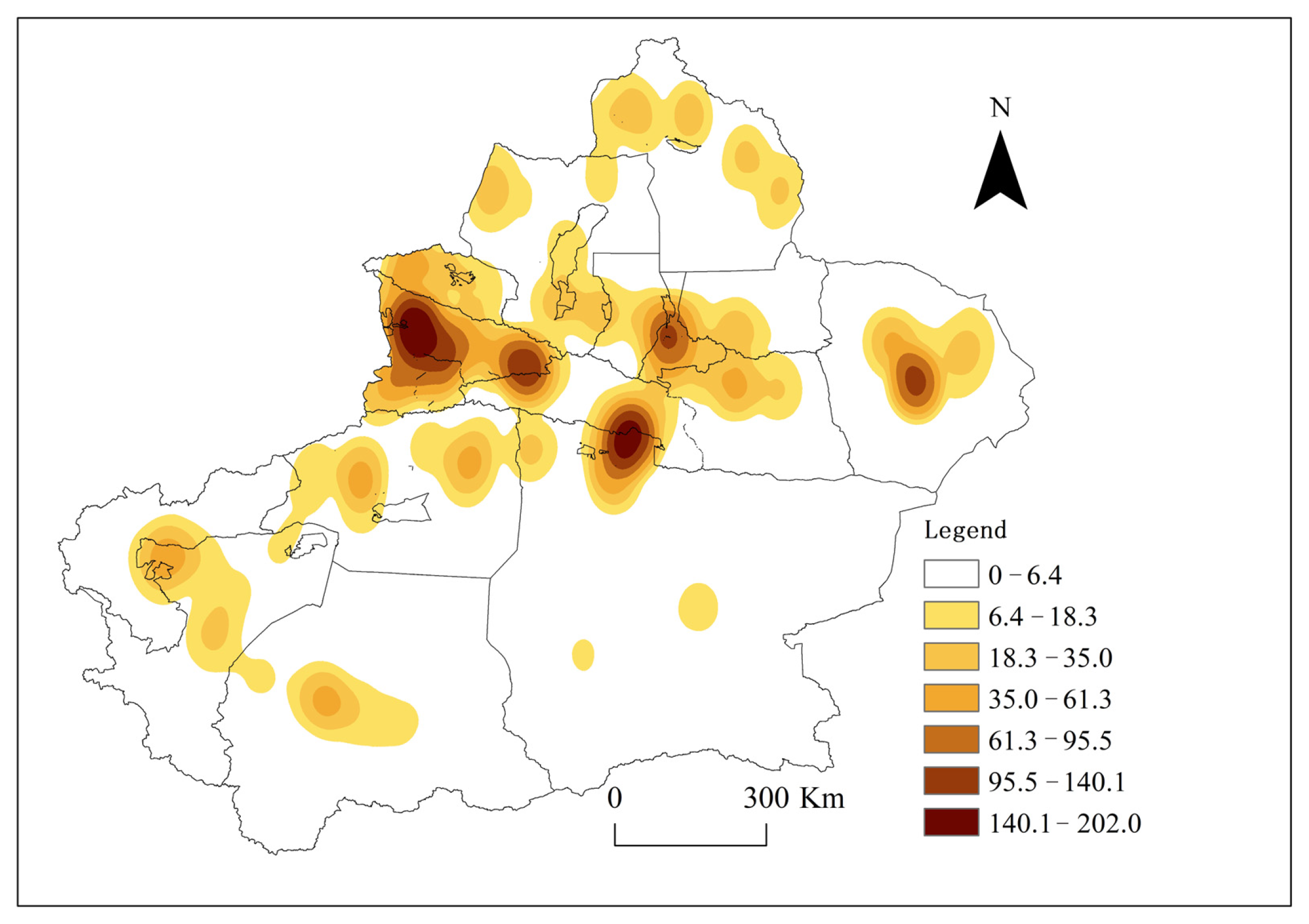
Kernel density analysis of the leisure agriculture data points in the entire territory (Figure 4) revealed that four high-concentration centers and one secondary concentration center had formed in the territory. The four high-concentration centers were located on the east and west sides of the Ili Valley, around Bosten Lake, and in Hami. All four centers were distributed on the north and south sides of the Tianshan Mountains. The high-density area on the west side of the Ili Valley radiated in all directions, with Yining City as the core. On the east side, the Narathi Grassland Scenic Area was the center. Korla City formed a high-concentration area, due to the tourist attractions of Bosten Lake. Hami is an important melon-producing area in China, supplying Hami melons and other agricultural products to the entire country. Leisure agriculture, primarily picking gardens, resulted in the high-concentration area in Hami, accounting for 161 sites. Urumqi was the only subcollection center. It was the core city of the Tianshan North Slope City Cluster, and it drove the development of leisure agriculture in the surrounding area to meet the daily short-distance recreational activity needs of the urban population.

3.2. Factor Selection

Natural factors: Xinjiang has a dry climate and little rainfall, as well as an interspersed distribution of high mountain basins and widespread desert. Thus, the topography and rainfall are important factors that may affect the distribution of leisure agriculture.
Social factors: With the development of sustainable tourism in China, leisure agriculture has become a tourism hotspot in Xinjiang and has attracted local residents and tourists. Any form of tourism must consider the relationship between the source markets, source channels, and tourism resources.
Based on the above-mentioned factors, seven variables that may affect the distribution of leisure agriculture were selected for GWR: population, economy, transportation, town distribution, tourism resource, average annual rainfall, and topographic factors. Then, based on this, the factors affecting the distribution of the leisure agriculture were explored. Table 4 presents the analysis indexes and calculation methods for each factor.

3.3. Model Construction

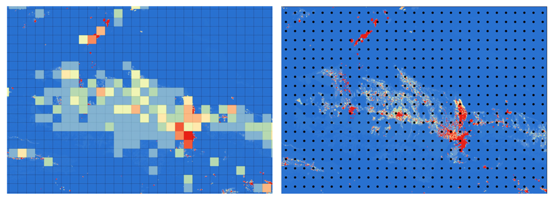
An important assumption in GWR is that there is significant spatial heterogeneity, or non-smoothness, in the spatial relationships of the data. Therefore, when modeling spatial relationships using GWR, the model relationship heterogeneity features need to be tested [26]. Moran’s I was measured using the inverse distance model in spatial autocorrelation analysis (Table 5) [52]. Moran’s I > 0 indicates positive spatial correlation, and the larger its value, the more obvious spatial correlation; Moran’s I < 0 indicates negative spatial correlation, and the smaller its value, the larger the spatial difference; Moran’s I = 0, and the space is random and does not have spatial correlation. The results revealed that Moran’s I > 0 and p = 0, indicating that the distribution of the leisure agriculture exhibited significant spatial correlation. The ordinary least squares (OLS) method was then used to conduct a global regression analysis. The Fishnet tool in ArcGIS 10.4 divided the entire territory into 25 km × 25 km grids, and the image-element values of the raster data were extracted for each grid (Figure 5), resulting in 4848 sets of grid values.
The seven above-mentioned factors were used as the independent variables and leisure agriculture was used as the dependent variable to construct an OLS model for measuring the influences of the factors on each independent leisure agriculture data point variable. Then, the factors with higher significance levels were screened out (Figure 6). The results showed that the variance inflation factor (VIF) values of each independent variable were less than 7.5, and, therefore, there was no collinearity problem between the variables. The goodness of fit was R = 0.44, and the results were significant at the 1% level, according to the F-test, indicating that the constructed model was robust. Five independent variables, i.e., population, rainfall, transportation, tourism resources, and towns, passed the significance test and had positive or negative effects on the distribution of the leisure agriculture to different degrees.
According to the positive and negative attributes of the regression coefficients (Table 6), only the population had a negative relationship with the distribution of the leisure agriculture, while urban, tourism resource, transportation, and rainfall all exhibited significant positive relationships. In terms of the absolute values of the regression coefficients, transportation > urban > tourism resources > population > rainfall. Traffic had the most influence on the distribution of the leisure agriculture, followed by cities, and rainfall had the least influence, as rural areas with convenient transportation can use artificial watering or urban tap water for farmland; however, this also increases the operational costs of leisure agriculture. Therefore, natural rainfall still affected the distribution of the leisure agriculture to a certain extent, but at the lowest level.
The p values of the robust probability statistics for the topographic and economic factors were not significant enough to determine the relationships between them and the number of leisure agriculture points. This could be related to the way leisure agriculture operates; as it tends to be distributed in oases, changes in elevation can hardly have a significant effect on its distribution. In addition, Xinjiang is the largest province in China in terms of area, and the economic zone is concentrated in the urban cluster on the northern slope of the Tianshan Mountains, which does not have an obvious coupling relationship with the distribution of the data points.
After OLS global regression analysis, GWR was further used to explore the local characteristics and spatial heterogeneity of the different factors affecting the distribution of the leisure agriculture. The GWR was conducted using the GWmodelS software to obtain the local parameters for the five factors that passed the OLS test (Table 7). R2 and adjusted R2, after GWR, were 0.841424 and 0.370414, respectively. This is a significant improvement in comparison to the fitted values measured using the OLS method. In addition, the corrected Akaike information criterion (AICc) (Table 8) value decreased from 42,107.87 to 36,210.46, a reduction of 5897.41, which is much greater than 3. Therefore, GWR is more suitable for this study than OLS.
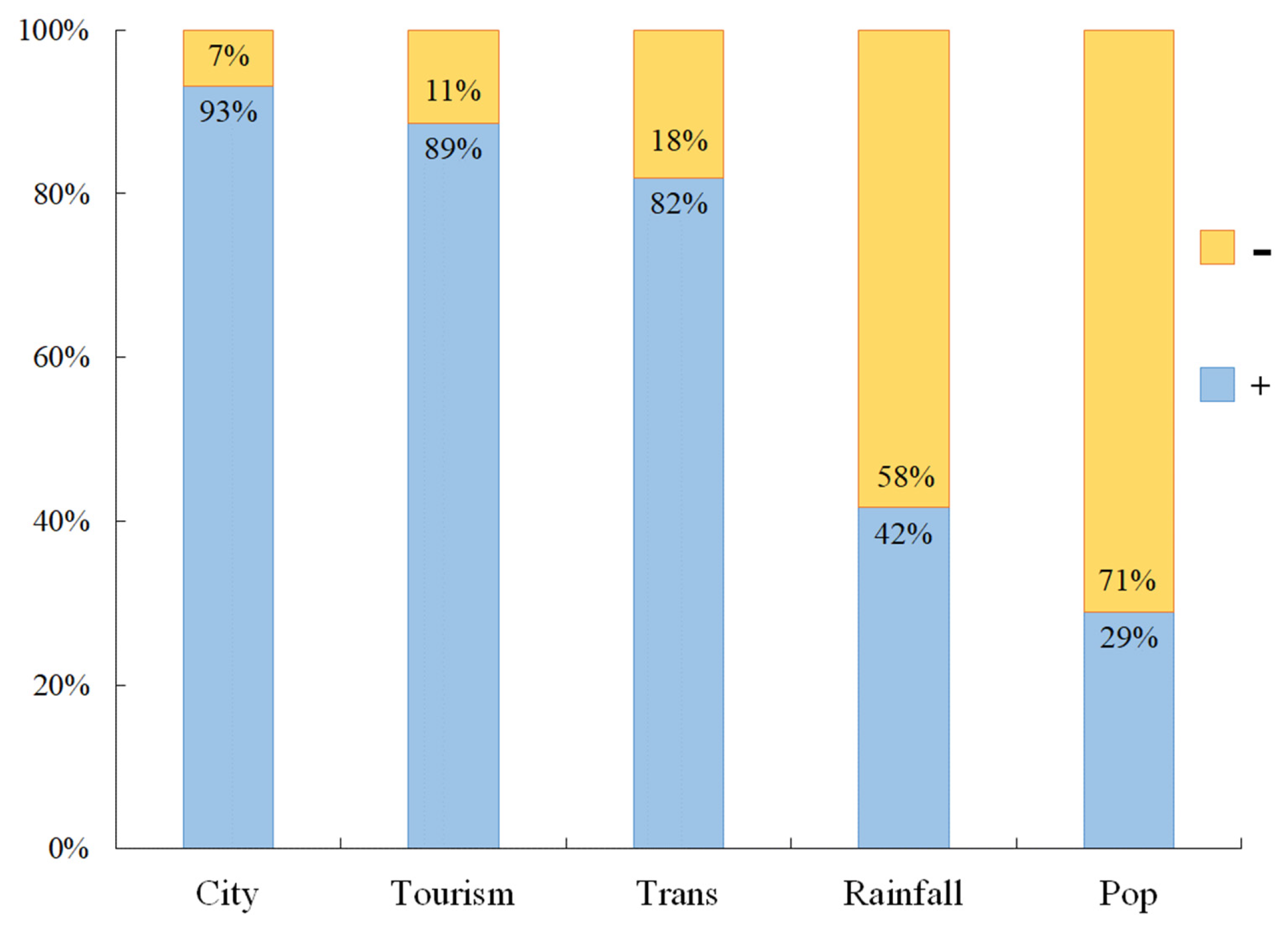
The GWR model counted the regression coefficients among the different spaces in the 4848 grids. Based on the distribution of the positive and negative values of the regression coefficients of each factor, it was found that the spatial variability of the influences of the rainfall and population factors on the distribution of the leisure agriculture was large. These negative relationships reached more than 30%, and the influence on the distribution of the leisure agriculture was complex. The spatial differences in the regression coefficients for factors such as cities, tourism resources, and transportation were small, with more than 80% having positive relationships. These three factors had consistent effects on the spatial distribution of leisure agriculture. The distribution of the regression coefficients was expressed visually, using ArcGIS 10.4, and there was large spatial variability in the effect of each factor on the leisure agriculture.

3.4. Analysis of Effects

3.4.1. Rainfall Factor

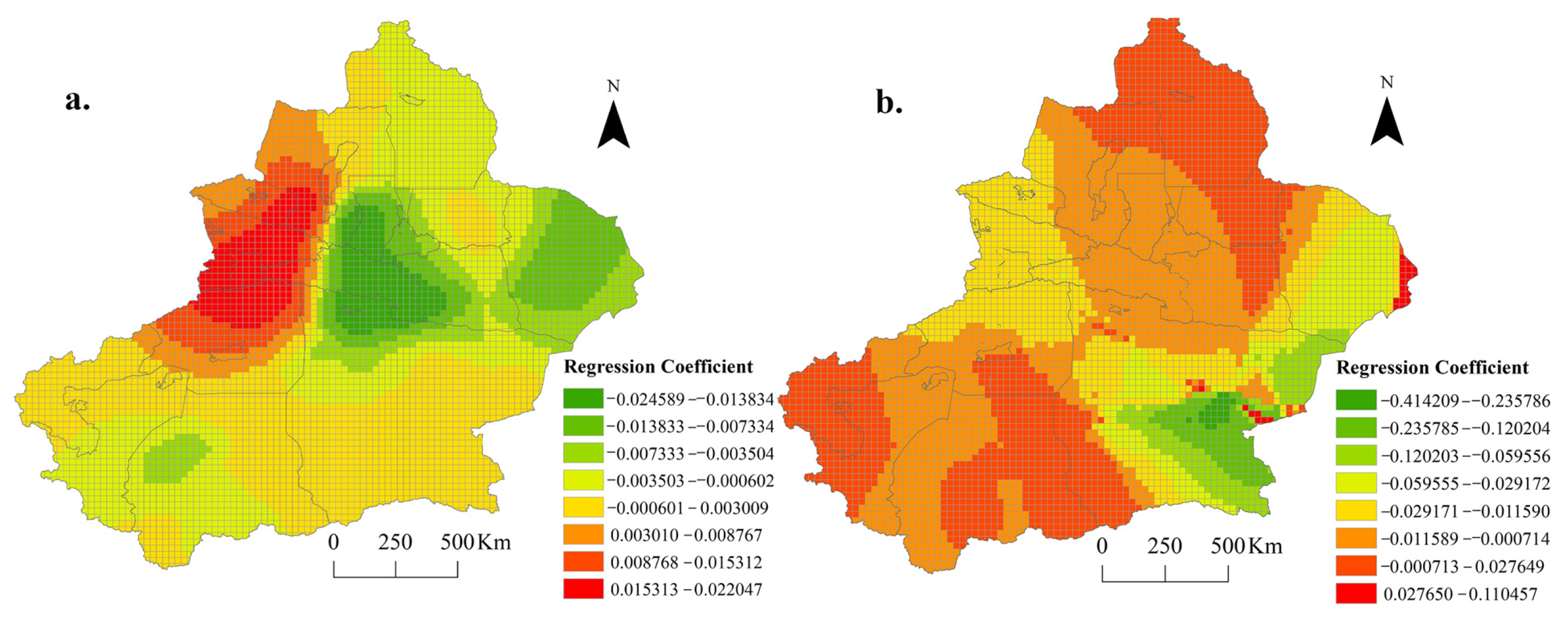
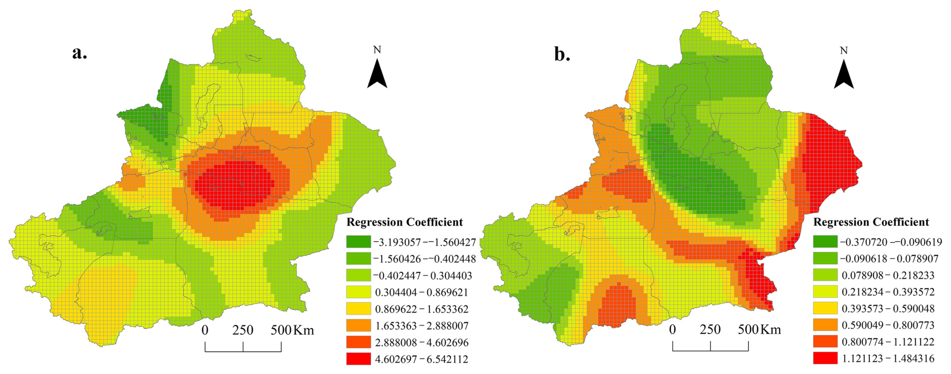
Agricultural development often relies on superior natural conditions and abundant resource endowment, which are demanding on natural elements. Based on the positive and negative values of the regression coefficients of the rainfall elements, the positive attributes accounted for approximately 42% and the negative attributes accounted for 58% (Figure 7). The positive values were mainly distributed in the Ili valley, in western Xinjiang, and extended to the north and south, including Ili, Bortala Mongol Autonomous Prefecture (hereinafter referred to as, Bortala), and Aksu (Figure 8a). These areas are rich in river systems and surround the Tianshan Mountains. Atlantic water vapor enters the Ili Valley and is blocked by the Tianshan Mountains.
Thus, the average annual rainfall can reach 417.6 mm, making it the wettest region in Xinjiang. As a result, it had the largest distribution of leisure agriculture in Xinjiang. It is also one of the three major lavender-growing bases in the world, presenting opportunities for local residents to develop leisure agriculture. The negative areas were concentrated in Urumqi, Turpan, and Hami, in the eastern and central areas of the Tianshan Mountains. All of these areas had little rain (less than 200 mm of annual rainfall), long daylight hours, and few clouds. Turpan, in particular, received less than 40 mm of rainfall and had a cumulative temperature of more than 4000 °C. Leisure agriculture, with locally appropriate characteristics, has developed, subsequently becoming a hotspot for leisure agriculture tourism with geographical characteristics.

3.4.2. Population Factors

The regression coefficient of the influence of the population factors on the leisure agriculture was only 29% in the positive region (Figure 7), i.e., located in the northern, southern, and south-western parts of Xinjiang, forming a high-value area in the easternmost part of Hami (Figure 8b). The rest of Xinjiang exhibited negative values, forming a concentration of negative values in the south-eastern region of Bazhou. This can be attributed to the sparse population in these areas and the fact that the Altai region is bounded by the Altai Mountains, to the north, and the Gurbantunggut Desert to the south. It was not a tourist hotspot. However, under the Altai Mountains, there is abundant flowing water, and leisure agriculture that relies on water conditions has gradually emerged. In addition, the south-eastern part of Bazhou had a fragile environment, a small population, and scattered leisure agriculture spots. This area is located in Ruoqiang County, which had a population of only 80,000 at the end of 2020, with an altitude of 768–6900 m, undulating terrain, and mountainous areas in the south. The plantation agriculture area was distributed in the alluvial fan oasis area, in the central part of Ruoqiang, and the agricultural carrying capacity was not sufficient to support its transformation into a leisure agriculture model. However, this area had numerous monuments and natural scenic resources, such as rare alpine areas and Yin Yang Lake, and low-level farmhouses have emerged to meet the basic needs of tourists by relying on the natural landscape.

3.4.3. Traffic Factors

Traffic is important for connecting leisure agriculture tourism with the source market. The positive correlation effect of the transportation factor on the distribution of leisure agriculture was approximately 82%, while the negative value was only 18% (Figure 7). The distribution of the regression coefficients across all of Xinjiang (Figure 9a) revealed a clear high-value area in and around Korla. A decreasing trend was observed moving outward from this center, and a ring-shaped negative area formed around the high-value area. This indicates that the influence of traffic factors on leisure agriculture changed from positive to negative, with Korla as the center. Korla is located in the northern part of Bazhou. This region had good accessibility, thus promoting leisure agriculture development. The pear of Korla is an important local agricultural product, and is supplied to the entire country and globally. Therefore, leisure agriculture in this area tended to be positively influenced by the traffic factor. In addition, about 18% of the negative areas were distributed in the western border areas of Xinjiang, such as Kashgar, Kezhou, Ili, and Bortala. All of these areas were negatively affected by the traffic factor. This could be related to transportation peculiarities, as border transportation is often used for resource deployment and defense needs, thus weakening the agglomeration effect on leisure agriculture. In contrast, the leisure agriculture was distributed in rural areas far from large-scale transportation facilities. These areas contained famous natural scenic spots, which were used to develop leisure agriculture and attract tourists.

3.4.4. Tourism-Resource Factors

The positive effect of tourism resources on the distribution of leisure agriculture was second only to that of the urban element. The distribution of the positive regression coefficients occupied approximately 89% of the study area, while the negative coefficients only accounted for 11% (Figure 7). A clear strip-like high-value area occurred in eastern and central Xinjiang, while a semicircular high-value area was formed in the Hotan area in the south (Figure 9b). The landform type of the substrate distributed in the high-value area was mainly desert, or was located near high mountains, with few towns, making the conditions unsuitable for agriculture. These places also lacked tourism resources. Therefore, these places were not suitable for leisure agriculture that depends on tourism resources, thus forming a blank area of leisure agriculture. In addition, substantial tourism resources were distributed in places such as Ili and northern Aksu, which are primarily made up of natural scenery, such as lakes, grasslands, and deserts. The rural residents in these places could develop leisure agriculture based on tourism resources to attract tourists to spend money. The negative area was mainly concentrated in the block area centered on Korla in central Xinjiang, which straddles the Tianshan Mountains and contains natural tourism resources, such as canyons and glaciers. However, there is an alpine basin where the eastern and western branches of the Tianshan Mountains intersect, which is not suitable for leisure agriculture. In addition, there were large negative areas in northern Xinjiang, such as Karamay, Urumqi, and Tacheng. They mostly fluctuated around 0, indicating that tourism resources had a weak effect. Tourism resources and leisure agriculture could operate separately around cities such as Urumqi.

3.4.5. City Distribution Factors

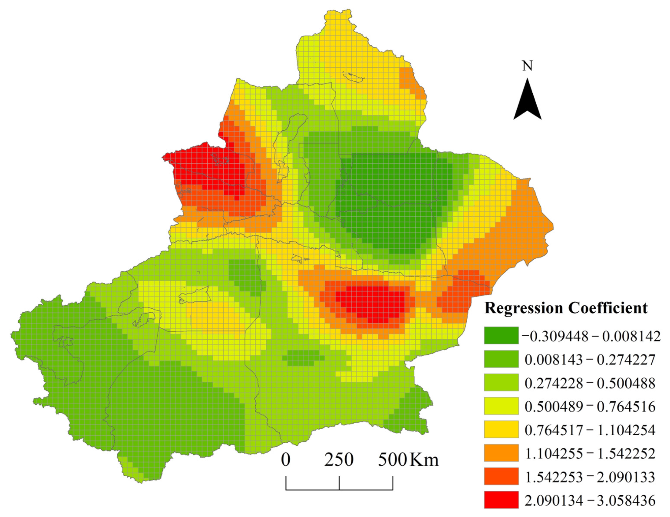
The city distribution factors and the distribution of leisure agriculture points exhibited a positive correlation in approximately 93% of the region, while the negative correlation areas only accounted for 17% (Figure 7). This indicates that the distribution of leisure agriculture revolved around areas closer to the cities. The spatial distribution showed that the high regression coefficients of the city distribution factors were mainly concentrated in central Xinjiang, which is an important economic belt, and is an economic corridor connecting China with the countries to the west. The service groups for leisure agriculture were mainly the domestic urban population and foreign tourists. The wide distribution of towns and cities contributed to the high concentration of market-oriented leisure agriculture in this area. The healthy development of leisure agriculture requires the infrastructure provided by cities. The only negative area was located in the Tuha Basin (Figure 10). There are two possible reasons for this phenomenon. First, the Tuha Basin is one of the three major oil-bearing basins in Xinjiang [53]; therefore, the industry in this area is primarily based on the energy industry, making it a core area for supplying energy to the surrounding cities. Second, the landscape is mostly desert, and secondary industries dependent on agriculture are not easily formed.

4. Discussion

In China, particularly in rural areas, leisure agriculture has become an important part of tourism development [54]. The alternative sightseeing sites provided by leisure agriculture cannot be duplicated in urban tourism. Previously, the relationship between leisure agriculture and rural tourism has only been granted a weak association, which has not yet achieved the integration and upgrading of industries and fails to achieve the ultimate purpose of driving rural economic development [55].
In this study, it was found that the leisure agriculture in Xinjiang exhibited agglomeration characteristics and uneven spatial distribution. This unevenness was related to natural factors, such as rainfall and geomorphology. The traditional view is that natural factors are the intrinsic determinants that influence the distribution of features, while social factors are the extrinsic drivers [56]. However, in this study, it was found that the largest absolute values of the regression coefficients were for transportation, followed by cities, tourism resources, and population. The topographic factors were not found to be significantly correlated in the OLS model. With technological advances, social factors now have more influence on leisure agriculture than natural factors [57]. Social factors not only attract the spatial distribution of the leisure agriculture, but also promote sustainable social development. Therefore, leisure agriculture has transitioned from a resource-driven model to capital-driven and market-driven models. Socio-economic factors such as city distribution, population, transportation, and tourism resources were found to be closely related to the development of the leisure agriculture in Xinjiang [58]. In addition, greater use can be made of the attractiveness of tourism resources to population sources; this type of leisure agriculture is mostly market-driven. Leisure agriculture should take on different forms based on the different driving modes, in terms of the target population and development mode, suitable for a particular area. Thus, places such as Ili and Bortala should seize policy opportunities to broaden their agricultural industry chains and transform resource advantages into economic advantages [59].
The development of leisure agriculture still faces a number of problems. The sustainability of leisure agriculture and rural tourism in Xinjiang is still, overall, at a poor stage, which needs a lot of work to drive the sustainable development path of leisure agriculture into a robust stage [60].
Meanwhile, since 2018, China has issued 103 documents with “leisure agriculture” as a keyword at the national level and 84 documents at the Xinjiang level. Various measures have been proposed for rural travel development, including enhancing the construction role of village enterprises, using community management, and increasing information technology services, with government management remaining the dominant force [61]. Government policies for attracting investment and promoting the layout of projects have accelerated the integration of tourism and agriculture, focusing on solving the mismatch between land factor inputs and economic output [62].
In addition, differences in the types of leisure agriculture can lead to different factors affecting the spatial distribution [33]. Depending on the degree of influence and the targeted customer groups, these can be broadly classified as traffic proximity, suburban, population-oriented, and tourism-driven types. The scale, grade, and customer characteristics of the different types of leisure agriculture vary. The traffic-proximity type often relies on airports, high-speed railways, and highways, and its primary business comes from providing tourists who are on the road with a break and to sell them agricultural products. The suburban type is distributed in the suburbs of cities [35] and is oriented toward the opening of pick-your-own-vegetable businesses and farmland parks for tourists. Its scale is larger than those of the other types. The population-oriented type belongs to the transitional peri-urban and tourism-resource types. Leisure agriculture tourism facilities are specifically built by villagers to broaden their income channels. These are distributed in rural areas around cities or tourist attractions, and they can reduce business costs and may be positioned close to the source market. The tourism-driven type of leisure agriculture is developed within a scenic area, or in the rural areas surrounding a scenic area, providing a wider range of businesses for visitors, such as dining, lodging, transportation, and entertainment.

5. Conclusions

Based on the analysis of 1745 leisure agriculture points in Xinjiang, the factors affecting their spatial distribution were explored using GWR. The main conclusions of this study are summarized below.
(1)
The spatial distribution of the leisure agriculture spots in Xinjiang was uneven. The distribution was concentrated to the north and south of the Tianshan Mountains, in western Xinjiang. The number of sites varied significantly between different locations, with more than half of the sites concentrated in Ili and north-western Bazhou and fewer in Kezhou, Karamay, and Turpan.
(2)
In terms of the spatial distribution density, four high-concentration centers and one secondary concentration center were identified. The four high-concentration centers were located near Bosten Lake, in Hami, and on the east and west sides of the Ili River Valley. The secondary concentration center was located in Urumqi and radiated outward toward the surrounding areas. Overall, the leisure agriculture in Xinjiang was found to be distributed, predominantly, on either side of the Tianshan Mountains and in the Ili River Valley in the west. The overall number of sites decreased to the south.
(3)
Seven factors were selected and used to quantify the variability of their effects using OLS and GWR. The results revealed that the population, transportation, tourism resources, city distribution factors, and rainfall factors had significant effects on the distribution of the leisure agriculture. According to the positive and negative values of the regression coefficients, all of the factors had negative and positive effects on the distribution of the leisure agriculture and formed high- and low-value areas. This indicates that there was significant local variability in the degree and direction of the influences of the factors on the distribution of the leisure agriculture. The effects of the topography and economy on the distribution of leisure agriculture were not obvious.
(4)
The leisure agriculture had different degrees of response to the different factors, exhibiting considerable internal variability. Compared with the other factors, the spatial variability of the effects of rainfall on the spatial distribution of the leisure agriculture were greater, with a considerable proportion of both positive and negative effects. The traffic, urban, and tourism-resource factors all had consistent effects on the distribution of the leisure agriculture. The directional effects were largely positive, with positive regression coefficients in more than 80% of the study area. The population factors, on the other hand, are dominated by negative effects. In terms of the range of the geographical effects, the positive high-value areas of the rainfall factor were distributed in western Xinjiang in the Ili Valley, Kezhou, and Bortala. The negative values were primarily distributed in eastern Xinjiang in Urumqi, Turpan, and Hami. The negative areas for the population factors accounted for a large proportion. The high regression coefficient values of the traffic factor were centered on the north-western part of Bazhou and the values decreased, outward, in a belt-like manner. For the urban factor, Bosten Lake and the Ili Valley in Bazhou were the positive high-value concentration areas. The positive values were also distributed in Altai, in the north and Hami in the east, with a negative value center forming a ring around Urumqi, Changji, and Turpan. The positive high-value areas of the tourism-resource factors were distributed along the border in eastern Xinjiang. In addition, a belt-like high-value area was formed from the south-eastern part of Bazhou, toward the Ili Valley.
To summarize, the distribution of leisure agriculture has explicit correlation with several factors. To develop tourism through leisure agriculture, it is necessary to solve the contradiction between agriculture, rural areas and farmers, in order to promote the transformation of traditional agriculture into leisure agriculture and modern urban agriculture. Secondly, the construction of road networks should be improved in order to promote the mutual integration of tourism resources. Transportation is the necessary foundation for the development of leisure agriculture, and the distribution along transportation routes is one of the main features of the leisure agriculture distribution in Xinjiang; finally, we should rely on central cities to promote the reasonable layout of population and economy.

Author Contributions

All of the authors (Y.C., D.L., Z.S., S.Y. and Y.R.) contributed to the design of the research, the writing and revision of the manuscript, and the analysis of the data. All authors have read and agreed to the published version of the manuscript.

Funding

This research was funded by the National Natural Science Foundation of China (Grant No. 41661036), the National Natural Science Foundation of China—Xinjiang Joint Fund (Grant No. U1603241), and the overseas study support project of the Xinjiang local government (No. 117/40299006).

Institutional Review Board Statement

Not applicable.

Informed Consent Statement

Not applicable.

Data Availability Statement

Data is contained within the article.

Acknowledgments

Thank you to the hard-working editors and reviewers for their valuable comments.

Conflicts of Interest

The authors declare no conflict of interest.

References

  1. Pillay, M.; Rogerson, C.M. Agriculture-tourism linkages and pro-poor impacts: The accommodation sector of urban coastal KwaZulu-Natal, South Africa. Appl. Geogr. 2013, 36, 49–58. [Google Scholar] [CrossRef]
  2. Ma, X.; Han, M.; Luo, J.; Song, Y.; Chen, R.; Sun, X. The empirical decomposition and peak path of China’s tourism carbon emissions. Environ. Sci. Pollut. Res. 2021, 28, 66448–66463. [Google Scholar] [CrossRef] [PubMed]
  3. Dodman, D.; Rhiney, K. “We nyammin?” food supply, authenticity, and the tourist experience in Negril, Jamaica. In New Perspectives in Caribbean Tourism; Routledge: New York, NY, USA, 2008; pp. 115–133. [Google Scholar] [CrossRef]
  4. Ćirić, M.; Tešanović, D.; Kalenjuk Pivarski, B.; Ćirić, I.; Banjac, M.; Radivojević, G.; Grubor, B.; Tošić, P.; Simović, O.; Šmugović, S. Analyses of the Attitudes of Agricultural Holdings on the Development of Agritourism and the Impacts on the Economy, Society and Environment of Serbia. Sustainability 2021, 13, 13729. [Google Scholar] [CrossRef]
  5. Vasadze, M. The Role of Agritourism in Sustainable Rural Development of Georgia. China-USA Bus. Rev. 2020, 19, 141–147. [Google Scholar] [CrossRef]
  6. Klak, T. Tourism and agriculture: New geographies of consumption, production and rural restructuring. J. Lat. Am. Geogr. 2012, 11, 183–184. [Google Scholar] [CrossRef] [Green Version]
  7. Asiedu, A.B.; Gbedema, T.K. The nexus between agriculture and tourism in Ghana: A case of underexploited development potential. In Tourism and Agriculture: New Geographies of Production and Rural Restructuring; Routledge: London, UK, 2011; pp. 28–46. [Google Scholar]
  8. An, W.; Alarcón, S. How Can Rural Tourism Be Sustainable? A Systematic Review. Sustainability 2020, 12, 7758. [Google Scholar] [CrossRef]
  9. Guo, Y.; Jiang, J.; Li, S. A Sustainable Tourism Policy Research Review. Sustainability 2019, 11, 3187. [Google Scholar] [CrossRef] [Green Version]
  10. Tang, C.; Wan, Z.; Ng, P.; Dai, X.; Sheng, Q.; Chen, D. Temporal and spatial evolution of carbon emissions and their influencing factors for tourist attractions at Heritage tourist destinations. Sustainability 2019, 11, 5944. [Google Scholar] [CrossRef] [Green Version]
  11. Amsden, B.; McEntee, J. Agrileisure: Re-imagining the relationship between agriculture, leisure, and social change. Leis. Loisir 2011, 35, 37–48. [Google Scholar] [CrossRef]
  12. Long, H.; Zhang, Y.; Tu, S. Rural vitalization in China: A perspective of land consolidation. J. Geogr. Sci. 2019, 29, 517–530. [Google Scholar] [CrossRef] [Green Version]
  13. Liu, Y.; Guo, Y.; Zhou, Y. Poverty alleviation in rural China: Policy changes, future challenges and policy implications. China Agric. Econ. Rev. 2018, 10, 241–259. [Google Scholar] [CrossRef] [Green Version]
  14. Yang, J.; Yang, R.; Chen, M.-H.; Su, C.-H.J.; Zhi, Y.; Xi, J. Effects of rural revitalization on rural tourism. J. Hosp. Tour. Manag. 2021, 47, 35–45. [Google Scholar] [CrossRef]
  15. Li, J.; Liu, Y.; Yang, Y.; Jiang, N. County-rural revitalization spatial differences and model optimization in Miyun District of Beijing-Tianjin-Hebei region. J. Rural Stud. 2021, 86, 724–734. [Google Scholar] [CrossRef]
  16. Chen, Y.; Wen, C.; Xu, X. The COVID-19 Impact on Population Flow of Ethnic Minority Areas. J. Univ. Electron. Sci. Technol. China 2021, 50, 938–946. [Google Scholar] [CrossRef]
  17. Boccia, F.; Sarnacchiaro, P. Chi-squared automatic interaction detector analysis on a choice experiment: An evaluation of responsible initiatives on consumers’ purchasing behavior. Corp. Soc. Responsib. Environ. Manag. 2019, 27, 1143–1151. [Google Scholar] [CrossRef]
  18. Wu, H.C.; Lin, Y.C.; Chen, T.C.T. Leisure Agricultural Park Selection for Traveler Groups Amid the COVID-19 Pandemic. Agriculture 2022, 12, 111. [Google Scholar] [CrossRef]
  19. Roman, M.; Grudzień, P. The Essence of Agritourism and Its Profitability during the Coronavirus (COVID-19) Pandemic. Agriculture 2021, 11, 458. [Google Scholar] [CrossRef]
  20. Nie, J.; Kiminami, A.; Yagi, H. Exploring the Sustainability of Urban Leisure Agriculture in Shanghai. Sustainability 2022, 14, 4813. [Google Scholar] [CrossRef]
  21. Martínez, J.M.G.; Martín, J.M.M.; Fernández, J.A.S.; Mogorrón-Guerrero, H. An analysis of the stability of rural tourism as a desired condition for sustainable tourism. J. Bus. Res. 2019, 100, 165–174. [Google Scholar] [CrossRef]
  22. Cui, J.; Li, R.; Zhang, L.; Jing, Y. Spatially illustrating leisure agriculture: Empirical evidence from picking orchards in China. Land 2021, 10, 631. [Google Scholar] [CrossRef]
  23. Bhatta, K.; Itagaki, K.; Ohe, Y. Determinant factors of farmers’ willingness to start agritourism in rural Nepal. Open Agric. 2019, 4, 431–445. [Google Scholar] [CrossRef]
  24. Stokowski, P.A.; Kuentzel, W.F.; Derrien, M.M.; Jakobcic, Y.L. Social, cultural and spatial imaginaries in rural tourism transitions. J. Rural Stud. 2021, 87, 243–253. [Google Scholar] [CrossRef]
  25. Kim, S.; Lee, S.K.; Lee, D.; Jeong, J.; Moon, J. The effect of agritourism experience on consumers’ future food purchase patterns. Tour. Manag. 2019, 70, 144–152. [Google Scholar] [CrossRef]
  26. Lu, B.; Ge, Y.; Qin, K.; Zheng, J. A Review on Geographically Weighted Regression. Geomat. Inf. Sci. Wuhan Univ. 2020, 45, 1356–1366. [Google Scholar] [CrossRef]
  27. Zhou, Q.; Wang, C.; Fang, S. Application of geographically weighted regression (GWR) in the analysis of the cause of haze pollution in China. Atmos. Pollut. Res. 2019, 10, 835–846. [Google Scholar] [CrossRef]
  28. Gu, P. Analysis of the impacts of COVID-19 pandemic on leisure agriculture and rural tourism in Zhengzhou and the countermeasures. Front. Soc. Sci. Technol. 2020, 2, 89–96. [Google Scholar]
  29. Liu, F.; Wang, J.; Liu, J.; Li, Y.; Liu, D.; Tong, J.; Li, Z.; Yu, D.; Fan, Y.; Bi, X. Predicting and analyzing the COVID-19 epidemic in China: Based on SEIRD, LSTM and GWR models. PLoS ONE 2020, 15, e0238280. [Google Scholar] [CrossRef]
  30. Sulekan, A.; Suhaila, J.; Wahid, N.A.A. Geographically Weighted Regression on dengue epidemic in Peninsular Malaysia. J. Phys. Conf. Ser. 2021, 1988, 012099. [Google Scholar] [CrossRef]
  31. Brunsdon, C.; Fotheringham, S.; Charlton, M. Geographically weighted regression. J. R. Stat. Soc. Ser. D Stat. 1998, 47, 431–443. [Google Scholar] [CrossRef]
  32. Xu, C.; Zhao, J.; Liu, P. A geographically weighted regression approach to investigate the effects of traffic conditions and road characteristics on air pollutant emissions. J. Clean. Prod. 2019, 239, 118084. [Google Scholar] [CrossRef]
  33. Wang, J.; Guo, J.; Liu, Y.; Lu, G.; Feng, L. Spatial distribution characteristics and influencing factors of ski resorts in China. Geogr. Res. 2022, 41, 390–405. [Google Scholar] [CrossRef]
  34. Casolani, N.; Cartone, A.; Postiglione, P.; Liberatore, L. Climate variability in agriculture and crop water requirement: Spatial analysis of Italian provinces. J. Clean. Prod. 2020, 262, 121331. [Google Scholar] [CrossRef]
  35. Zhong, A.; Hu, B.; Wang, C.; Xue, D.; He, E. The Impact of Urbanization on urban agriculture: Evidence from China. J. Clean. Prod. 2020, 276, 122686. [Google Scholar] [CrossRef]
  36. Qiao, H.; Wang, C.; Chen, M.H.; Su, C.H.J.; Tsai, C.H.K.; Liu, J. Hedonic price analysis for high-end rural homestay room rates. J. Hosp. Tour. Manag. 2021, 49, 1–11. [Google Scholar] [CrossRef]
  37. Chai, Z.; Yibo, Y.; Simayi, Z.; Yang, S.; Abulimiti, M.; Yuqing, W. Carbon emissions index decomposition and carbon emissions prediction in Xinjiang from the perspective of population-related factors, based on the combination of STIRPAT model and neural network. Environ. Sci. Pollut. Res. 2022, 29, 31781–31796. [Google Scholar] [CrossRef]
  38. ThiNguyen, H.A.; Gheewala, S.H.; Sophea, T.; Areerob, T. Comparative carbon footprint assessment of agricultural and tourist locations in Thailand. J. Clean. Prod. 2020, 269, 122407. [Google Scholar] [CrossRef]
  39. Belliggiano, A.; Garcia, E.C.; Labianca, M.; Valverde, F.N.; De Rubertis, S. The “eco-effectiveness” of agritourism dynamics in Italy and Spain: A tool for evaluating regional sustainability. Sustainability 2020, 12, 7080. [Google Scholar] [CrossRef]
  40. Goh, H.C. Strategies for post-COVID-19 prospects of Sabah’s tourist market–Reactions to shocks caused by pandemic or reflection for sustainable tourism? Res. Glob. 2021, 3, 100056. [Google Scholar] [CrossRef]
  41. Chang, Y.; Li, D.; Simayi, Z.; Yang, S.; Abulimiti, M.; Ren, Y. Spatial Pattern Analysis of Xinjiang Tourism Resources Based on Electronic Map Points of Interest. Int. J. Environ. Res. Public Health 2022, 19, 7666. [Google Scholar] [CrossRef]
  42. Bahtebay, J.; Zhang, F.; Ariken, M.; Chan, N.W.; Tan, M.L. Evaluation of the coordinated development of urbanization-resources-environment from the incremental perspective of Xinjiang, China. J. Clean. Prod. 2021, 325, 129309. [Google Scholar] [CrossRef]
  43. Li, D.; Cao, F.; Yang, C. Spatial Distribution Charactertistics of Leisure Agriculture in Liaoning Province. North. Hortic. 2020, 165–171. [Google Scholar] [CrossRef]
  44. Peng, J.; Cao, Y. Coordination of spatial relationship between population and economy in yili prefecture in Xinjing. J. Southwest Univ. Nat. Sci. Ed. 2022, 44, 183–193. [Google Scholar] [CrossRef]
  45. Guo, Y.; Min, L. Classification and spatial distribution characteristics of tourist attractions in Shanxi Province based on POI data. Sci. Geogr. Sin. 2021, 41, 1246–1255. [Google Scholar] [CrossRef]
  46. Yang, J.; Zhu, J.; Sun, Y.; Zhao, J. Delimitating Urban Commercial Central Districts by Combining Kernel Density Estimation and Road Intersections: A Case Study in Nanjing City, China. Int. J. Geo-Inf. 2019, 8, 93. [Google Scholar] [CrossRef] [Green Version]
  47. Wang, B.; Shi, W.; Miao, Z. Confidence analysis of standard deviational ellipse and its extension into higher dimensional Euclidean space. PLoS ONE 2015, 10, e0118537. [Google Scholar] [CrossRef]
  48. Huang, Q.; Bo, Y.; Xiongbo, G.; Lili, L.; Bin, W.; Ying, C.; Huifang, Y.; Xiaoyan, Z. Analysis on Spatial Pattern of Tourist Attractions in Changsha City Based on POI Data. J. Nat. Sci. Hunan Norm. Univ. 2021, 44, 40–49. [Google Scholar]
  49. Liu, Y.; He, Z.; Zhou, X. Space-Time Variation and Spatial Differentiation of COVID-19 Confirmed Cases in Hubei Province Based on Extended GWR. Int. J. Geo-Inf. 2020, 9, 536. [Google Scholar] [CrossRef]
  50. Wei, T. Research on income inequality in China—An analysis by Lorenz curve. Stud. Sci. Sci. 2007, 96–99. [Google Scholar]
  51. Dongran, S.; Lei, X. A study on the current situation and equity of nursing human resources allocation in Zhejiang Province. Mod. Hosp. Manag. 2018, 16, 54–56. [Google Scholar] [CrossRef]
  52. Zhang, L.; Leng, L.; Zeng, Y.; Lin, X.; Chen, S. Spatial distribution of rural population using mixed geographically weighted regression: Evidence from Jiangxi Province in China. PLoS ONE 2021, 16, e0250399. [Google Scholar] [CrossRef]
  53. Jia, C.; Zou, C.; Yang, Z.; Zhu, R.; Chen, Z.; Zhang, B.; Jiang, L. Significant progress of continental petroleum geological theory in basins of Central and Western China. Pet. Explor. Dev. 2018, 45, 573–588. [Google Scholar] [CrossRef]
  54. Yang, J. The Influence and Measures of Developing Sightseeing and Leisure Agriculture on Rural Economic Development. IOP Conf. Ser. Earth Environ. Sci. 2020, 526, 012061. [Google Scholar] [CrossRef]
  55. Ma, Y.; Wang, C. Path of the County-level Agritourism Development in Xinjiang under the Background of Rural Revitalization Strategy. Agric. Outlook 2022, 18, 114–118. [Google Scholar]
  56. Sun, S.; Lui, B.; Guo, Z.; Wang, F.; Wang, X.; Qiu, Z. Evolution of Spatial Distribution Characteristics and Influencing Factors of Skiing Resorts in China Since Reform and Opening Up. J. Shenyang Sport Univ. 2019, 38, 8–15. [Google Scholar] [CrossRef]
  57. Kapera, I. Sustainable tourism development efforts by local governments in Poland. Sustain. Cities Soc. 2018, 40, 581–588. [Google Scholar] [CrossRef]
  58. Chin, W.L.; Pehin Dato Musa, S.F. Agritourism resilience against COVID-19: Impacts and management strategies. Cogent Soc. Sci. 2021, 7, 1950290. [Google Scholar] [CrossRef]
  59. Morales-Zamorano, C.-G.; Bustamante-Valenzuela, A.L.; Suarez-Hernández, A.C.; Morales, L. Intangible Resources in Sustainable Agritourism: As A Competitive Advantage. J. Bus. Econ. 2020, 11, 561–569. [Google Scholar] [CrossRef]
  60. Bai, X.; Peng, Y. Assessment of Sustainable Development of County-Level Agritourism and Countryside Tourism in Xinjiang. Chin. J. Agric. Resour. Reg. Plan. 2020, 41, 304–310. [Google Scholar]
  61. Purnomo, S.; Rahayu, E.S.; Riani, A.L.; Suminah, S.; Udin, U. Empowerment model for sustainable tourism village in an emerging country. J. Asian Financ. Econ. 2020, 7, 261–270. [Google Scholar] [CrossRef]
  62. Zhou, Y.; Xia, J.; Gong, Q.; Wang, Z. Evaluation of Leisure Agriculture Efficiency and Development Path Innovation under the Supply Side Horizon: Survey Data from Huangpi District. In Proceedings of the 2020 3rd International Seminar on Education Research and Social Science (ISERSS 2020), Kuala Lumpur, Malaysia, 24–26 December 2020; pp. 107–114. [Google Scholar]
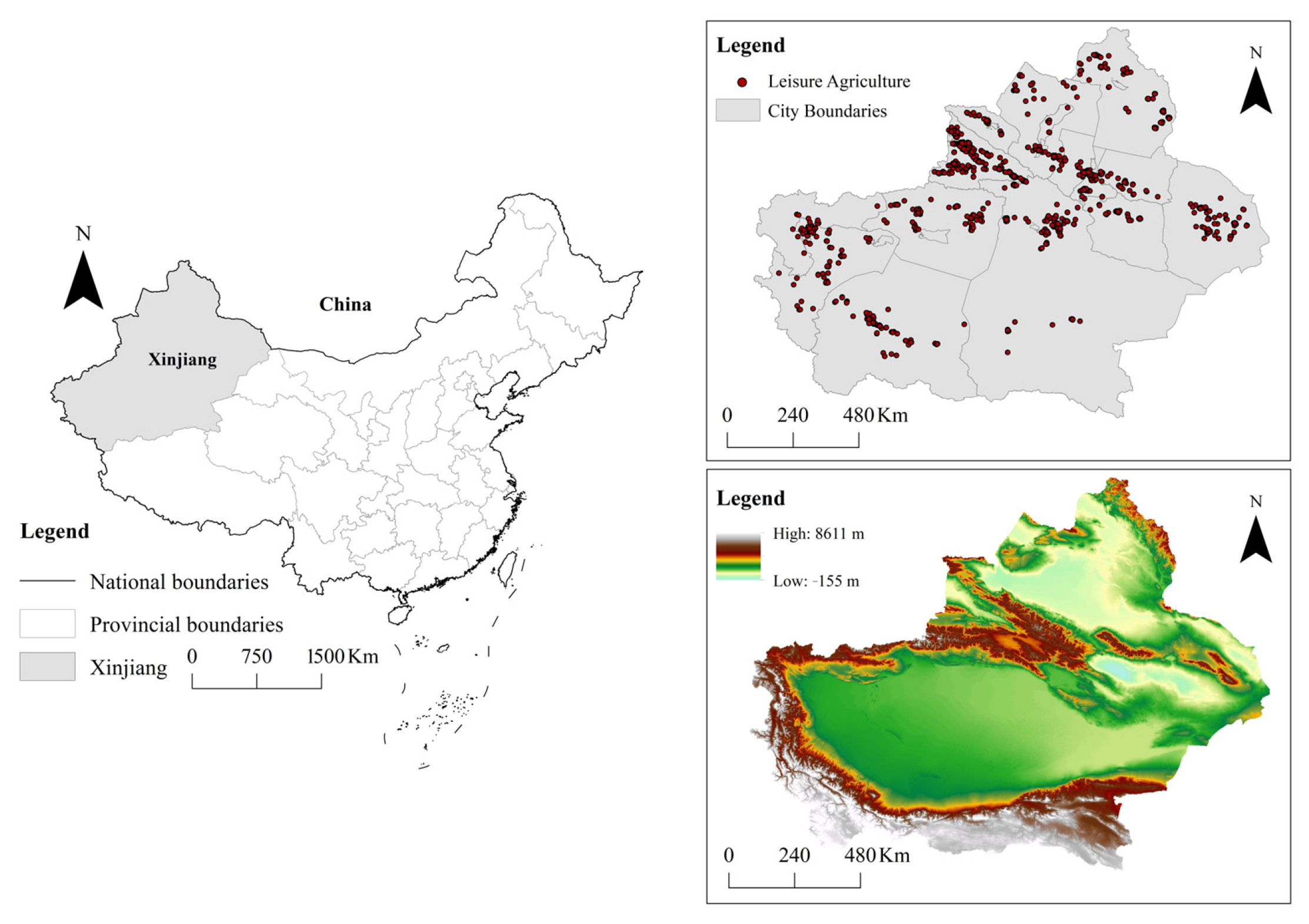
Figure 1. Map of the study area.
Sustainability 14 15002 g001
Figure 2. Spatial distribution of leisure agriculture and standard deviation ellipses.
Sustainability 14 15002 g002
Figure 3. Lorenz curve of the distribution of leisure agriculture in Xinjiang.
Sustainability 14 15002 g003
Figure 4. Kernel density distribution of leisure agriculture.
Sustainability 14 15002 g004
Figure 5. Extraction of image-element values and assignment of values to the grids.
Sustainability 14 15002 g005
Figure 6. Model construction and analysis process.
Sustainability 14 15002 g006
Figure 7. Positive and negative values of regression coefficients for each factor.
Sustainability 14 15002 g007
Figure 8. Distribution of regression coefficients of the (a) rainfall factors and (b) population factors.
Sustainability 14 15002 g008
Figure 9. Distribution of the regression coefficients of (a) transportation factors and (b) tourism-resource factors.
Sustainability 14 15002 g009
Figure 10. Distribution of the regression coefficients of city factors.
Sustainability 14 15002 g010
Table 1. Data sources.
Data CategoriesThe Required DataSource
Natural factorsDEM (30 m)Geospatial Data Cloud (accessed on 13 May 2019)
(https://www.gscloud.cn/)
Rainfall grid dataResource and Environmental Science, Chinese Academy of Sciences Science and Data Center (accessed on 22 June 2022)
(https://www.resdc.cn/)
Socio-economic factorsPopulation grid data
Economic grid data
Traffic line vector dataNational Geomatics Center of China (accessed on 18 June 2022)
(http://www.ngcc.cn/ngcc/)
City point data
Tourist spot dataXinjiang Culture and Tourism Department (accessed on 5 June 2022)
(http://wlt.xinjiang.gov.cn/)
Leisure agriculture points15-March-2022Bigemap GIS Office (accessed on 15 March 2022)
(http://www.bigemap.com/)
Gaode Map (accessed on 15 March 2022)
(https://www.amap.com/)
Base map data8-October-2020National Geomatics Center of China (accessed on 8 October 2020)
(http://www.ngcc.cn/ngcc/)
Table 2. Spatial distribution characteristic index calculation results.
IndexValue
Nearest-neighbor index (R)0.179276
Geographic concentration index (G)37.62259
Imbalance index (S)0.480361
Table 3. Local parameters of the standard deviation ellipse analysis.
ParameterValue
Center-X84.607181
Center-Y42.943143
X-StdDist2.868473
Y-StdDist6.312403
Rotation76.27624
Table 4. Variables and calculation methods for geographically weighted regression.
VariableSymbolIndicatorMaxMinMeanProcessing Method
Dependent
variables
YNumber of
leisure
agriculture points
241.70120.9Number of
leisure
agriculture points in each grid
Independent
variables
GDPEconomic factors17,647.908824.0Grid extraction of image-element values of economic grid data
RainfallRainfall
factors
6616473331.5Grid extraction of image-element values of rainfall grid data
POPPopulation
factors
24,277012,138.5Grid extraction of image-element values of population grid data
DEMTopographic
factors
86111554383Mesh extraction of image-element values of terrain mesh data
TourTourism
resources
692.70346.4Grid extraction of image-element values of the distribution density of tourist points
CityUrban factors178.7089.4Grid extraction of image-element values of town point distribution density
TransTraffic factors50.2025.1Grid extraction of image-element values of traffic line distribution density
Table 5. Parameters of spatial autocorrelation analysis.
ParameterWidth (30 km)
Moran’s I0.25754
Z-score4.832902
p value0.000000
Except value−0.011364
Variance0.003096
Table 6. OLS modeling results.
VariableCoefficientStandard Deviationp Valuet-ValueVIF
Constant−3.616290.5503670.000 ***−6.57069-
Pop−0.005910.002180.070 **−2.710672.315714
DEM−0.000370.0001970.160−1.878221.123668
GDP−0.001380.0012660.275−1.091052.448987
Rainfall0.0043320.0002750.000 ***15.73141.116986
Trans1.6019670.1112430.000 ***14.400564.46111
Tours0.0453940.0104660.000 ***4.3374152.743930
City0.4455480.042070.000 ***10.590724.797246
R20.443132
Adjusted R2
Koenker (BP)
0.442327
860.82529 *
Note: When the Koender (BP) statistic is significant, i.e., when labelled *.The statistical significance of the independent variable needs to be judged based on the robust p value, ** and *** indicate that the variable is statistically significant at the, 5% and 1% levels, respectively.
Table 7. Local parameters of the geographically weighted regression model.
ParameterValue
Bandwidth260,120.3232 (m)
Residual squares588,319.0641
Effective number122.98925
Sigma11.158481
AICc36,210.456585
R20.841424
Adjusted R20.837014
Table 8. OLS model global regression parameters.
ParameterValue
AIC42,107.83
AICc42,107.87
F-stat550.21
F-prob0.00
Wald806.26
Wald-prob0.00
K (BP)860.83
K (BP)-prob0.00
Sigma2345.73
Publisher’s Note: MDPI stays neutral with regard to jurisdictional claims in published maps and institutional affiliations.