EMCS: An Energy-Efficient Makespan Cost-Aware Scheduling Algorithm Using Evolutionary Learning Approach for Cloud-Fog-Based IoT Applications

Abstract

The tremendous expansion of the Internet of Things (IoTs) has generated an enormous volume of near and remote sensing data, which is increasing with the emergence of new solutions for sustainable environments. Cloud computing is typically used to help resource-constrained IoT sensing devices. However, the cloud servers are placed deep within the core network, a long way from the IoT, introducing immense data transactions. These transactions require heavy electricity consumption and release harmful $C{O}_2$ to the environment. A distributed computing environment located at the edge of the network named fog computing has been promoted to reduce the limitation of cloud computing for IoT applications. Fog computing potentially processes real-time and delay-sensitive data, and it reduces the traffic, which minimizes the energy consumption. The additional energy consumption can be reduced by implementing an energy-aware task scheduling, which decides on the execution of tasks at cloud or fog nodes on the basis of minimum completion time, cost, and energy consumption. In this paper, an algorithm called energy-efficient makespan cost-aware scheduling (EMCS) is proposed using an evolutionary strategy to optimize the execution time, cost, and energy consumption. The performance of this work is evaluated using extensive simulations. Results show that EMCS is 67.1% better than cost makespan-aware scheduling (CMaS), 58.79% better than Heterogeneous Earliest Finish Time (HEFT), 54.68% better than Bees Life Algorithm (BLA) and 47.81% better than Evolutionary Task Scheduling (ETS) in terms of makespan. Comparing the cost of the EMCS model, it uses 62.4% less cost than CMaS, 26.41% less than BLA, and 6.7% less than ETS. When comparing energy consumption, EMCS consumes 11.55% less than CMaS, 4.75% less than BLA and 3.19% less than ETS. Results also show that with an increase in the number of fog and cloud nodes, the balance between cloud and fog nodes gives better performance in terms of makespan, cost, and energy consumption.

1. Introduction

In recent times, IoT has revolutionized the complete domain of information and communication technology (ICT) environment. Every application these days is IoT-ized to some convenient extent suitably depending upon its technical requirement and economic viability. The heterogeneous, wired, or wireless IoT devices (sensors, actuators, smart cameras, vehicles, smart metering, etc.) provide several different remote services on users demand [1,2]. In most applications, the massive generated data need to be processed and stored to meet the imminent demands at further processing nodes or application consoles. However, limitations on different fronts such as storage capacity, battery life, network resources, computing capability, and processing power restrained the services, and this enforces the transmission of services to a cloud server.

Furthermore, the ambient world is now connected with rapidly growing IoT devices which is expected to reach 75.4 billion in 2025 [3]. As this number increases, the traditional centralized cloud computing system is unable to handle the ICT requirements within due precision. Most of the sensitive applications such as health monitoring, traffic control, vehicle network, etc. in such consequences may lead to devastating outcomes on the ground. To address this, the network loading needs to be significantly decluttered. Due to the large distance from IoT to the cloud, the transmission of extreme data through the Internet is a major load on network performance. It is also very expensive to use cloud services constantly. Depending on applications, many edge devices of the network (e.g., router, gateways, personal computer, workstations) are powered with some processing, storage and/or communication capabilities. Computing at such middle layer edge devices needs to be reinforced and are now represented as fog computing.

Fog computing [4], proposed by Cisco, is the new distributed computing paradigm at the edge of network for implementing IoT applications [5,6,7]. Fog computing extends cloud computing by being closer to the IoT devices. Any devices (controller, router, gateways, embedded server, surveillance camera, etc.) which can compute, store, and communicate can be considered as fog nodes or distributed servers. The tasks that are small or delay sensitive are given priority to be processed in the fog nodes, whereas the delay-tolerant and large-scale tasks are moved to the cloud computing platform. The only additional requirement here is that devices in every layer have to use power even if it is in idle mode. Eventually, a new model can be rolled out as cloud-fog computing addressing the decluttering through extensive protocol-based edge computing.

An estimation of the carbon emission share attributed to the energy consumption in cloud data centers puts it at 3.2% of total worldwide carbon emissions by 2025 [1,8]. This paradigm shift for cloud-fog computing protocol bears significance not only in the ICT arena but it also will be a promising solution in minimizing the cloud energy consumptions significantly contributing to restrict the already acute global worming causing issues.

The cloud-fog paradigm also brings with it lucrative advantages like minimum latency time, less network traffic, and energy efficiency etc. along with some associated challenges [3]. The most important challenges are resource allocation and task scheduling among the cloud and fog in such a way that the criteria of makespan, cost, energy, deadline, and security can be minimized. This task scheduling problem assigned to different environments is generically an NP-hard problem, and researchers proposed different meta-heuristic approaches for the solutions [9,10,11,12]. In the present work, a genetic algorithm (GA) is used to obtain an optimal solution for the directed acyclic graph (DAG) task-scheduling problem in the cloud-fog model. The main contributions are as follows:

• An algorithm named EMCS task scheduling is proposed for cloud-fog-based IoT applications.
• The multi-objective optimization algorithm minimizes execution time, cost, and energy consumption simultaneously, while the parameters are adjusted using an evolutionary method to obtain better performance.
• A comparison study is evaluated among EMCS, CMaS [1], HEFT [13], BLA [14] and ETS [15] for performation evaluation and validation. The simulation results of EMCS show better performance and are more optimal.
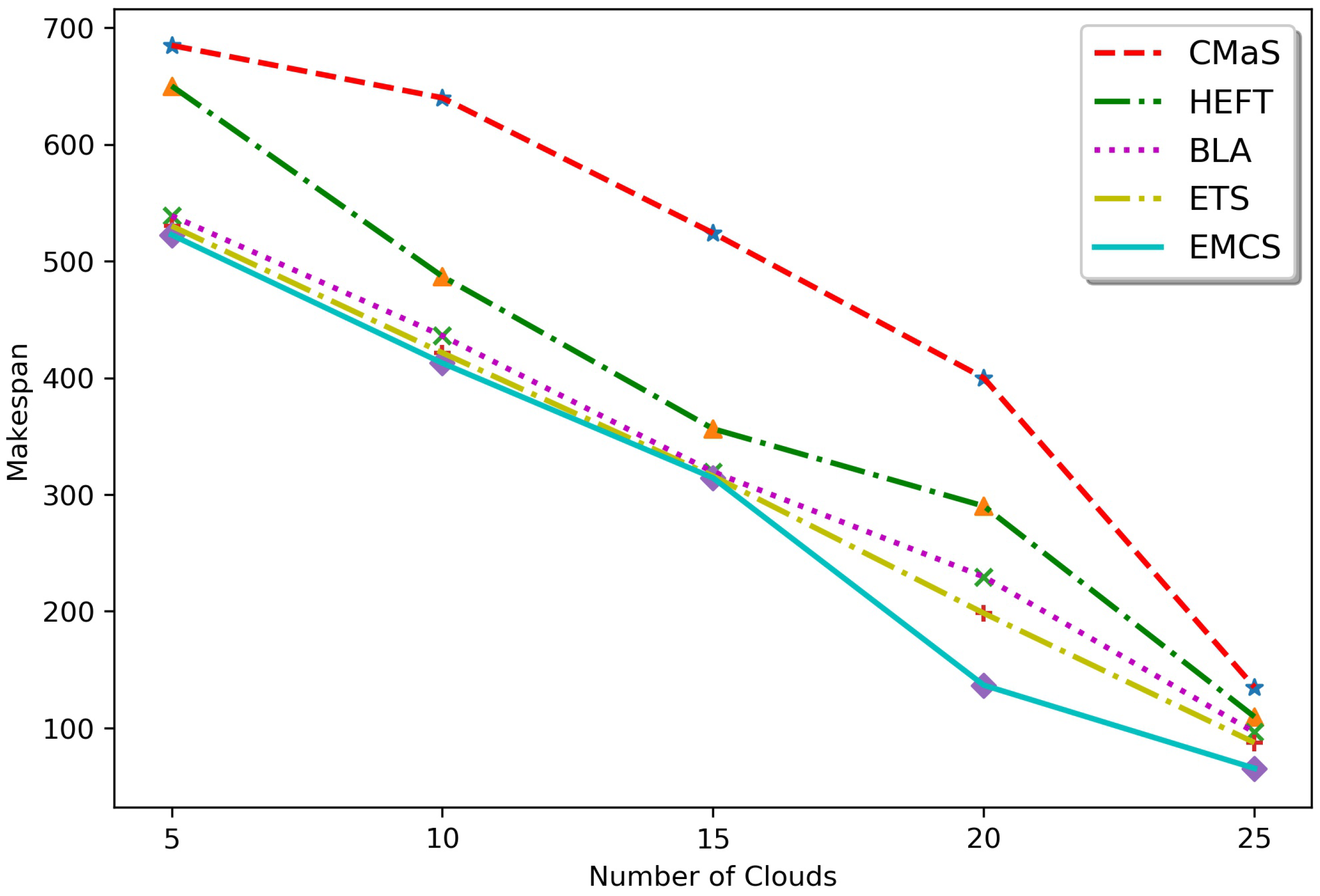
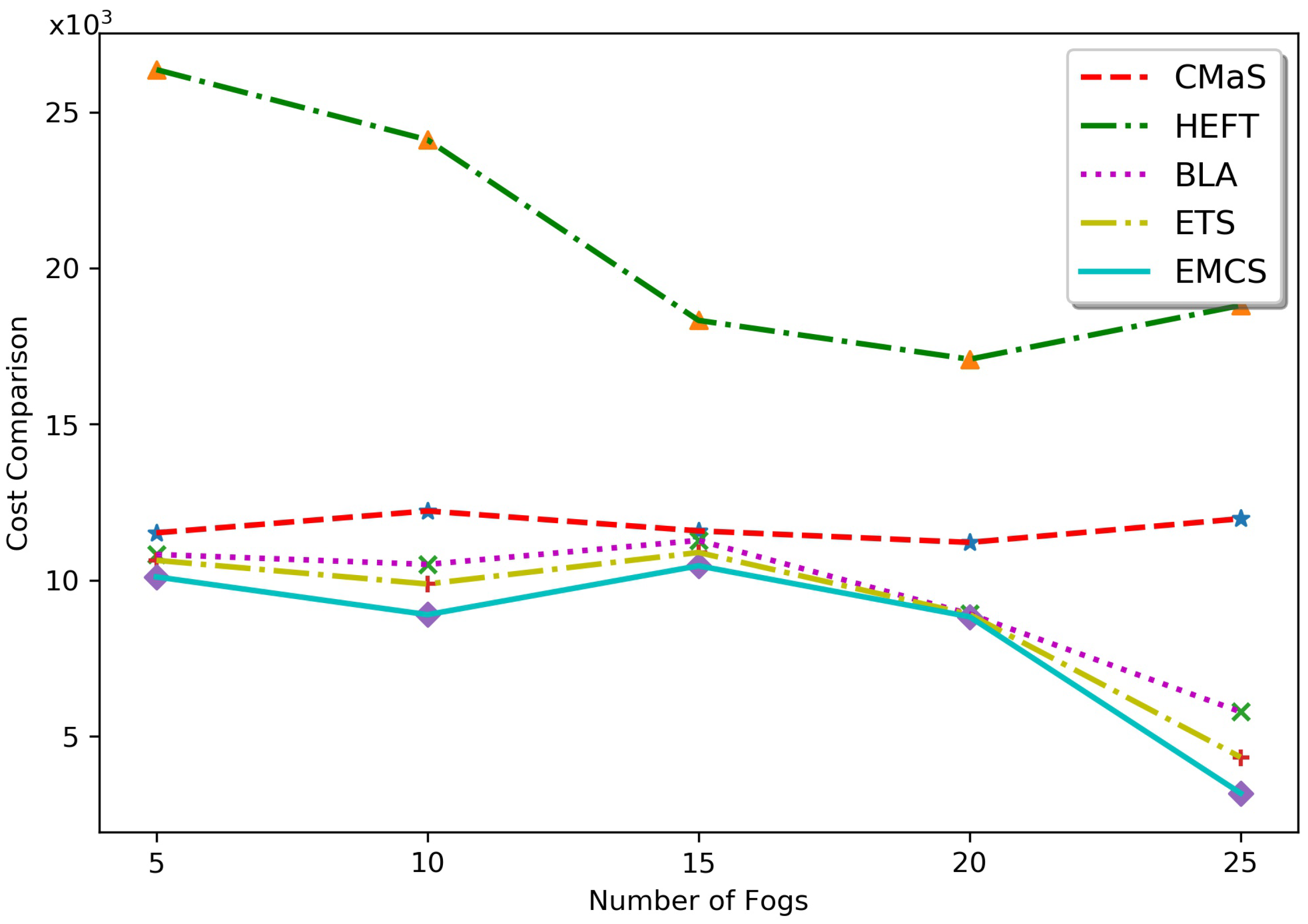
• The simulation results with various cloud and fog nodes also prove that the balance between cloud and fog nodes gives better performance.

The rest of the work is presented as follows. The study on task scheduling algorithms is discussed in Section 2. The system architecture and problem formulation are described in Section 2. The proposed EMCS task scheduling algorithm is elaborated in Section 4. Section 5 presents the performance of EMCS algorithm. Section 6 presents with conclusion and gives a future scope of the work.

2. Related Works

Many researchers have tried to distinguish between cloud and fog, and they also focused on the challenges and issues in fog computing. Advanced concepts such as MCC (mobile cloud computing), MEC (mobile edge computing), dew computing, edge computing, fog computing were examined by Naha et al. [5]. The architecture and research directions of fog computing are also focused on in this work. The basic model for networking, latency, and energy is discussed well in a survey presented by Mukherjee et al. [6]. The issues and challenges of application offloading, resource management, heterogeneity, and SDN (software-defined networking)-based fog computing are also described.

A major focus area of different network paradigms is the scheduling of tasks.

Table 1. Some related works on task scheduling in different systems.

Sl. No.	Article	Tar System	Ideas	Improved Criteria	Limitations
1	Pham et al. (2017) [1]	Cloud-Fog System	Utility function considering makespan and mandatory cost to prioritized tasks	Execution time and mandatory cost	Small dataset
2	Nguyen et al. (2019) [3]	Cloud-Fog System	Genetic algorithm	Makespan and total cost	Budget, deadline, and resource limitations are not considered
3	Bitam et al. (2018) [14]	Fog Computing	Bees Life algorithm	CPU execution time and memory allocation	Small dataset
4	Topcouglu et al. (2002) [13]	Heterogeneous Computing	Priority of tasks	Execution time	Complex network
5	Liu et al. (2018b) [16]	Fog Computing	Genetic algorithm	Makespan and communication cost	Based on the smart city database
6	Liu et al. (2018a) [17]	Fog Computing	Classification of mining	Execution time and waiting time	Bandwidth between processors is not considered
7	Xu et al. (2019) [18]	Cloud-Fog System	Laxity and ant colony optimization	Energy consumption	Small dataset
8	Benblidia et al. (2019) [19]	Cloud-Fog System	Fuzzy logic	Execution delay and energy consumption	Very small dataset
9	Boveiri et al. (2019) [21]	Cloud System	Max–Min ant system	Scheduling length	Small dataset and in the cloud environment
10	Aladwani (2019) [22]	Fog Computing	Max–Min system	Total execution time, total waiting time, and total finish time	Small dataset
11	Zhao et al. (2019) [20]	Cloud Computing	Greedy-based algorithm	Power consumption	Network optimization is not considered
12	Jena (2017) [23]	Cloud Computing	Clonal selection algorithm	Energy consumption and makespan	Data centers and jobs are dynamic
13	Alla et al. (2019) [24]	Cloud Computing	Best-worst and TOPSIS method	Makespan and energy consumption	Not used in the large-scale data center
14	Wang et al. (2019) [25]	Fog Computing	Hybrid heuristic algorithm based on IPSO and IACO	Delay and energy consumption	Only used for tasks generated from the smart production line
15	Rahbari and Nichkray (2018) [26]	Fog Computing	Knapsack-based symbiotic organism search	Energy consumption, total network usage, execution cost, and sensor lifetime	Implemented on tasks based on camera sensors with actuators
16	Wu and Lee (2018) [28]	Fog Computing	Heuristic algorithm on ILP model	Energy consumption	Two types of heterogeneous fog nodes
17	Kabirzadeh et al. (2018) [10]	Fog Computing	Hyper-heuristic algorithm selecting from GA, PSO, ACO, and SA	Energy consumption, network usage, cost	Limited to camera dataset
18	Tang et al. (2018) [29]	Mobile Cloud Computing	Greedy, Group and GA	Energy consumption	Small task graph and applied in MCC
19	Li et al. (2019) [30]	Cloud-Fog System	Nonlinear programming and STML approach	Energy consumption and delay	Fog nodes are homogeneous
20	Wu et al. (2021) [9]	Cloud-Fog System	Partition of graph with EDA	Energy consumption, makespan, and lifetime of IoT	Small but real-time data
21	Abdulredha et al. (2021) [15]	Cloud-Fog System	Evolutionary algorithm	Energy and makespan	Energy consumption is not considered

summarizes the models, policies and limitations of the task-scheduling algorithms. Some task-scheduling algorithms are discussed as follows. Pham et al. [1] considered DAG-based tasks with priorities. With the concept of the reassignment of tasks on the basis of a critical path for completing the execution before the deadline, a cost-makespan aware scheduling algorithm is developed. Nguyen et al. [3] applied an evolutionary strategy in TCaS (Time–Cost-aware Scheduling) algorithm for scheduling the Bag-of-Tasks in the cloud-fog model. Bitam et al. [14] proposed a new optimization method inspired by the natural life of bees called BLA, which is based on the population concept for collaborating the behaviors of bees, including marriage (reproduction) and food foraging. The initial population (N) is evaluated with the fitness function. The whole population is categorized as queen (best individual), drone (next D best individuals) and workers (remaining). Among the two phases of marriage and food forage, the queen mates with some drones in the marriage phase and produces broods by crossover and mutation operations. The best individual replaces the previous queen, and the next D fittest bees become drones and others are W workers. In the food forage, each individual is trying to search for food, and the workers collect the food. The best workers will remain in the next generation. This algorithm improves the CPU execution time and memory utilization of tasks. On the basis of rank for prioritizing the tasks, Topcouglu et al. [13] developed two algorithms: HEFT and CPOP (Critical-Path-on-a-Processor). Two processes, prioritization of task and selection of processors for the task execution, are considered in HEFT, whereas the critical path of the processors is considered in CPOP for minimizing the earliest finish time. Liu et al. [16] designed an Adaptive Doublefitness Genetic Task Scheduling algorithm that considers makespan and communication cost as doublefitness for scheduling tasks and fog resources. On the basis of the transaction set for scheduling and association rules of the nodes, the task set is generated, and using the association rules, the tasks are scheduled among the fog nodes. Based on this mining concept, the I-Apriori algorithm is developed by Liu et al. [17] for minimizing average waiting time and total excution time. Xu et al. [18] applied laxity for sequencing the priority of the task and applied ant colony optimization to reduce the energy consumption on satisfying mixed deadlines in hybrid cloud-fog computing. Benblidia et al. [19] ranked the fog nodes by considering the preferences of the users and fog nodes features, applying a linguistic quantifier and fuzzy quantified proposition. Zhang et al. [20] designed a delay optimal task scheduling (DOTS) algorithm which reduces the finish time. Boveiri et al. [21] adopted an approach of the Max–Min Ant system which solved a scheduling problem represented as a task graph in a multiprocessor system. Aladwani [22] developed a method called Tasks Classifications and Virtual Machines Categorization (TCVC) based on max–min scheduling applied to a health monitoring system and reduced the total finish time, execution time, and waiting time. Abdulredha et al. [15] used an evolutionary task-scheduling algorithm which can minimize the makespan and cost.

Here, we also studied some articles related to energy consumption in both cloud and fog systems. Using power-aware task scheduling, Zhao et al. [20] tried to predict the power consumption of a heterogeneous cloud platform. Jena [23] modeled a clonal selection-based algorithm (TSCSA) to utilize the resources effectively and reduce energy and execution time. Alla et al. [24] ranked each task based on a TOPSIS multi-criteria decision-making strategy. The ranked tasks are sent to the proper VM from dynamic priority queues through an energy-efficient dispatcher. It effectively reduces the makespan and energy consumption. Wang and Li [25] formed a hybrid heuristic algorithm adopting two algorithms, IPSO and IACO, in which delay and energy consumption are the main objectives for task scheduling. In [26], the tasks generated from camera sensors and actuators are scheduled with knapsack-based symbiotic organism scheduling that reduces energy and energy. Similarly, in [27], a greedy-based knapsack scheduling approach was followed for allocating resources in fog networks to improve energy consumption, execution cost, and delay. Wu and Lee [28] obtained the optimal scheduling strategy for energy minimization by solving the Integer Linear Programming model. A heuristic algorithm called Energy Minimization Scheduling (EMS) was proposed for reducing energy consumption. A hyper-heuristic technique of GA, PSO, ACO, and SA for current workflow is designed by Kabirzadeh et al. [10], which selects the best algorithm according to the lowest Euclidean distance. Three different heuristic algorithms (greedy based, group-based, and GA algorithms) are followed to schedule the tasks of mobile users on mobile cloud computing. This approach was proposed by Tang et al. [29], which reduces energy consumption by considering task dependency, transmission, task deadline, and cost. Li et al. [30] modeled an energy optimization algorithm considering energy consumption in each layer with nonlinear programming and delay optimization in STML (Scheduling to Minimize Lateness) approach. Wu et al. [9] adopted a partition operator to divide the graph into two non-overlapping sub-graphs. The proposed EDA (Estimation of Distributed Algorithm) has sorted the tasks for the fog and cloud layer according to their precedence. The permutation of tasks reduces the energy consumption and makespan along with a lifetime of IoT. Many such task-scheduling strategies on distributed systems can also be found in [31,32,33,34,35,36,37,38,39,40,41,42,43,44,45].

From the above works discussed, most of the papers considered the minimum completion of time and energy. In this paper, the consumption of energy for both fog and cloud are considered. The energy consumed in fog node is the energy usage for the processing of the tasks and energy required for an idle node. The energy consumed in the cloud node is the sum of the energy usage for processing and the energy usage for the transmission of the tasks and data to the cloud node. The evolutionary method is applied in the proposed approach for optimal makespan, cost, and energy consumption.

3. System Model

In this section, the network model, process flow model, problem formulation, earliest finish time model, cost model, and energy model of the system are clearly discussed.

3.1. Network Model

We assume a three-layer system. The first layer is the collection of IoT devices $\left\{i_1,i_2,\dots ,i_n\right\}$ that gather the data and send it to the immediate upper layer for further processing. The middle fog layer contains fog nodes $\left\{f_1,f_2,\dots ,f_m\right\}$ that can compute, store and communicate. The topmost cloud layer consists of high-performance servers $\left\{S_1,S_2,\dots ,S_n\right\}$ with enough storage and processing capability, as shown in Figure 1. Each Server $S_i$ consists of a set of virtual machines such as $\left\{V{M}_1,V{M}_2,\dots ,V{M}_k\right\}$. Each $VM$ is characterized by a processing rate and memory.

The data can transfer from cloud to fog and also from fog to cloud according to the request at the time of processing. The fog layer contains a $C{F}_{manager}$ (cloud fog manager) which gathers all the tasks and resources, and it runs a task scheduler. The task-scheduling scheme makes a decision regarding whether the task will be executed in the fog or cloud node; accordingly, the task is offloaded. The outcome of the task execution is sent back to the $C{F}_{manager}$. The $C{F}_{manager}$ integrates all the outcomes and sends it to the IoT devices. The EMCS task-scheduling algorithm is installed in $C{F}_{manager}$ for performing an optimal task execution schedule.

Table 2. Notations and description.

Sl. No.	Notation	Description
1	$i_n$	Represents IoT devices
2	$f_m$	Represents fog nodes
3	$S_n$	Represents cloud nodes
4	$C{F}_{manager}$	Cloud fog manager
5	$\left\{T_1,T_2,T_3,\dots ,T_n\right\}$	Set of tasks
6	$T_i$	Individual task where $iϵ\left[1,n\right]$
7	$T_{i-length}$	Number of instructions of task $T_i$
8	$\left\{P{N}_1,P{N}_2,P{N}_3,\dots ,P{N}_m\right\}$	Set of processors
9	$P{N}_i$	Individual processor where $iϵ\left[1,m\right]$
10	$P{N}_c$	Numerous cloud nodes
11	$P{N}_f$	Numerous fog nodes
12	$T_{entry}$	Entry task that does not have predecessors
13	$T_{exit}$	Exit task that does not have sucessors
14	$P{N}_{bw}\left[k\right]$	Bandwidth of processor k
15	$pred\_time\left[T_i\right]$	Time for completion of preceding tasks of $T_i$
16	$net\_In\left[T_i,P{N}_p\right]$	Total input to processor $P{N}_p$ for task $T_i$
17	$ES{T}_{P{N}_p}\left[T_i\right]$	Task $T_i^{\prime }s$ earliest start time on processor $P{N}_p$
18	$EF{T}_{P{N}_p}\left[T_i\right]$	Task $T_i^{\prime }s$ earliest finish time on processor $P{N}_p$
19	$avail\left(P{N}_p\right)$	Available of processor $P{N}_p$
20	$W_{P{N}_p}\left[T_i\right]$	Task $T_i^{\prime }s$ execution time on processor $P{N}_p$
21	$E_{P{N}_p}\left[T_i\right]$	Energy required to process task $T_i$ on processor $P{N}_p$
22	$E_{comm}^{P{N}_p}\left[T_i\right]$	Energy for communication of a task $T_i$ on processor $P{N}_p$
23	$c_1$	Processing cost per unit time for fog and cloud
24	$c_2$	Communication cost per unit time for fog and cloud
25	$e_f$	Energy required per unit for a execution of a task
26	$e_{idle}$	Energy used when fog is idle
27	$e_{comm}$	Energy per unit for transmission of data
28	$e_c$	Energy per unit for execution of the task in the cloud
29	$\alpha$,$\beta$,$\gamma$	Balance coefficient
30	$\epsilon$	Probability of crossover
31	$\mu$	Probability of mutation

show notations used in this paper.

3.2. Communication Model

The communication model followed in our system architecture is similar to [46]. It is a hybrid communication model which used both hierarchical and peer-to-peer (P2P) communication. The communication between the layers is hierarchical, and the communication between the nodes in the fog layer is P2P. The details of the communication mechanism in each layer are discussed below:

• IoT Device Layer: In this layer, the devices communicate with the fog nodes which are within the communication range using different wireless communicate protocols.
• Fog Layer: In this layer, the fog nodes communicate with each other using device-to-device (D2D) communication. All the fog nodes follow a uniform wireless communication protocol.
• Cloud layer: This layer consists of multiple cloud servers which are kept in a centralized data center. The servers are connected through wired links for communication. The communication pattern followed between the cloud and fog layer is wireless in nature.

The process flow model below shows the whole process of the task-scheduling algorithm.

3.3. Process Flow Model

This section discusses the task-scheduling process that will occur in the three-layered architecture. The steps are presented below and shown in Figure 2.

• Step 1: The IoT devices collect the data and send a request to the closest fog node.
• Step 2: The fog node immediately transfers the request to the $C{F}_{manager}$.
• Step 3: To process a request, the request is decomposed into numerous dependent tasks which can be executed in the processors.
• Step 4: Then, the resource usages and the number of instructions of a task are estimated.
• Step 5: The task scheduler runs a scheduling algorithm and finds an optimal scheduling scheme.
• Step 6: As a result of the scheduling algorithm, the task are offloaded to the corresponding cloud and fog nodes.
• Step 7: The task collects the data from preceding tasks which completed their processes either in cloud node or fog node.
• Step 8: Each task is executed in the corresponding node.
• Step 9: After task execution was completed, the results are returned to the $C{F}_{manager}$.
• Step 10: After the completion of all tasks, the results of a request are combined by the $C{F}_{manager}$.
• Step 11: The aggregated result is bundled as a response and sent to the IoT device through the fog node.

Using the above models, the assumptions considered in this proposed work are discussed as follows. (a) The IoT devices send the job requests to the nearest fog node. (b) A job request consists of a set of dependent tasks. (c) The dependent tasks of a single job request are scheduled to multiple fog/cloud nodes. (d) The tasks are both memory and CPU intensive. (e) Due to task dependency, whenever there is a requirement of data transfer from one fog node to another, the sender fog node transfers the data to the nearest fog node. (f) The fog nodes have the same communication bandwidth due to there being a uniform communication model as described above. (g) The heterogeneity lies in fog only in terms of processing capacity and energy consumption per unit time for the execution of a task. (h) The servers have different communication bandwidths in the data center.

3.4. Problem Formulation

Consider the request which is decomposed with numerous dependent tasks in $C{F}_{manager}$ and represented on a DAG. The dependent task set is T=$\left\{T_1,T_2,T_3,\dots \dots ,T_n\right\},$ and each task $T_i$ contains $T_i=\left\{Ti{d}_i,dsiz{e}_i,T_{(i-length)}\right\}$, where $Ti{d}_i$, $dsiz{e}_i$,$T_{(i-length)}$ represents the task identification number, the required data from other processors, and number of instructions. These tasks are assigned to the DAG, which is represented as $G=(T,C)$ where T = $\left\{T_1,T_2,\dots ,T_n\right\}$ ($\forall T_iϵT,iϵ\left[1,n\right]$), and C represents the edge where $C_{ji}ϵC(T_i,T_jϵT)$ shows that after the completion of task $T_j$, task $T_i$ will start. The weight of $C_{ji}$ shows the data size transferred from task $T_j$ to $T_i$ and $dsiz{e}_i=\sum C_{ji}$. The predecessor and the successor of $T_i$ are denoted as $pred\left(T_i\right)$ and $succ\left(T_i\right)$, respectively. The entry task does not have a predecessor, and the exit task does not have a successor. Thus, the entry task and exit task can be represented as $T_{entry}$ and $T_{exit}$, respectively.

The processors of the cloud-fog network can also be represented with a complete graph $G=(PN,E)$ where $PN$ = $\left\{P{N}_1,P{N}_2,..,P{N}_m\right\}$ ($\forall P{N}_iϵPN,iϵ\left[1,m\right]$) denotes the processor set and $E_{ij}ϵE$ is the link between $P{N}_i$ and $P{N}_j$.

Let $P{N}_c$ represent the numerous cloud nodes and $P{N}_f$ represent the numerous fog nodes. Then, the total nodes can be represented as $PN=P{N}_c\cup P{N}_f$. The processing rate and bandwidth of a processor can be denoted as $P{N}_{pr}\left[p\right]$ and $P{N}_{bw}\left[p\right]$, where $p=\left\{1,2,\dots ,m\right\}$, respectively. All the cloud and fog processors are heterogenous and have different processing rates. The cloud nodes have different bandwidths, but as the fog nodes are far from the cloud and placed in one layer, the bandwidth of the fog node is considered as same. It is assumed that when a task is offloaded to the cloud, it starts its execution immediately without waiting in a queue.

Figure 3 shows both the task and processor graph, where we consider eight dependent tasks $\left\{T_1,T_2,\dots ,T_8\right\}$ represented in DAG and four processors $\left\{P{N}_1,P{N}_2,\dots ,P{N}_4\right\}$ represented in a complete graph. The tasks $T_2$, $T_3$ and $T_4$ cannot be processed until task $T_1$ is completed its execution. Similarly, task $T_5$ will start execution after the completion of tasks $T_2$ and $T_3$, task $T_6$ will start after the completion of tasks $T_3$ and $T_4$, task $T_7$ will start after the completion of tasks $T_3$, $T_4$ and $T_5$ and finally, $T_8$ will start execution after the completion of tasks $T_6$ and $T_7$. The outcomes of predecessor tasks will be the input of the consequent task. The tasks have priority that the task will start its execution only if the input resources of the task are available. The input resources are not only the outcomes of predecessor tasks but also the data from either cloud or fog nodes. The major objective is the assignment of tasks to the processors in such a way that the system has optimum completion time, reduced cost, and energy consumption. Here, our task scheduler schedules the tasks on the processors considering all these criteria.

Theorem 1. 

The proposed EMCS algorithm is intractable.

Proof. 

The proposed EMCS algorithm considers a task set $T=\left\{T_1,T_2,T_3,\dots \dots ,T_n\right\}$. Each $T_i$ has a number of instructions $T_{i-length}$. $PN=\left\{P{N}_1,P{N}_2,\dots ,P{N}_m\right\}$ are the number of processors of cloud-fog network. The processing rate and bandwidth of processor $P{N}_i$ are $P{N}_{pr}\left[i\right]$ and $P{N}_{bw}\left[i\right]$, respectively. The problem is to assign task $T_i$ to processor $N_j$ after completion of the execution of a task at processor $N_j$. As the tasks are dependent, after the completion of a task, the successor task will be started. There are $m^n$ possible solutions to map tasks to processors, which is a challenging task. In real time, m and n are very large in terms of thousands. This problem can be reduced to a bin-packing problem where processors $N=\left\{N_1,N_2,..,N_m\right\}$ can be mapped to bins $k=\left\{k_1,k_2,\dots ,k_m\right\}$ and tasks $T=\left\{T_1,T_2,T_3,\dots \dots ,T_n\right\}$ can be mapped to objects $S=\left\{s_1,s_2,s_3,\dots \dots ,s_n\right\}$. Here, $T_{i-length}$ is mapped to volume $V_i$[47]. The bin-packing problem is an NP-hard problem; hence, our proposed EMCS algorithm is also NP-hard.    □

3.5. Earliest Finish Time Model

In this section, we have shown the makespan model of the proposed task-scheduling algorithm. Following Pham et al. [1], the task $T_i$ can start its execution after the completion of all preceding tasks of $T_i$ on processor $P{N}_p$ and also after obtaining all the input data from the other nodes. The time for completion of preceding tasks can be defined as:

$$pred\_time\left[T_i\right]=\underset{T_jϵpred\left(T_i\right),P{N}_qϵPN}{max}\left[EFT(T_j,P{N}_q)\right]$$

(1)

$EFT(T_j,P{N}_q)$ is the earliest finish time of task $T_j$ on processor $N_q$. For the entry task, $pred\_time\left[T_{entry}\right]=0$. When $T_i$ executes in $P{N}_p$, the input data of $T_i$ are the outcomes of the predecessor task, and the data from the cloud or fog nodes must be available as well. If $net\_In[T_i,P{N}_p]$ is the total input data of task $T_i$ required for processing the task in processor $P{N}_p$, then it can be represented as:

$$net\_In\left[T_i,P{N}_p\right]=\left\{\begin{array}{cc}\left(dt\left[T_i,P{N}_q\right]+\sum _{T_jϵpred\left(T_i\right)}^{T_jϵP{N}_q}{C}_{qp}\right)\times \left(\frac{1}{P{N}_{bw}\left[p\right]}+\frac{1}{P{N}_{bw}\left[q\right]}\right)\hfill & \mathrm{if}P{N}_p\ne P{N}_q\hfill \\ 0\hfill & \mathrm{if}P{N}_p=P{N}_q\hfill \end{array}\right.$$

(2)

where $dt[T_i,P{N}_q]$ is the size of the data, which is required to transfer from processor $P{N}_q$ for executing task $T_i$. The earliest start time $ES{T}_{P{N}_p}\left[T_i\right]$ and earliest finish time $EF{T}_{P{N}_p}\left[T_i\right]$ of task $T_i$ on processor $P{N}_p$ are computed as:

$$ES{T}_{P{N}_p}\left[T_i\right]=max\left\{avail\left(P{N}_p\right),pred\_time\left[T_i\right]+max\left(net\_In\right)\right\}$$

(3)

$$EF{T}_{P{N}_p}\left[T_i\right]=W_{P{N}_p}\left[T_i\right]+ES{T}_{P{N}_p}\left[T_i\right]$$

(4)

where $avail\left(P{N}_p\right)$ is the availability of processor $P{N}_p$ for executing task $T_i$ and $W_{P{N}_p}\left[T_i\right]$ is the execution duration of task $T_i$ on node $P{N}_p$, and these are represented as:

$$avail\left(P{N}_p\right)=\underset{T_jϵP{N}_p}{max}\left[EF{T}_{P{N}_p}\left[T_j\right]\right]$$

(5)

$$W_{P{N}_p}\left[T_i\right]=\frac{T_{i-length}}{P{N}_{pr}\left[p\right]}$$

(6)

The time of completion of all the tasks ($makespan$) is the earliest finish time of the last task $T_{exit}$, which can be calculated as the $EF{T}_{P{N}_p}\left[T_{exit}\right]$. So,

$$makespan=EF{T}_{P{N}_p}\left[T_{exit}\right]$$

(7)

3.6. Cost Model

The cloud charges a monetary cost for processing a task which includes processing cost along with communication cost, while a fog node demands only communication cost [1]. The communication cost for both cloud and fog node is the total cost for transferring data from the predecessor node as well as the cost for transferring data from other cloud or fog nodes. Hence, the monetary cost $Cos{t}_{P{N}_p}\left[T_i\right]$ for executing task $T_i$ on $P{N}_p$ can be computed as:

$$Cos{t}_{P{N}_p}\left[T_i\right]=\left\{\begin{array}{cc}{c}_1\times W_{P{N}_p}\left[T_i\right]+c_2\times \sum _{P{N}_pϵP{N}_c}^{}\left(dt\left[T_i,P{N}_p\right]+\sum _{T_jϵpred\left(T_i\right)}^{T_jϵP{N}_q}{C}_{qp}\right)\hfill & \mathrm{if}P{N}_pϵP{N}_c\hfill \\ c_2\times \sum _{P{N}_pϵP{N}_c}^{}\left(dt\left[T_i,P{N}_p\right]+\sum _{T_jϵpred\left(T_i\right)}^{T_jϵP{N}_q}{C}_{qp}\right)\hfill & \mathrm{if}P{N}_pϵP{N}_f\hfill \end{array}\right.$$

(8)

where $c_1$ is the processing cost per unit time and $c_2$ is the cost for transferring the data to processor $P{N}_p$ for executing the task $T_i$.

The total cost can be calculated as:    

$$Total\_cost=\sum _{T_iϵT,P{N}_pϵPN}^{}Cos{t}_{P{N}_p}\left[T_i\right]$$

(9)

3.7. Energy Model

If $T_i$ is assigned to a fog node $P{N}_p$, the energy usage in the fog node can be estimated as energy required for executing the task and energy usage when the fog node is being idle [48]. The IoT devices communicate with the fog nodes which are within the communication range of them. The communication among fog nodes follows a D2D pattern where a sender fog node transfers data to the nearest fog node. Due to the close proximity transmission between the fog nodes, the communication energy is negligible. When $P{N}_p$ is the cloud node, the energy consumption is considered as the sum of energy usage for execution of a task and the transmission of both task and data. The energy for the transmission of task and data can be represented as communication energy consumption $E_{comm}^{P{N}_p}\left[T_i\right]$. The energy required to execute a task in a node is as follows:

$$E_{P{N}_p}\left[T_i\right]=\left\{\begin{array}{cc}{e}_f\times W_{P{N}_p}\left[T_i\right]+e_{idle}\hfill & \mathrm{if}P{N}_pϵP{N}_f\hfill \\ e_f\times W_{P{N}_p}\left[T_i\right]+E_{comm}^{P{N}_p}\left[T_i\right]\hfill & \mathrm{if}P{N}_pϵP{N}_{c}andp\ne q\hfill \end{array}\right.$$

(10)

where

$$E_{comm}^{P{N}_p}\left[T_i\right]=e_{comm}\times \left\{\left(dt\left[T_i,P{N}_p\right]+\sum _{T_jϵpred\left(T_i\right)}^{T_jϵP{N}_q}{C}_{qp}\right)+T_{i-length}\right\}$$

(11)

where $e_f$ is the energy per unit for executing a task in a fog node, $e_{idle}$ is the energy used when a fog node is being idle, $e_{comm}$ is the energy per unit for the transmission of data from other nodes to the cloud node, and $e_c$ is the energy per unit used to process a task in the cloud.

The total energy consumption is calculated as follows:

$$E=\sum _{P{N}_pϵPN,T_iϵT}^{}{E}_{P{N}_p}\left[T_i\right]$$

(12)

Theorem 2. 

Energy consumption of a processor in cloud_fog network is $E_{P{N}_p}\left[T_i\right]$.

Proof. 

The fog as well as the cloud node energy consumption are considered to prove the lemma. The fog node is used for executing a task or it will be in idle mode. The fog nodes are closed to the IoT devices and the data one fog node is transmitted to the nearest fog node; thus, the transmission energy consumption is negligible. Hence, the amount of energy consumed to process a task $T_i$ in fog node $P{N}_f$ is represented as:

$$E_{P{N}_f}\left[T_i\right]=e_f\times W_{P{N}_f}\left[T_i\right]+e_{idle}$$

(13)

where $e_f$ is the energy per unit time for executing a task in the fog node, and $e_{idle}$ is the energy used when the fog node is idle. In case of a cloud node, the energy consumption for the execution and transmission of data is considered where the idle time is ignored. So, the amount of energy consumed to process a task $T_i$ in cloud node $N_c$ is

$$E_{P{N}_c}\left[T_i\right]=e_c\times W_{P{N}_c}\left[T_i\right]+e_{comm}^{P{N}_c}\left[T_i\right]$$

(14)

where $e_c$ is the energy per unit used to process a task in the cloud. If $N_c$ is the processor to process a task $T_i$, the energy consumption formulation can be calculated as shown in Equation (10), where $P{N}_p=P{N}_c$.    □

Theorem 3. 

Transmission energy consumption for a task $T_i$ to execute in a cloud node $P{N}_c$ is $e_{comm}^{P{N}_p}\left[T_i\right]$.

Proof. 

If the task $T_i$ will be executed in a cloud node, then the amount of data transferred from IoT device to cloud node is $T_{i-length}$. When a task is executed in a cloud node, it collects the link data from the other processors, which is represented in Equation (2) as:

$$\left(dt\left[T_i,P{N}_p\right]+\sum _{T_jϵpred\left(T_i\right)}^{T_jϵP{N}_q}{C}_{qp}\right)$$

(15)

where $P{N}_p$ is the cloud node and $P{N}_q$ is another processor. Thus, the energy required for the transmission of a task $T_i$ to a cloud node is calculated and represented in Equation (11).    □

4. Proposed EMCS Task Scheduling Algorithm

In this work, the EMCS algorithm is proposed which uses the GA evolutionary strategy. The proposed method optimizes the task completion time, cost and energy consumption. EMCS learns from biological reproduction such as selection, crossover, mutation, and finding the best individual. The steps are shown below and the algortihms for these processes are presented in Algorithms 1 and 2.

Algorithm 1 Algorithm for fitness value computation

Input: DAG of task, chromosome, location Output: fitness value 1: $sorted\_task\leftarrow topological\_sort\left(task\right)$ 2: for$T_i$ in $sorted\_task$ do 3:     $P{N}_p\leftarrow chromosome\left[T_i\right]$ 4:     if $T_i==T_{entry}$ then 5:          $pred\_time\left[T_i\right]\leftarrow 0$ 6:     else 7:          Compute $pred\_time\left[T_i\right]$ 8:     end if 9:     for $T_j$ in predecessors($T_i$) do 10:          $P{N}_q\leftarrow chromosome\left[T_j\right]$ 11:          if $T_j==Null$ then 12:              $net\_In[T_i,P{N}_p]\leftarrow 0$ 13:          else if $P{N}_p\ne P{N}_q$ then 14:              Compute $net\_In[T_i,P{N}_p]$ 15:          end if 16:     end for 17:     Compute $EST\left[T_i\right]$, $EFT\left[T_i\right]$, $Cost\left[T_i\right]$, $E\left[T_i\right]$ 18: end for 19: Set $\alpha$,$\beta$,$\gamma$; 20: Compute utility function F; 21: Return F;

Algorithm 2 Algorithm for best solution selection

Input: Fitness value, chromosome, location Output: best_solution (chromosome, fitness, pop_location) 1: Set $fitness\_function\leftarrow Fitnessvalue$ 2: Set $population\_size$ and $num\_generation$ 3: for$n\leftarrow 1$ to $num\_generation$ do 4:      use roulette wheel selection to select chromosomes 5:      use two-point crossover with probability $ϵ$ 6:      use mutation with probability $\mu$ 7: end for 8: Return $best\_solution$

4.1. Chromosome Encoding

The chromosome is encoded by assigning a processor to the task. Each individual chromosome is the outcome of the task scheduling. The chromosome can be encoded as n-bits with values ranging from [1:m], where m is the total processors and n is the total tasks. The processors are both cloud and fog nodes. If 1 to k are the cloud nodes, then $k+1$ to m are the fog nodes. The task is represented as the index of the chromosomes, and the chromosome represents the assigning of the processors (i.e., both cloud and fog nodes) to the tasks. As shown in Figure 4, the number of tasks and processors are 8 and 4. The processors 1 and 2 are the cloud nodes and processors 3 and 4 are the fog nodes, respectively. The number of tasks decides the length of the chromosome, which is 8 bits in this scenario. Thus, the chromosome can be represented as follows:

The chromosome <3, 4, 1, 3, 1, 3, 4, 2> means processor 3 executes tasks 1, 4 and 6, processor 4 executes tasks 2 and 7, processor 1 executes tasks 3 and 5, and similarly, processor 2 executes task 8.

This type of chromosome encoding was chosen for a better performance of genetic operations (crossover and mutation) to create new offspring by inheriting quality genes from parents in the solution search space. The order of execution of the tasks is to be considered because the task can be processed after the completion of the dependent task.

4.2. Population Initialization

All possible chromosomes belong to the solution search space. The population can be initialized by choosing a set of chromosomes randomly. Let N be the size of the population, then N number of chromosomes are randomly selected from the solution search space, ensuring the diversity of the first-generation population. Some operations are applied to the selected individuals of the initial population to create offsprings.

4.3. Fitness Function

The quality of the individual can be determined by the fitness function. The individuals with maximum fitness value are considered as quality outcomes. The fitness value can be determined for each individual by maximizing the utility function F calculated below:

$$F=\alpha \times \frac{min\left(EF{T}_{P{N}_p}\right)}{makespan}+\beta \times \frac{min\left(Cos{t}_{P{N}_p}\right)}{Total\_Cost}+\gamma \times \frac{min\left(E_{P{N}_p}\right)}{E}$$

(16)

where $\alpha$, $\beta$, and $\gamma$ are the balanced coefficients such that the sum of them is 1. The values of $\alpha$, $\beta$, and $\gamma$ are considered according to the priority of the makespan, cost or energy consumption. If we give high priority to minimize the makespan, then $\alpha$ is considered with value in range 0.5–1 and other two $\beta$, and $\gamma$ are considered in between 0.5–1. Similarly, if minimization of cost is high priority then $\beta$ value is set in the range of 0.5–1 and $\alpha$ and $\gamma$ are considered in the range of 0.5–1. This way $\gamma$ is also considered in the range of 0.5–1, while the minimization of energy consumption is considered for higher priority, and the other two are in the range of 0.5–1. Algorithm 1 presents the whole steps for fitness value calculation.

4.4. Genetic Operators

Here, the genetic operators are selection, crossover, and mutation. The selection operator selects the populations with higher fitness values. The crossover recombines the genes to inherit the best gene to the next generation. The mutation maintains the diversity from one generation to the next generation.

• Crossover: The crossover generates new individuals by crossing the genes of two individuals of the population. In this work, the traditional two-point crossover is applied to the parents for inheriting the quality genes in offspring. The process is shown in Figure 5, where two points are selected randomly and the genes between these two points of the first and second parents are exchanged with each other, while the remaining genes are unchanged to generate new offspring.
  The selection of parents in the crossover process can influence the algorithm. The crossover rate of every individual is $\epsilon$. The parents are selected for crossover by applying a roulette wheel process. From this technique, the best individual with a maximum fitness value has a chance to be the parent, ensuring the offspring have good genes.
• Selection Process: The selection process selects a set of individuals on the basis of Darwin’s law of survival and forms a population for the next generation. After the crossover operation, the fitness value of the offspring is calculated. Here, 40% of parents are selected for the next generation, and the remaining population will be formed with offspring of the highest fitness value. Other individuals are discarded in this process. In this selection process, individuals with lesser fitness values are not discarded rapidly, and they are used to explore the search area, so that the population deviance is maintained in each generation.
• Mutation Operator: N chromosomes are formed with a new population after the completion of crossover and selection operations. Each individual with mutation rate $\mu$ has participated in a one-point mutation process. A random gene of each individual as shown in Figure 6 is selected, and the value of that gene is changed to a different value ranging from [1:m], which assigns the chosen task to be executed in another processor.
  The mutation overcomes the limitations of crossover by exploring the other areas in the solution space and avoiding local solutions. A set of modifications in GA was introduced in the proposed EMCS algorithm. Those are as follows:

  -

  Parent Selection: 75% of the population are selected as parents for crossover operations. This selection process adopts the roulette wheel technique of selecting parents for mating.

  -

  Selection Strategy: After crossover, 40% of parents are preserved for the next generation, and the remaining population is selected with offspring of larger fitness.

Algorithm 1 presents the fitness value calculation, which is discussed as follows. In this process, the task graph is considered as DAG, so that the topological sort function can be used to find dependencies, which is assigned to the $sorted\_task$ in step 1. Afterwards, we compute the following steps for each node $T_i$ of the $sorted\_task$:

• In step 3, assign processor $N_p$ with $chromosome\left[T_i\right]$ (i.e. selected processor for processing task $T_i$);
• In steps 4–7, check whether $T_i$ is the entry task or not. If $T_i$ is an entry task, then the set time for completion of the preceding tasks $pred\_time\left[T_i\right]$ is 0; otherwise, compute $pred\_time\left[T_i\right]$ using Equation (2). For each node $T_j$ of $predecessors\left(T_i\right)$, compute steps 9–15.
• In step 9, set $P{N}_q$ with $chromosome\left[T_j\right]$.
• In steps 10–15, check $P{N}_p\ne P{N}_q$; if true, then compute data transferring time from node $P{N}_q$ to node $P{N}_p$$net\_In[T_i,P{N}_p]$ using Equation (2); otherwise, set $net\_In[T_i,P{N}_p]$ as 0.
• In step 17, compute $EST\left[T_i\right]$, $EFT\left[T_i\right]$, $cost\left[T_i\right]$, and $E\left[T_i\right]$ using Equations (3)–(6), (8), (10) and (11). In step 19, set $\alpha$,$\beta$,$\gamma$ in such a way that $\alpha$+$\beta$+$\gamma =1$. In step 20, compute the utility function F using Equations (7), (9), (12) and (13). Finally, return F in step 21.

The time complexity of Algorithm 1 is the total time required to process the algorithm. The DAG $G=(T,C)$ is the set of task as the input. The total time complexity is calculated as follows.

• Step 1 requires $O(T+C)$ times for topological sort.
• The time required for executing step 2 to step 18 is $O(T\ast indeg(T\left)\right)$, where $indeg\left(\right)$ is the number of incoming edges to a node T.
• The time complexity of step 19 is 1.
• Similarly, the complexity of each step 20 and step 21 is 1.

The overall time complexity of the algorithm is $O(T+C)+O(T\ast indeg(T)+1+1+1=O(C+T\ast indeg\left(T\right))$.

Algorithm 2 presents the best solution selection. In step 1, a fitness function is assigned with a fitness value computed in Algorithm 1. Then, we set the population size and number of generations in step 2. Afterwards, repeat steps 4–6 for each generation. In these steps, perform roulette wheel selection, two-point crossover with probability, and mutation with probability for each generation. At last, return the best solution. The time complexity analysis of Algorithm 2 is shown as follows.

• Step 1 and step 2 has a time complexity of 1.
• Step 3 to step 7 has a time complexity of $O(num\_generation(population\_size+population\_size\ast chromosome\_size+population\_size\ast chromosome\_size)$.
• Step 8 has a time complexity of 1.

So, the overall time complexity of the algorithm is $1+1+O(num\_generation(population$

$\_size+population\_size\ast chromosome\_size+population\_size\ast chromosome\_size)+1=O(num\_generation\ast population\_size\ast chromosome\_size)$.

The whole process of Algorithms 1 and 2 for EMCS is shown in the flowchart in Figure 7.

5. Performance Evaluation

This section presents the experimental setup and evaluation of our proposed EMCS algorithm by comparing it with some other recent algorithms.

5.1. Experimental Setup

The experiments are conducted using the Python environment. The software or hardware taken for this simulation is shown in

Table 3. Hardware/Software Specification.

Sl. No.	Hardware/Software	Configuration
1	System	Intel® Core ™ i5-4590 CPU @ 3.30 GHz
2	Memory (RAM)	4 GB
3	Operating System	Windows 8.1 Pro

. The assumptions considered for implementing the algorithm are explained below.

Both cloud and fog nodes with different processing rates, monetary costs, and energy rates are considered. Each node has its own processing rate (represented by MIPS (million instructions per second)) as well as communication cost. The fog nodes have a minimal processing speed, while the cloud nodes have servers and virtual machines with high processing speed, which demands processing cost on the usage of the processors. The bandwidth of the fog nodes is higher than the cloud nodes. As all the fog nodes are placed in a middle layer, the bandwidth is the same for all fog nodes, and as per the heterogeneous behavior of the cloud, the bandwidth is varied. Similarly, the energy cost is more in cloud nodes compared to the fog nodes. The idle fog nodes have also consumed energy. Both cloud and fog nodes consume energy at the time of computation, and additional energy for communication is also consumed by the cloud. The cost is represented as Grid Dollar (G$), which is a currency unit used in this simulation.

In our model, we are considering a DAG for task graphs with varying sizes in MIPS. The task graph is randomly generated with different sizes from 20 to 100 with a complete graph of processors having a different set of fog and cloud nodes. The input and output files of a task have size from 10 to 50 MB. The performance of EMCS is evaluated by taking the parameters shown in

Table 4. Simulation parameters and values setup.

Sl. No.	Parameter	Value
1	Tasks	$[20,100]$
2	Cloud nodes ($P{N}_c$)	$[5,45]$
3	Fog nodes ($P{N}_f$)	$[5,45]$
4	Processing rate of cloud ($P{N}_{pr}$)	$[250,500]$ MIPS
5	Processing rate of fog ($P{N}_{pr}$)	$[10,500]$ MIPS
6	Bandwidth of cloud ($P{N}_{bw}$)	10, 100, 512, 1024 Mbps
7	Bandwidth of fog ($P{N}_{bw}$)	1024 Mbps
8	Amount of communication data ($dt[T_i,P{N}_p]$)	$[10,50]$ MB
9	Processing cost per time unit for cloud ($c_1$)	0.5 G$/s
10	Processing cost per time unit for fog ($c_1$)	$[0.1,0.5]$ G$/s
11	Communication cost per time unit for cloud ($c_2$)	$0.7G$$/s
12	Communication cost per time unit for fog ($c_2$)	$[0.3,0.7]$ G$/s
13	Number of instructions ($T_{(i-length)}$)	$[100,500]$${10}^9$ Instructions
14	Energy per unit time for execution of the task in fog ($e_f$)	$[1,5]$ w
15	Energy used when fog node is idle ($e_{idle}$)	0.05 w
16	Energy per unit for transmission of data ($E_{comm}$)	$[0.1,2]$ w
17	Energy per unit for execution of task cloud ($e_c$)	$[5,10]$ w
18	Balance coefficient ($\alpha ,\beta ,\gamma$)	$[0,1]$ and $\alpha +\beta +\gamma =1$

.

The evolutionary model is used in our algorithm. The values considered for the parameters of the GA are shown in

Table 5. Parameters of GA, BLA and ETS.

Name	GA	ETS	BLA
Length of chromosome	$[20,100]$	$[20,100]$	$[20,100]$
Number of iterations	100	100	100
Probability of crossover ($ϵ$)	0.9	0.9	0.9
Probability of mutation ($\mu$)	0.1	0.1	0.1
Population size	100	100	Q = 1 D = 30 W= 69

. The two-point crossover and single-point random mutation are considered.

For evaluating the performance of our model EMCS, the model is compared with other models such as CMaS [1], HEFT [13], BLA [14] and ETS [15]. CMaS is used to check the makespan and monetary cost, whereas HEFT is used only for makespan check. BLA is another evolutionary algorithm that checks the cost for execution and use of memory for allocating the tasks in the fog nodes. ETS is also an evolutionary algorithm that checks the makespan and cost for execution. For comparing the makespan, cost and energy consumption of all the models, the models are implemented with given parameter values. The values for parameters of BLA and ETS are shown in Table 5.

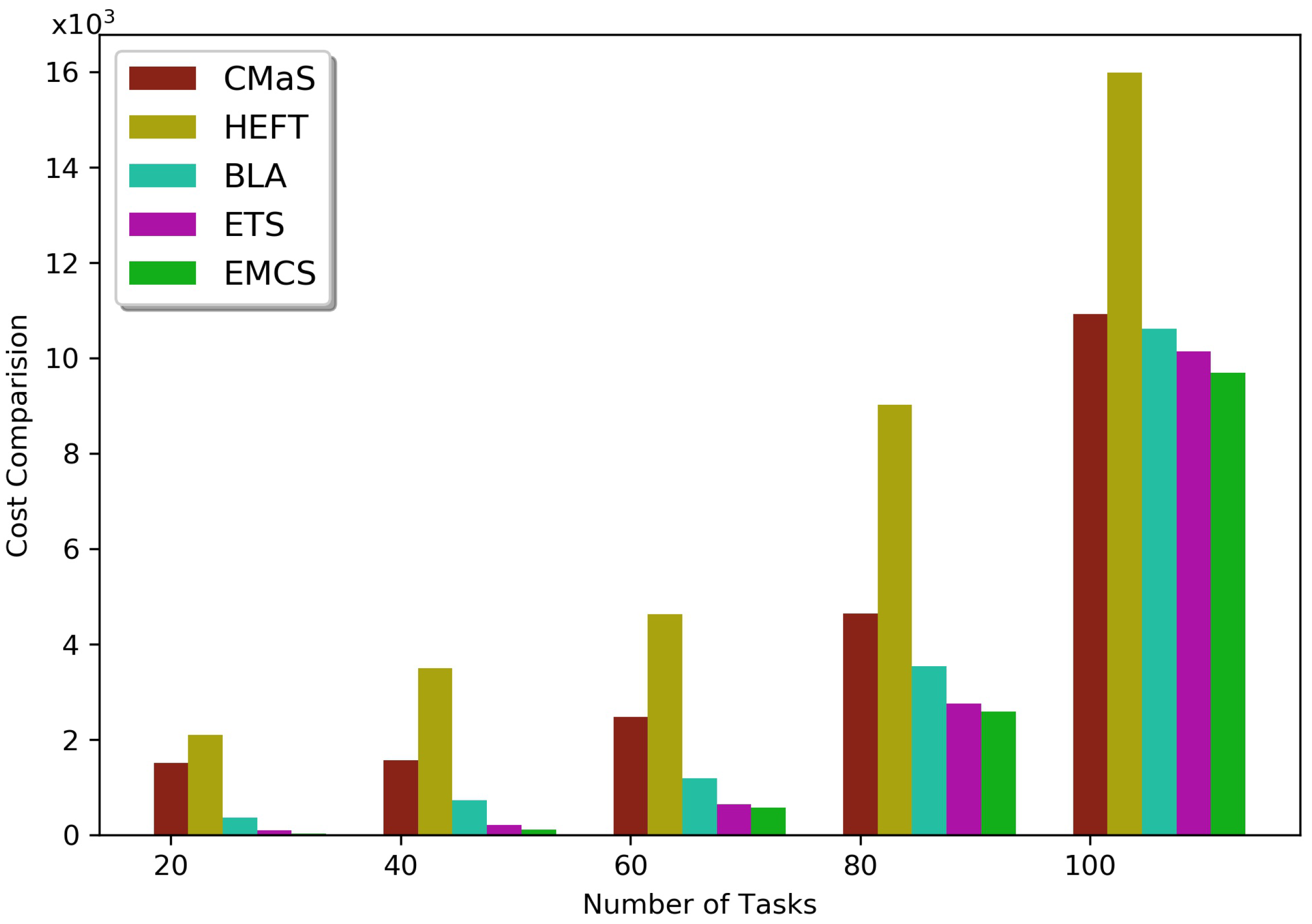
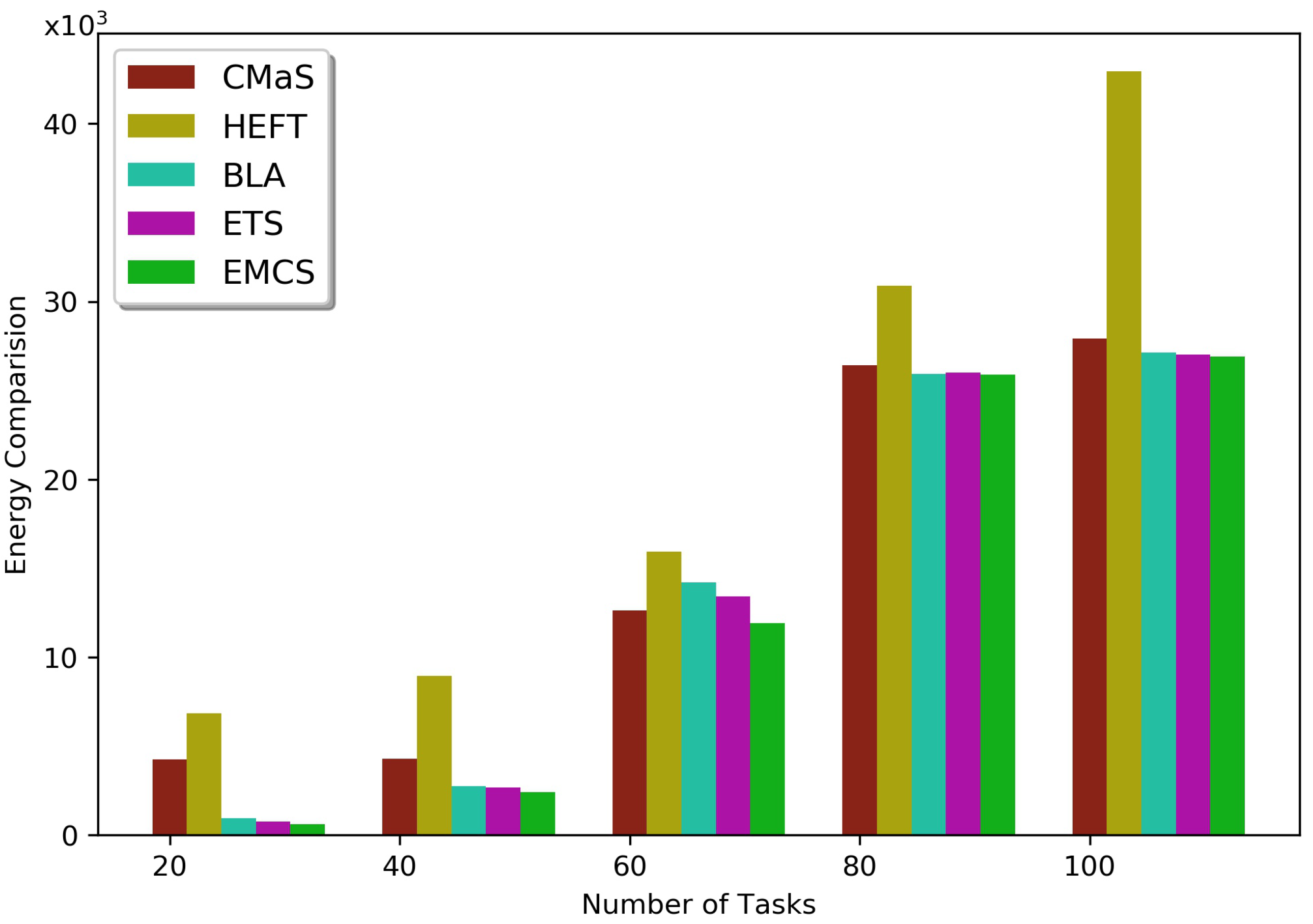
5.2. Results and Discussion

Several experiments were conducted with different scenarios. When 20 fog nodes and 5 cloud nodes were considered with tasks varied from 20 to 100, Figure 8 shows the computation of makespan for different numbers of tasks. The EMCS model performed 67.1% better than CMaS, 58.79% better than HEFT, 54.68% better than BLA and 47.81% better than ETS.

Regarding the cost of usage of cloud and fog (shown in Figure 9), it has been observed that HEFT has the highest cost, while EMCS has the lowest cost and CMaS, BLA and ETS have the average. HEFT focuses on the processing time of the task without considering other costs and energy. So, it has the highest cost. While compared with CMaS, EMCS can save 62.4% of the average cost; EMCS can save 26.41% of the average cost of BLA and 6.5% of average cost of ETS.

It is observed that the energy consumption is higher with an increase of task numbers in Figure 10. It is also observed that HEFT has the highest energy consumption compared to the others. EMCS saves 11.55% of the average energy of CMaS, 4.75% of the average energy of BLA and 3.19% of the average energy of ETS.

Next, the impact of cloud nodes in different algorithms (EMCS, CMaS, HEFT, BLA and ETS) with an increase in the nodes from 5 to 25 is evaluated. In this experiment, the number of processing nodes is fixed at 50 with varying cloud nodes from 5 to 25 generating different simulation results. Each cloud node has different parameter values. The results are shown in Figure 11, Figure 12 and Figure 13 which indicate that the makespan is decreased with the increase of cloud nodes in the network. As the cloud demands more processing cost and communication cost, the monetary cost is increased with the increasing of cloud nodes, and similarly, energy consumption is also increased with the increasing of cloud nodes. It is found that with the increase of clouds, the makespan of our algorithm EMCS is 64.21% better than that of CMaS, 30.41% better than HEFT, 11.62% better than BLA, and 7% better than ETS. It is observed in Figure 11 that there is an increase of makespan from 20 to 25 clouds in our proposed model, while the makespan in other algorithms is decreased.

In the case of cost comparison on increasing clouds from 5 to 25, the cost is increased in all the algorithms, while our model EMCS saves more cost than CMaS, HEFT, BLA, and ETS. It is observed in Figure 12 that our model is slightly better than BLA and ETS with increasing clouds from 5 to 15, and it is also better in the change of clouds from 15 to 25. Overall, the EMCS algorithm can save 21.81% of the average cost compared with BLA and 7.25% of the average cost compared with ETS.

Similarly, energy consumption is also increased with increasing the clouds from 5 to 25 in all the algorithms. Our model saves more energy than CMaS, HEFT, BLA and ETS. It is noticeable in Figure 13 that our model can save 8.24% of the average compared with BLA and 3.78% of the average compared with ETS, but the energy consumption of our model is almost the same with BLA and ETS when the number of clouds is set to 15.

Similarly, when the fog nodes are changed from 5 to 25 with a fixed number of processors at 50, the impact on makespan, cost, and energy consumption is shown in Figure 14, Figure 15 and Figure 16. The makespan is reduced with an increase in fog nodes which is noticeable in Figure 14. It is also found that our model is 6.94% better than BLA and 3.43% better than ETS.

The cost is varied when the fog nodes are changed from 5 to 25, as shown in Figure 15. It is noticeable that the cost is increased when the fog nodes are 15 and the cost of our model is almost the same as the cost of BLA and ETS at 20 fog nodes. The average cost of our model is 14.09% less than the average cost of BLA and 7.64% less than the average cost of ETS.

Similarly, following Figure 16, it is found that the energy is reduced with the increase of fog nodes from 5 to 20, but it is increased when there are 25 fog nodes. In addition, the energy consumption is similar at fog node 20 for our model, BLA and ETS. When the average energy consumption is considered, then our model consumes 31.75% less energy than BLA and 15.97% less energy than ETS.

So, it is observed from all the above results that a balance between cloud and fog nodes is required to give a better performance in terms of makespan, cost, and energy consumption. In addition, as the EMCS algorithm gives optimum makespan, cost and energy consumption, it is helpful for reducing global warming.

6. Conclusions

In this work, we adopt the combined cloud-fog architecture to schedule the set of dependent tasks. The evolutionary strategy-based EMCS algorithm is proposed, and its performance is evaluated with other methods such as CMaS [1], HEFT [13], BLA [14] and ETS [15]. By observing all the results, it is found that EMCS is better than CMaS by 67.1%, HEFT by 58.79%, BLA by 54.68% and ETS by 47.81% in terms of the average makespan with high performance on cost and energy consumption. EMCS is better than CMaS by 62.4%, BLA by 26.41% and ETS by 6.5% on average cost, and EMCS has reduced energy consumption compared with CMaS by 11.55%, BLA by 4.75% and ETS by 3.19%. The increase of cloud and fog nodes has a heavy impact on the network. Overall, our model is better than other algorithms with the change of cloud nodes from 5 to 25. It is observed that the makespan of EMCS is 11.62% better than the makespan of BLA and 7% better than the makespan of ETS. Similarly, the cost of EMCS is also reduced to 21.81% of the cost of BLA and 7.25% of the cost of ETS, and the energy consumption of EMCS is 8.24% less than BLA and 3.78% less than ETS. However, the makespan, cost, and energy consumption are almost the same in EMCS, BLA and ETS when the cloud node is set to 15. Similarly, with varying fog nodes from 5 to 25, comparing EMCS, BLA and ETS, the average estimation of EMCS is 6.94% better than BLA and 3.43% better than ETS in the case of makespan. Meanwhile, the average cost of EMCS is 14.09% less than BLA and 7.64% less than ETS, and the average energy consumption of EMCS is 32.75% less than BLA and 15.97% less than ETS. While considering the fog nodes at 20, the cost and energy consumption are almost the same in both EMCS, BLA and ETS.

So, from the overall result of the algorithm, it can be concluded that this algorithm will be a better solution for industry to use as it shows less energy, cost, and makespan that can reduce the carbon emmisions and decrease the global warming. In the future, we will try to implement more meta-heuristic algorithms to solve the scheduling problems. We will also expand our research by focusing on the priority, deadline constraint of the task and use of virtual machines in task scheduling.

References

1. Pham, X.Q.; Man, N.D.; Tri, N.D.T.; Thai, N.Q.; Huh, E.N. A cost-and performance-effective approach for task scheduling based on collaboration between cloud and fog computing. Int. J. Distrib. Sens. Netw. 2017, 13, 1550147717742073. [Google Scholar] [CrossRef] [Green Version]
2. Sahoo, K.S.; Tiwary, M.; Luhach, A.K.; Nayyar, A.; Choo, K.K.R.; Bilal, M. Demand–Supply-Based Economic Model for Resource Provisioning in Industrial IoT Traffic. IEEE Internet Things J. 2021, 9, 10529–10538. [Google Scholar] [CrossRef]
3. Nguyen, B.M.; Thi Thanh Binh, H.; Do Son, B. Evolutionary algorithms to optimize task scheduling problem for the IoT based bag-of-tasks application in cloud–fog computing environment. Appl. Sci. 2019, 9, 1730. [Google Scholar] [CrossRef] [Green Version]
4. Fog Computing and the Internet of Things: Extend the Cloud to Where the Things Are. Available online: https://studylib.net/doc/14477232/fog-computing-and-the-internet-of-things–extend (accessed on 2 September 2021).
5. Naha, R.K.; Garg, S.; Georgakopoulos, D.; Jayaraman, P.P.; Gao, L.; Xiang, Y.; Ranjan, R. Fog computing: Survey of trends, architectures, requirements, and research directions. IEEE Access 2018, 6, 47980–48009. [Google Scholar] [CrossRef]
6. Mukherjee, M.; Shu, L.; Wang, D. Survey of fog computing: Fundamental, network applications, and research challenges. IEEE Commun. Surv. Tutor. 2018, 20, 1826–1857. [Google Scholar] [CrossRef]
7. Bhoi, S.K.; Panda, S.K.; Jena, K.K.; Sahoo, K.S.; Jhanjhi, N.; Masud, M.; Aljahdali, S. IoT-EMS: An Internet of Things Based Environment Monitoring System in Volunteer Computing Environment. Intell. Autom. Soft Comput. 2022, 32, 1493–1507. [Google Scholar] [CrossRef]
8. Mao, L.; Li, Y.; Peng, G.; Xu, X.; Lin, W. A multi-resource task scheduling algorithm for energy-performance trade-offs in green clouds. Sustain. Comput. Inform. Syst. 2018, 19, 233–241. [Google Scholar] [CrossRef]
9. Wu, C.; Li, W.; Wang, L.; Zomaya, A. Hybrid evolutionary scheduling for energy-efficient fog-enhanced internet of things. IEEE Trans. Cloud Comput. 2018, 9, 641–653. [Google Scholar] [CrossRef]
10. Kabirzadeh, S.; Rahbari, D.; Nickray, M. A hyper heuristic algorithm for scheduling of fog networks. In Proceedings of the 2017 21st Conference of Open Innovations Association (FRUCT), Helsinki, Finland, 6–10 November 2017; pp. 148–155. [Google Scholar]
11. Ma, X.; Gao, H.; Xu, H.; Bian, M. An IoT-based task scheduling optimization scheme considering the deadline and cost-aware scientific workflow for cloud computing. Eurasip J. Wirel. Commun. Netw. 2019, 2019, 249. [Google Scholar] [CrossRef] [Green Version]
12. Hoang, D.; Dang, T.D. FBRC: Optimization of task scheduling in fog-based region and cloud. In Proceedings of the 2017 IEEE Trustcom/BigDataSE/ICESS, Sydney, Australia, 1–4 August 2017; pp. 1109–1114. [Google Scholar]
13. Topcuoglu, H.; Hariri, S.; Wu, M.Y. Performance-effective and low-complexity task scheduling for heterogeneous computing. IEEE Trans. Parallel Distrib. Syst. 2002, 13, 260–274. [Google Scholar] [CrossRef]
14. Bitam, S.; Zeadally, S.; Mellouk, A. Fog computing job scheduling optimization based on bees swarm. Enterp. Inf. Syst. 2018, 12, 373–397. [Google Scholar] [CrossRef]
15. Abdulredha, M.N.; Bara’a, A.A.; Jabir, A.J. An Evolutionary Algorithm for Task scheduling Problem in the Cloud-Fog environment. In Proceedings of the Journal of Physics: Conference Series; IOP Publishing: Bristol, UK, 2021; Volume 1963, p. 012044. [Google Scholar]
16. Liu, Q.; Wei, Y.; Leng, S.; Chen, Y. Task scheduling in fog enabled internet of things for smart cities. In Proceedings of the 2017 IEEE 17th International Conference on Communication Technology (ICCT), Chengdu, China, 15 May 2017; pp. 975–980. [Google Scholar]
17. Liu, L.; Qi, D.; Zhou, N.; Wu, Y. A task scheduling algorithm based on classification mining in fog computing environment. Wirel. Commun. Mob. Comput. 2018, 2018, 2102348. [Google Scholar] [CrossRef] [Green Version]
18. Xu, J.; Hao, Z.; Zhang, R.; Sun, X. A method based on the combination of laxity and ant colony system for cloud-fog task scheduling. IEEE Access 2019, 7, 116218–116226. [Google Scholar] [CrossRef]
19. Benblidia, M.A.; Brik, B.; Merghem-Boulahia, L.; Esseghir, M. Ranking fog nodes for tasks scheduling in fog-cloud environments: A fuzzy logic approach. In Proceedings of the 2019 15th International Wireless Communications & Mobile Computing Conference (IWCMC), Tangier, Morocco, 24–28 June 2019; pp. 1451–1457. [Google Scholar]
20. Zhao, H.; Qi, G.; Wang, Q.; Wang, J.; Yang, P.; Qiao, L. Energy-efficient task scheduling for heterogeneous cloud computing systems. In Proceedings of the 2019 IEEE 21st International Conference on High Performance Computing and Communications, IEEE 17th International Conference on Smart City, IEEE 5th International Conference on Data Science and Systems (HPCC/SmartCity/DSS), Zhangjiajie, China, 10–12 August 2019; pp. 952–959. [Google Scholar]
21. Boveiri, H.R.; Khayami, R.; Elhoseny, M.; Gunasekaran, M. An efficient Swarm-Intelligence approach for task scheduling in cloud-based internet of things applications. J. Ambient. Intell. Humaniz. Comput. 2019, 10, 3469–3479. [Google Scholar] [CrossRef]
22. Aladwani, T. Scheduling IoT healthcare tasks in fog computing based on their importance. Procedia Comput. Sci. 2019, 163, 560–569. [Google Scholar] [CrossRef]
23. Jena, R. Energy efficient task scheduling in cloud environment. Energy Procedia 2017, 141, 222–227. [Google Scholar] [CrossRef]
24. Ben Alla, S.; Ben Alla, H.; Touhafi, A.; Ezzati, A. An efficient energy-aware tasks scheduling with deadline-constrained in cloud computing. Computers 2019, 8, 46. [Google Scholar] [CrossRef] [Green Version]
25. Wang, J.; Li, D. Task scheduling based on a hybrid heuristic algorithm for smart production line with fog computing. Sensors 2019, 19, 1023. [Google Scholar] [CrossRef] [Green Version]
26. Rahbari, D.; Nickray, M. Scheduling of fog networks with optimized knapsack by symbiotic organisms search. In Proceedings of the 2017 21st Conference of Open Innovations Association (FRUCT), Helsinki, Finland, 6–10 November 2017; pp. 278–283. [Google Scholar]
27. Rahbari, D.; Nickray, M. Low-latency and energy-efficient scheduling in fog-based IoT applications. Turk. J. Electr. Eng. Comput. Sci. 2019, 27, 1406–1427. [Google Scholar] [CrossRef] [Green Version]
28. Wu, H.Y.; Lee, C.R. Energy efficient scheduling for heterogeneous fog computing architectures. In Proceedings of the 2018 IEEE 42nd annual computer software and applications conference (COMPSAC), Tokyo, Japan, 23–27 July 2018; Volume 1, pp. 555–560. [Google Scholar]
29. Tang, C.; Hao, M.; Wei, X.; Chen, W. Energy-aware task scheduling in mobile cloud computing. Distrib. Parallel Databases 2018, 36, 529–553. [Google Scholar] [CrossRef]
30. Li, G.; Yan, J.; Chen, L.; Wu, J.; Lin, Q.; Zhang, Y. Energy consumption optimization with a delay threshold in cloud-fog cooperation computing. IEEE Access 2019, 7, 159688–159697. [Google Scholar] [CrossRef]
31. Mazumdar, N.; Nag, A.; Singh, J.P. Trust-based load-offloading protocol to reduce service delays in fog-computing-empowered IoT. Comput. Electr. Eng. 2021, 93, 107223. [Google Scholar] [CrossRef]
32. Singh, H.; Tyagi, S.; Kumar, P. Cloud resource mapping through crow search inspired metaheuristic load balancing technique. Comput. Electr. Eng. 2021, 93, 107221. [Google Scholar] [CrossRef]
33. Lin, K.; Pankaj, S.; Wang, D. Task offloading and resource allocation for edge-of-things computing on smart healthcare systems. Comput. Electr. Eng. 2018, 72, 348–360. [Google Scholar] [CrossRef]
34. Ibrahim, H.; Aburukba, R.O.; El-Fakih, K. An integer linear programming model and adaptive genetic algorithm approach to minimize energy consumption of cloud computing data centers. Comput. Electr. Eng. 2018, 67, 551–565. [Google Scholar] [CrossRef]
35. Shishido, H.Y.; Estrella, J.C.; Toledo, C.F.M.; Arantes, M.S. Genetic-based algorithms applied to a workflow scheduling algorithm with security and deadline constraints in clouds. Comput. Electr. Eng. 2018, 69, 378–394. [Google Scholar] [CrossRef]
36. Kumar, M.; Sharma, S.C. Deadline constrained based dynamic load balancing algorithm with elasticity in cloud environment. Comput. Electr. Eng. 2018, 69, 395–411. [Google Scholar] [CrossRef]
37. Panda, S.K.; Nanda, S.S.; Bhoi, S.K. A pair-based task scheduling algorithm for cloud computing environment. J. King Saud-Univ.-Comput. Inf. Sci. 2022, 34, 1434–1445. [Google Scholar] [CrossRef]
38. Bhoi, S.; Panda, S.; Ray, S.; Sethy, R.; Sahoo, V.; Sahu, B.; Nayak, S.; Panigrahi, S.; Moharana, R.; Khilar, P. TSP-HVC: A novel task scheduling policy for heterogeneous vehicular cloud environment. Int. J. Inf. Technol. 2019, 11, 853–858. [Google Scholar] [CrossRef]
39. Panda, S.K.; Bhoi, S.K.; Khilar, P.M. A Semi-Interquartile Min-Min Max-Min (SIM 2) Approach for Grid Task Scheduling. In Proceedings of the International Conference on Advances in Computing, Kumool, India, 22–23 April 2013; pp. 415–421. [Google Scholar]
40. Abd Elaziz, M.; Abualigah, L.; Attiya, I. Advanced optimization technique for scheduling IoT tasks in cloud-fog computing environments. Future Gener. Comput. Syst. 2021, 124, 142–154. [Google Scholar] [CrossRef]
41. Guevara, J.C.; da Fonseca, N.L. Task scheduling in cloud-fog computing systems. Peer-Peer Netw. Appl. 2021, 14, 962–977. [Google Scholar] [CrossRef]
42. Ali, H.S.; Rout, R.R.; Parimi, P.; Das, S.K. Real-Time Task Scheduling in Fog-Cloud Computing Framework for IoT Applications: A Fuzzy Logic based Approach. In Proceedings of the 2021 International Conference on COMmunication Systems & NETworkS (COMSNETS), Bangalore, India, 5–9 January 2021; pp. 556–564. [Google Scholar]
43. Movahedi, Z.; Defude, B. An efficient population-based multi-objective task scheduling approach in fog computing systems. J. Cloud Comput. 2021, 10, 1–31. [Google Scholar] [CrossRef]
44. Wang, S.; Zhao, T.; Pang, S. Task scheduling algorithm based on improved firework algorithm in fog computing. IEEE Access 2020, 8, 32385–32394. [Google Scholar] [CrossRef]
45. Bian, S.; Huang, X.; Shao, Z. Online task scheduling for fog computing with multi-resource fairness. In Proceedings of the 2019 IEEE 90th Vehicular Technology Conference (VTC2019-Fall), Honolulu, HI, USA, 22–25 September 2019; pp. 1–5. [Google Scholar]
46. Karagiannis, V. Compute node communication in the fog: Survey and research challenges. In Proceedings of the IoT-Fog 2019—2019 Workshop on Fog Computing and the IoT, Montreal, QC, Canada, 15–18 April 2019; pp. 36–40. [Google Scholar]
47. BIN PACKING Proof of NP Completeness and Hardness. Available online: https://cs.ubishops.ca/home/cs567/more-np-complete/rangasamy-bin-packing.pdf (accessed on 2 September 2021).
48. Azizi, S.; Shojafar, M.; Abawajy, J.; Buyya, R. Deadline-aware and energy-efficient IoT task scheduling in fog computing systems: A semi-greedy approach. J. Netw. Comput. Appl. 2022, 201, 103333. [Google Scholar] [CrossRef]
Figure 1. System architecture.
Sustainability 14 15096 g001
Figure 2. The process flow model on C l o u d _ f o g system.
Sustainability 14 15096 g002
Figure 3. Task and Processor Graph.
Sustainability 14 15096 g003
Figure 4. Chromosome encoding.
Sustainability 14 15096 g004
Figure 5. Two-point crossover operation.
Sustainability 14 15096 g005
Figure 6. Mutation operation.
Sustainability 14 15096 g006
Figure 7. Flowchart for EMCS.
Sustainability 14 15096 g007
Figure 8. Comparing makespan of EMCS with other methods.
Sustainability 14 15096 g008
Figure 9. Cost comparison of EMCS with other methods.
Sustainability 14 15096 g009
Figure 10. Energy comparison of EMCS with other methods.
Sustainability 14 15096 g010
Figure 11. Impact of cloud nodes on makespan.
Sustainability 14 15096 g011
Figure 12. Impact of cloud nodes on cost.
Sustainability 14 15096 g012
Figure 13. Impact of cloud nodes on energy consumption.
Sustainability 14 15096 g013
Figure 14. Impact of fog nodes on makespan.
Sustainability 14 15096 g014
Figure 15. Impact of fog nodes on cost.
Sustainability 14 15096 g015
Figure 16. Impact of fog nodes on energy consumption.
Sustainability 14 15096 g016