Article

Estimation of Indoor Temperature Increments in Summers Using Heat-Flow Sensors to Assess the Impact of Roof Slab Insulation Methods

1
Department of Architecture, Graduate School of Advanced Science and Engineering, Hiroshima University, Hiroshima 739-8527, Japan
2
Technical Service Team, Research & Development Group, Dyflex Co., Ltd., Chiba 273-0027, Japan
*
Author to whom correspondence should be addressed.
Sustainability 2022, 14(22), 15127; https://doi.org/10.3390/su142215127
Submission received: 17 October 2022 / Revised: 10 November 2022 / Accepted: 11 November 2022 / Published: 15 November 2022
(This article belongs to the Special Issue Sustainability and Indoor Environmental Quality)

Abstract

:
Improving the thermal insulation performance of buildings is crucial for saving energy. Currently, the insulation performance can be quantified based on the thermal resistance and thermal transmittance (U-value). However, for owners, these data are not readily available for the verification of different insulation methods. To address this, a solution could involve establishing a connection between specialized evaluation indicators and temperature, a common physical quantity. In this study, static and dynamic heat-transfer experiments were performed using an environmental simulation chamber and heat-flow sensors. Based on the tests, a simple predictive formula for the heat-flow density over time was established. After analyzing a full-scale building model, six cases of the heat-flow density versus temperature rise in indoor environments were obtained. This approach may aid owners in visually assessing the insulation performance of buildings by establishing a conversion relationship between the heat-flow density and temperature. In addition, the performance of 14 experimental specimens, including self-developed and code-documented thermal insulation materials and construction methods, was evaluated. In the simulations, after turning off indoor cooling equipment for 6 h during hot summers, the average indoor temperature increase for a roof with insulation was only 52% of that without insulation.

1. Introduction

Currently, energy conservation and emission reduction are becoming increasingly important. Accordingly, to achieve these objectives, the building sector has strict requirements. In 2020, the building sector accounted for 36% of the global energy demand and 37% of energy-related CO2 emissions [1]. In particular, owing to its high energy consumption and predominant use of refrigerants with significant global warming potential, space cooling is one of the major contributors to climate change [1]. According to the International Energy Agency, the energy utilization for space cooling has doubled since 2000. The Programme for Energy Efficiency in Buildings reports that the energy needs of space cooling could triple by 2050, particularly in hot and tropical countries. To address this issue, improving the thermal insulation efficiency of buildings and raising public awareness seem to be effective approaches [1].
Ensuring the good insulation performance of building envelopes is important for improving their energy efficiency and reducing structural deterioration factors [2,3,4,5]. During summers, 50% to 70% of the total energy may penetrate building structures from roof elements [6,7,8], as they are highly exposed to solar radiation for extended periods. Therefore, the use of insulation solutions on roof elements can limit the entry of heat into a building’s interior space, thereby reducing the thermal load and, consequently, the demand for refrigeration equipment to provide comfort to occupants. From this perspective, at the structural level, possible solutions to address this issue include the use of green roofs [9,10,11,12], reflective systems [13,14,15], and radiant barrier configurations [16,17,18,19]. Alternatively, at the material level, various thermal insulation materials have been widely developed because they are less restricted by building types. Notably, good insulation materials can maintain thermal comfort inside a housing environment and prevent heat exchange with the surrounding environment.
Currently, indicators for evaluating the performance of insulation materials include the thermal conductivity and thermal resistance, and the common measurement methods include the heat-flow method [20] and the guarded heat plate method (GHP) [21]. However, a typical building envelope may consist of multiple layers such as the substrate, insulation, and decorative layers, which makes it difficult to determine the physical properties of each layer of the element. Therefore, in actual practice, the indicators for evaluating the thermal insulation performance of building elements generally include the total thermal resistance and thermal transmittance (U-value) [22]. Additionally, the common measurement methods for the U-value include the calibrated and guarded hot box method (CHB) [23], heat-flow meter method [24], infrared thermography method [25], and temperature-based method [26,27]. However, most of these measurements must satisfy the approximate steady-state heat-transfer conditions for large temperature differences. Therefore, in situ measurements over at least 72 h in specific seasons are usually required to obtain reliable data [22,28]. Alternatively, it is necessary to filter the data [29] or use dynamic theory to consider the fluctuations, hysteresis, and decay of the heat-flow density and temperature [30,31,32].
So far, based on these indicators, the effectiveness of various insulation materials has been evaluated in several studies. Su et al. designed and fabricated basalt fiber-reinforced plastic roof panels with core materials of extruded polystyrene, polyurethane, and rock wool. They conducted a series of investigations on the thermal conductivity, U-values, and thermal bridge effects of these experimental specimens by means of GHP and CHB experiments and Abaqus software analysis [33]. Geoola et al. designed a guarded hot box wherein the use of a thermal screen could reduce the U-value by approximately 30% at different wind speeds and temperature differences [34]. Pasupathy et al. performed experimental investigations and numerical simulations on the thermal behavior of a residential roof using phase-change materials (PCMs) [35]. In a transient analysis, Prakash et al. demonstrated that the use of PCMs can reduce the heat entering a room by 13% [36]. Costantine et al. conducted experimental and numerical investigations on the temperature, humidity, and heat flux in an office with hemp-lime insulation [37]. The ability of natural mesoporous materials to reduce surface temperatures was validated based on both steady-state and periodic experiments by Rahman et al. [38]. Altin et al. built three full-scale buildings and conducted temperature, moisture, and sound tests on boron-doped sheep wool, expanded polystyrene, and rock wool insulation [39]. Yin et al. carried out in situ tests on the thermal performance of a double-layered dome with aerogel-glass wool insulation and provided numerical analysis data for the design of the combination of insulation materials [40]. Hasan et al. investigated roof insulation in Iraq and discovered that certain combinations of insulation could reduce the heat flow by more than 79% [41]. Kuma et al. measured the thermal conductivity of insulation materials available in the Indian market using an automatic guarded hot plate apparatus and computed the thermal resistance and thermal transmittance of 112 wall and roof sectors [42]. Zhao et al. evaluated the bulk density, thermal conductivity, water absorption, and compressive strength of a large number of environment-friendly building insulation materials. They also selected seven of the most competitive insulation materials using the city of Harbin, China, as an example, by life-cycle cost [43].
To better address the energy management problems encountered by building owners, the economic aspects and applications of common building insulation materials, in addition to their performance characteristics, were also discussed by Al-Hamoud and Aditya et al. [44,45]. Halwatura et al. investigated the impact of insulated roof slabs on air-conditioning loads and estimated their life-cycle cost benefits [46]. Papadopoulos discussed various aspects of insulation materials, including their environmental and public health impacts, within the framework of legislation and the market [47]. Notably, in most cases, the evaluation indicators are targeted toward practitioners in the building industry. However, for owners, it is sometimes difficult to intuitively predict the insulation performance. We believe that establishing a connection between professional evaluation indicators and temperature, a common physical quantity, may be a solution to this issue.
The purpose of this study was to establish a relationship between heat-flow values and temperature for evaluating the thermal insulation performance of building elements. To that end, static and dynamic heat-transfer experiments were conducted on two factory roof slab specimens using an environmental simulation chamber and heat-flow sensors. A relationship between heat-flow density and time has been established, and it can evaluate the insulation performance in the field in the case of using heat-flow sensors. Six simulation cases were analyzed by determining the relationship between the heat-flow density and temperature increase in an indoor space using a simple full-scale building model. In addition, the insulation performance of 14 experimental specimens was evaluated under steady-state heat-transfer conditions, including self-developed and commercially available insulation materials and construction methods for factory roof slabs.

2. Materials and Methods

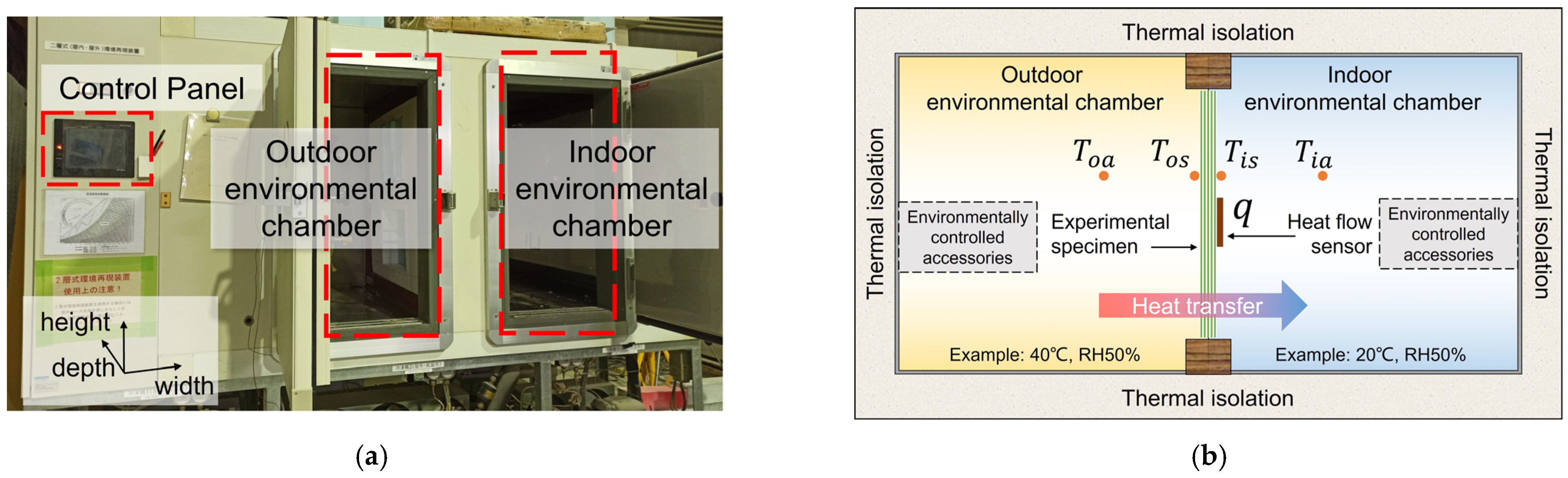
2.1. Environmental Simulation Chamber

The experiment involved in this study used an environmental simulation apparatus with independently controlled dual chambers, as shown in Figure 1a. The apparatus had effective insulation properties and a sensitive control system. Both chambers had the same dimensions: a width of 955 mm, height of 1100 mm, and depth of 1100 mm. The chambers were equipped with semi-enclosed environmentally controlled accessories, including sensors, blowers, and chillers. Aluminum alloy sheets formed the inner walls of the chambers. The temperature of the outdoor chamber could be controlled in the range of −20 to 40 °C, and its relative humidity could be controlled from 40% to 90%. The outdoor chamber was also equipped with an infrared lamp-based radiant heating function and a simulated precipitation function. The controllable temperature range of the indoor chamber was 4 °C to 40 °C, and the relative humidity ranged from 40% to 90%. The experimental setup is illustrated in Figure 1b.

2.2. Heat-Flow Sensors

Details pertaining to the heat-flow sensors used in the experiments are listed in Table 1. The surface temperatures and heat-flow densities were measured by connecting a heat-flow sensor to the surface of the specimens. A specialized thermally conductive double-sided adhesive tape was used to attach the sensors while preventing the adherence of foreign objects or the formation of air layers. In addition to the increase or decrease in temperatures, the heat-flow sensors also measured the direction of heat transfer. As depicted in Figure 2, the measured value was positive when the heat-flow sensor was placed on the low-temperature side and negative when it was placed on the high-temperature side. The smaller the absolute value of the heat-flow density, the better the insulation performance of the test specimen.

3. Heat-Transfer Performance Experiment

3.1. Experimental Specimen

The specimens used in the experiment had a width of 765 mm and height of 800 mm. The specimens were prepared using 0.8 mm-thick metal slabs as the substrates to simulate factory roofs, as illustrated in Figure 3. To mount the specimen slabs in the environmental simulation chamber, they were fitted using 30 mm × 45 mm foam frame strips. Therefore, in the experiment, the actual working area of the specimen had a width of 710 mm and height of 675 mm. Only a silicone acrylic coating was applied to specimen A1, as indicated in Table 2, whereas specimen A2 was subjected to a waterproof coating and a heat insulation layer.

3.2. Heat-Transfer Procedure and Setup

The heat-transfer process is shown in Figure 4. In Figure 4a, heat-transfer Pattern 1 simulates static heat transfer. At the beginning, the temperatures of both the outdoor and indoor chambers were set to 20 °C. The temperature of the indoor chamber was then held constant, and the outdoor chamber temperature was raised to 40 °C within the shortest possible duration. Over the next 10 h, a temperature difference of 20 °C was maintained between the two chambers. This temperature difference was large enough to reliably estimate the heat-transfer performance of the components. In Figure 4b, heat-transfer Pattern 2 simulated a dynamic heat transfer. The temperatures of the outdoor chamber and the indoor chamber were set to 40 °C and 20 °C, respectively. After reaching the balanced state, the power to the indoor chamber was individually turned off. This can simulate the situation of turning off the indoor air conditioner in real summer life. The temperature change in the indoor chamber was recorded while the outdoor temperature was maintained at 40 °C. A small air-circulation fan was used to minimize the air temperature differential in the indoor chamber after the power was turned off. However, as high-velocity winds can affect the results of heat-flow sensors, air was circulated in the chamber at a speed of less than 0.5 m/s. Further, data analysis was performed depending on the time at which the power was turned off. This was used as the initial time (t = 0). In addition, because the effect of humidity was not the focus of our discussion, the relative humidity of the chamber was set to 50% in all the experiments.
During the experiments, data were recorded at 30 s intervals. In the preparation phase of the experiment, the positions of 10 heat-flow density and 29 temperature measurement points were calibrated (Figure 5). The results indicated that measurement points located at the geometric center could represent the average values of the corresponding space. Therefore, the measurement points for the heat-flow density and temperature in this experiment were set according to the configuration of black circles depicted in Figure 5.

3.3. Results and Discussions

For heat-transfer Pattern 1, the results of the temperature and heat flow-density are shown in Figure 6 and Figure 7, respectively. The thermal transmittance (U-value) was calculated using Equation (1):
U ( t ) = q ( t ) | T i a ( t ) T o a ( t ) |
The results are shown in Figure 8. In Equation (1), U(t) and q(t) indicate the U-value (W/(m2 °C)) and heat-flow density (W/m2) of the specimen, respectively. Toa and Tia denote air temperatures in the outdoor and indoor chambers, respectively. In heat-transfer Pattern 1, the middle 8 h, that is, 3–11 h of the experimental procedure, were considered to indicate a true steady state. The mean values and standard deviations (σ) of the experimental data for this period are listed in Table 3.
In Figure 6a, during the first 2 h, the air temperature in both chambers was 20 °C, and almost no temperature difference was noted. Following this, the outdoor chamber temperature was set to increase rapidly while the indoor chamber temperature was maintained constant. During the heat-transfer process, the temperatures of both the indoor and outdoor chambers fluctuated around approximately 40 ± 2.2 and 20 ± 0.7 °C, respectively, which roughly satisfied the preset environmental conditions. In addition, the air temperature difference (|TiaToa|) for specimen A1 was approximately 1.0 °C greater than that for specimen A2. This difference could be explained by the poor insulation properties of specimen A1, which was extremely thin. As shown in Figure 6b, specimen A1 produced only a small difference between the indoor and outdoor surface temperatures (|Tis − Tos|), which was approximately 0.4 °C. In contrast, specimen A2 produced both a higher outdoor surface temperature (Tos = 35.0 °C) and lower indoor surface temperature (Tis = 23.3 °C). This difference in temperature between the two surfaces (|TisTos|) of specimen A2 was significant at approximately 11.7 °C. This indicates that the application of an insulation material to a metal slab can effectively increase the thermal resistance of the element to achieve thermal insulation.
Figure 7 illustrates the heat-flow density results for heat-transfer Pattern 1. The corresponding data were acquired using the heat-flow sensor placed at the central position, as indicated in Figure 5. During the first 2 h, no heat transfer was noted, and the heat-flow density fluctuated around zero. After the first 2 h, the heat-flow density of specimen A1 rapidly increased to approximately 113.4 W/m2. Conversely, the heat-flow density of specimen A2 increased at a slower rate and fluctuated at approximately 44.4 W/m2. Thus, the insulating material reduced the heat transfer by more than half.
In Figure 8, which depicts the thermal transmittance results, the U-values fluctuated considerably for the 2 h during which almost no temperature difference was noted between the indoor and outdoor environments. Because heat transfer was almost absent during such periods, the data could not be used to calculate the U-values. During the middle 8 h of static heat transfer, specimen A1 exhibited a larger U-value of approximately 6.0 W/(m2∙°C). Under the same conditions, the U-value of specimen A2 was significantly reduced at approximately 2.2 W/(m2∙°C), and the thermal insulation performance of the element improved.
In heat-transfer Pattern 2, the time point (t = 0) at which the power to the indoor chamber was turned off, depicted in Figure 4b, was used as the starting point for data collection. The indoor surface heat-flow density and indoor chamber temperature results for the specimen are presented in Figure 9. Notably, because the wiring of the heat-flow sensor at the central position (Figure 5) had some flaws, the average values measured by the other two heat-flow sensors are presented here. Initially, the temperature difference between the indoor and outdoor chambers was the highest; thus, the heat transfer was the most intense. As the temperature difference decreased over time, heat transfer slowed. For specimen A1, the heat-flow density decreased rapidly from >100 W/m2 to zero. After approximately 13 h, the chamber air temperature almost stopped increasing, implying the end of dynamic heat transfer. For specimen A2, the heat-transfer reduction process was slightly slower. The initial heat-flow density was about 50 W/m2, which required about 24 h to gradually approach zero. A similar conclusion can be drawn from the temperature results, wherein, after 24 h, the dynamic heat-transfer process was almost complete. It is worth noting that, during the first 10 min, a rapid decrease in heat-flow density occurred. This could be attributed to the heating mechanism of the environmental simulation chamber. Note that the outdoor chamber temperature was not maintained constant at 40 °C but rather fluctuated in small ranges, and heating to target temperature was only reinitiated when the lower temperature limit of the system was reached. The decrease in heat-flow density was the combined result of a decrease in the outdoor chamber temperature and a reduction in heat transfer.
The relationship between the heat-flow density and air temperature difference at each moment for heat-transfer Pattern 2 is shown in Figure 10. A linear relationship with a coefficient of determination of 0.92 or more was obtained for both specimens. According to the implications of physical quantities of the data, the slope of the approximation curve denotes the U-value of the specimen. Comparing these results with those of heat-transfer Pattern 1 (Table 3), it was observed that the U-values obtained for these two sets of experiments were almost the same. This indicates that the U-value of the specimen can also be obtained from this dynamic heat-transfer experiment.

4. Proposal for Simulating Building Thermal Insulation Performance

During the warmest seasons, improving the insulating performance of a roof can be highly effective in reducing the total energy penetrating a building. Notably, temperature is a better understood concept than heat. This is because temperature is a physical quantity that is commonly used by the public in their daily lives. However, the conversion of heat to temperature often requires specialized and complex models. This conversion is not conveniently achievable for owners with daily sensor usage. Therefore, in this section, we propose a relationship between the change in heat-flow density and time. This relationship can be used to help owners better establish a correlation between the heat-flow density and temperature when using heat-flow sensors by predicting the indoor temperature increase.

4.1. Simulation Formula for the Heat-Flux Density

Our proposal can be used to simulate a situation wherein the outdoor temperature is higher than the indoor temperature, as is often the case in summers. Notably, indoor temperature increases when cooling air conditioners in the building are turned off. The proposed method can roughly predict the heat-flow density in a building during this process. This corresponds exactly to the dynamic heat transfer described by Pattern 2 in Section 3.2. According to Figure 9, this proposal assumes that the variation law of heat-flow density with time conforms to an exponential function. To simplify this model, we use only two variables, q0 and α, as presented in Equation (2):
q S i m u . ( t ) = q 0 · e α t
In this equation, q0 denotes the average of several heat flow densities obtained during static heat transfer. The data in Table 3 are referenced in this calculation; thus, the q0 values for specimens A1 and A2 were 113.4 W/m2 and 44.4 W/m2, respectively. However, in case of field limitations, q0 can also refer to the heat-flow density at any point when the air conditioner is turned off (t = 0). It should be noted that the calculated temperature result will be greater when the employed q0 is larger than the actual average heat-flow density, and vice versa. The other symbol α is a dimensionless quantity that indicates the rate of heat-flow density change with time. The larger the absolute value of α, the faster the change in the heat-flow density. The α value is calculated inversely based on the time corresponding to the end of the heat-transfer process (tend). According to the respective physical meanings, at moment tend, q(t) should be minimal. Because the exponential function can only be infinitely close to, but not equal to, zero, the value of qsimu.(tend) is simplified to 1. Therefore, the formula for α is expressed by Equation (3):
α = ln ( 1 / | q 0 | ) / t e n d .
According to Figure 9, the approximate values of tend for specimens A1 and A2 were considered as 13 and 24, respectively, as the temperature change of the corresponding experimental specimen in that hour was only 0.1 °C.
Subsequently, the rise in temperature was calculated. For dynamic heat transfer, the outdoor chamber temperature was held at approximately 40 °C after the power was turned off in the indoor chamber. The quantity of heat (Q) continuously penetrating the indoor chamber through the specimen was calculated using Equation (4):
Q t o t ( t ) = 0 t q S i m u . ( t ) d t · A ,
where the area A had a heat inflow of approximately 0.048 m2 in this experiment. During the heat-transfer process, the air, aluminum alloy inner wall, and other accessories in the indoor chamber were heated at the same rate. The relationship between the quantity of heat (Q) absorbed and the temperature increase (∆T) is presented in Equations (5) and (6), respectively:
Q a ( t ) = m a · c a · Δ T ( t ) ,
Q A l ( t ) = m A l · c A l · Δ T ( t ) ,
where the air specifically refers to the air in the volume of the indoor chamber. The mass ma and specific heat capacity ca of air were 1.40 kg and 1007 J/(kg·°C), respectively. The corresponding quantities for the aluminum alloy inner wall and environmental controlling accessories were estimated using the measurable surface area and thickness of the aluminum alloy. Thus, the mAl and cAl values were 25 kg and 900 J/(kg·°C), respectively. In addition, heat loss primarily comprised the loss caused by the chamber wall and the flanking loss of the specimen slab, which was calculated according to Equation (7):
Q l ( t ) = ( 1 η ) · Q t o t ( t ) .
The smaller the specimen thickness, the greater the flanking loss, and the lower the heating efficiency [48,49]. The efficiency η values for specimens A1 and A2 were considered as constants with values of 85% and 95%, respectively. The heat-transfer process followed the law of conservation of energy with Equation (8):
Q t o t ( t ) = Q a ( t ) + Q A l ( t ) + Q l ( t ) ,
and the temperature variation curve for the indoor chamber air could be obtained using Equation (9):
T i a ( t ) = T i a ( t = 0 ) + Δ T ( t ) ,
where the initial value of the indoor chamber air temperature (Tia (t = 0)) was 20 °C.
The experimental data were plotted against the simulation results, as in Figure 11. To clearly present the data points, unlike in Figure 9, the time interval for the experimental data scatter was decreased to one per hour. As can be seen, the trend of heat-flow density decreasing with time is well-fitted in Figure 11. For specimen A1, the fluctuations in the experimental data after 8 h were caused by high-frequency changes in the outdoor chamber temperature. However, this was an experiment-specific deviation that did not need to be filtered. Moreover, for the quantity of heat, this fluctuation did not have a significant effect on the indoor temperature change. Notably, the quantity of heat refers to the area between the heat-flow density curve and horizontal time axis curve. The temperature-change curve was determined using the simulated heat-flow density curve. This curve also exhibited a trend similar to that of the experimental data. This implies that the heat-flow simulation formula can be used to roughly estimate the rise in the indoor space temperature.

4.2. Simple Full-Scale Building Model

Further, in our analysis, simplified heat-transfer simulations were performed on a full-scale factory building model using Equation (2). Note that the scope of the following discussion encompasses the heat-transfer process that occurs during summers. The initial state (t = 0) indicates the time at which the indoor air conditioner is turned off. Heat is continuously transferred from the outdoor environment to the indoor environment through roofs. The heat-transfer process is considered complete (t = tend) when the indoor air temperature reaches the same level as the outdoor temperature. The dimensions of the adopted building model are depicted in Figure 12.
Note that five cases are discussed in this section, and the corresponding details are listed in Table 4. In Cases 1 to 3, the roofs had the same thermal transmittance (1.0 W/m2·°C) and different initial indoor–outdoor temperature differences. The purpose was to discuss the effect of the initial indoor–outdoor temperature difference on the overall temperature rise. In Cases 3 to 5, the indoor–outdoor temperature difference was the same (15.0 °C), whereas the thermal transmittances of the roofs were varied. The purpose was to discuss the effect of the thermal transmittance of roofs on the indoor temperature rise.
The assumptions of the model calculations are presented below:
  • Only heat entering the building from the roof is considered;
  • In all cases, the effective quantity of heat (Qe) entering the building within 24 h heats the indoor air to a preset outdoor air temperature;
  • The effective quantity of heat (Qe) denotes the amount of heat used to heat the air, which is 30% of the total quantity of heat (Qtot). The remaining heat is assumed to be absorbed by factory machinery or lost via ventilation.
The variation in the heat-flow density with time was obtained using Equation (2). The q0 value in each case was calculated according to Equation (1) using the U-value and the indoor–outdoor temperature difference at t = 0. The α value was calculated inversely based on the end-time of the heat transfer (tend) using Equation (3). Here, tend was determined according to the second assumption and was obtained, as shown in the following Equation (10):
{     Q e ( t = 24 h ) = m a · c a · Δ T ( t = t e n d ) Q e ( t ) = η · Q t o t ( t ) Q t o t ( t ) = 0 t q S i m u . ( t ) d t · A Δ T ( t = t e n d ) = | T i a ( t = 0 ) T o a ( t = 0 ) |
where the mass ma and specific heat capacity ca of air in the factory were assumed to be 541.8 kg and 1007 J/(kg·°C), respectively. The value of η was considered as 30% according to the third assumption. Here, the working area A refers to a roof area of 90 m2.
The simulation results for the indoor temperature increase in 24 h (assumption 2) are illustrated in Figure 13. The data for the 6th h in the figure are labeled while considering the realistic duration of the high-temperature period during daytime. In Figure 13a, for the same insulation performance of the roof, the temperature difference between the indoor and outdoor environments plays a decisive role in the level of indoor temperature rise. For equivalent time periods, the higher the initial temperature difference, the higher the increase in temperature. Particularly in the first few hours, the temperature in Case 1 increased by 9.9 °C at 6 h. Figure 13b indicates that the insulation performance of the roof exerted a significant effect on the temperature change in the building. Moreover, in the first few hours, the temperature in Case 4, which involved a relatively poor insulation (U = 2.0 W/m2·°C), increased rapidly. Thus, heat from the outside was quickly transferred to the building. Conversely, the temperature in Case 5, which had better insulation (U = 0.5 W/m2·°C), increased at a much slower and more uniform rate. At the 6th h, the temperature rise in Case 5 (6.5 °C) was less than half of that in Case 4 (13.2 °C). This implies that a well-insulated roof can reduce indoor temperatures by decreasing the rate of heat influx into the building.

5. Evaluating the Thermal Insulation Performance of Various Roof Slabs

Improving the thermal insulation performance of a roof is important to provide a more comfortable indoor environment during warmer seasons. This is particularly true for buildings such as factories, which often possess large roof surface areas for equivalent building spaces. Therefore, balancing the heat entering through the roof results in considerable power consumption of cooling equipment. From this perspective, the better the insulation performance of roof slab elements, the greater the achievable energy savings. In this section, static heat-transfer experiments were conducted on specimens of commercially available insulation materials, self-developed insulation materials, and common construction methods. The thermal insulation performance of these roof slabs was evaluated using simple experiments and simulations.

5.1. Specimens and Experiment

The specimens involved in this section were square slabs with side lengths of 30 mm, as shown in Figure 14. The specimens were constructed using a fiber-reinforced concrete board as the substrate, and on top of this, waterproof or thermal insulation was applied. Details pertaining to each layer are listed in Table 5.
In Table 5, the listed sprayed polyurethane foam (SPF) specimen is a self-developed specimen sprayed with polyurethane foam insulation with a ten-fold expansion rate. The extruded polystyrene foam (XPS) is a molded thermal insulation material with a thermal conductivity of 0.028 W/m∙°C (JIS A 9521). The rigid polyurethane foam (PUF) is a molded thermal insulation material with a thermal conductivity of 0.023 W/m∙°C (JIS A 9521). All three types of insulation are highly durable, high-performance materials that resist moisture and prevent condensation. According to the type of material, SPF and PUF are both polyurethane insulations, while XPS is polystyrene insulation. The former has better insulation properties, while the latter is cheaper and less sensitive to moisture. According to the molding process, SPF is molded in situ by spraying and making it foam at the same time, while XPF and PUF are made into boards at the plant and cut into various sizes in situ as needed. The spraying process ensures the adhesion and fixation of the insulation to the substrate. It is not only limited to flat construction surfaces but also suitable for wave panels or metal-profiled cladding sheets. However, weather conditions such as natural winds for spraying operations should be regulated to take full account of their impact on the surrounding area. The molded thermal insulation is applicable to flat surfaces only and not suitable for small or cornered areas. The cutting and assembling part of the molded board tends to lose its insulation and airtightness [50], thus requiring additional treatment attention. However, the use of molded insulation requires less technology and has economic advantages.
Specimens B1 through B5 were SPF insulation systems that could be used to elucidate the effects of each layer on the insulation performance. Specimen B3 was coated with a rapid-spray polyurethane seal for waterproofing. Specimen B4 had a standard construction with a 10 mm-thick SPF insulation system. The 20 mm-thick specimen (B5) was used for special construction in individual regions.
Specimens C1 through E1 were based on various waterproofing and thermal insulation constructions specified in JASS 8 [51]. Among them, specimens C1 and C2 were typified by adhesive waterproofing and insulation methods that could be used for flat concrete roofs. The two-sided adhesive butyl system allows the insulation to be bonded to the substrate, eliminating the need for anchors and thus avoiding thermal bridging. Moreover, the butyl sheet is waterproof, making the system unaffected by the moisture of the substrate; thus, the insulation layer can be either polyurethane or polystyrene. Specimens D1 and D2 were asphalt waterproofing and rubber sheet waterproofing constructions, respectively. Asphalt waterproofing has been widely used since very early on, with excellent waterproofing performance and a high degree of reliability. However, it is difficult to remove it during the renovation, and in some cases the construction process is not environmentally friendly. The rubber sheet waterproof has good ductility and can follow the movement of the roof slab joints without breaking. In the case of renovation, it can be directly covered on the uppermost layer of the existing structure with simple construction and short construction period. However, the thickness of the rubber sheet waterproof is small; thus, it is sensitive to UV and impact, and in addition, the cost is high. Specimen E1 was a modified asphalt waterproofing construction used for mechanical fixation systems. This specimen refers to the waterproofing and insulation constructions of concrete flat roofs using metal anchors. Notably, the small specimen used butyl adhesive sheets instead of anchors to bond the layers. Mechanical fixation systems require less surface treatment of the substrate; however, since the insulation layer is in direct contact with the substrate, only insulation materials with low water absorption should be used.
All specimens were subjected to heat-transfer Pattern 1, as described in Section 3.2. The temperature difference between the indoor and outdoor air was 20 °C. The experimental setup is shown in Figure 15. A heat-flow sensor was set at the geometric center of the indoor surface of the specimen. The time interval for data recording was set to 5 min. The temperature of the environmental simulation chamber was set as indicated in Figure 4a.

5.2. Results and Discussions

The heat-flow density results for each specimen listed in Table 5 are presented in Figure 16. At the beginning of data recording, the heat flow was negative for some of the specimens. This was because the surface temperature of the specimens was below 20 °C at the beginning, owing to which heat flowed into the specimens from the indoor chamber. Within the first 2 h, the heat-flow density values for all specimens reached near zero. This indicates that no heat transfer occurred within the specimens and that both chambers had reached the preset temperature of 20 °C. After the 2nd h, the outdoor chamber temperature was set to rise rapidly (Figure 4a), resulting in a significant increase in the heat-flow density values of the specimens. Subsequently, the whole system gradually reached a steady state of heat transfer, with the heat-flow density fluctuating around a specific value. At the 12th h, the temperature difference between the two chambers disappeared, and the heat-flow density through the specimen then decreased rapidly. At the end of the experiment, there was no heat transfer; that is, the heat-flow density was zero. The calculation of the U-value requires experimental data of steady-state heat transfer at large temperature differences to evaluate the thermal insulation performance. The middle 8 h of the experiment were regarded to correspond to the true static heat transfer. Thus, the data from 3–11 h were averaged to evaluate the performance of the specimens.
In Figure 16a, the insulation properties of various insulation materials are clearly compared. Note that lower heat-flow density values indicate better thermal insulation performance. Among the specimens, the PUF specimen with a thickness of 30 mm demonstrated optimal thermal insulation performance. The average heat-flow density from the surface of the specimen to the indoor chamber was approximately 10.3 W/m2. In addition, the SPF insulation material exhibited an excellent insulation ability. The average heat-flow density of the SPF specimen with a thickness of 25 mm was approximately 17.8 W/m2.
As shown in Figure 16b, the specimens with more complete construction procedures demonstrated lower heat-flow densities and better thermal insulation performance. The average heat-flow density of the specimens without insulation layers (B1, B2, and B3) was about 60 W/m2, whereas that of specimens with insulation layers (B4 and B5) was about 20 W/m2. The difference between the two groups was evident, with a heat-transfer difference of approximately three times. The average heat-flow densities of specimens B1, B2, and B3 were 66.2 W/m2, 62.2 W/m2, and 61.7 W/m2, respectively. Therefore, it could be determined that the top coating and waterproofing layers also had certain insulation capacities. The data for specimen B2 fluctuated considerably, which can be explained since the experimental specimen was too thin and, therefore, particularly sensitive to temperature changes. The average heat-flow densities of specimens B4 and B5 were 23.8 W/m2 and 17.8 W/m2, respectively. The 10 mm-thick SPF insulation material demonstrated a good insulation effect, and the 20 mm-thick SPF insulation material further reduced the heat-flow density. However, in terms of efficiency per unit thickness, the 10 mm SPF may be more efficient. This implies that, for most building insulation constructions, selecting materials with excessive thicknesses is not essential; alternatively, striking a balance between the efficiency and economic benefits appears more reasonable.
Figure 16c indicates that the heat-flow densities of all the specimens were between 10 W/m2 and 15 W/m2, with minimal variation. The large fluctuations in the heat-flow density of specimen E1 could be explained by the effect of wind on the heat-flow sensor in the chamber during the experiment. This may also be attributed to the insufficient adhesion of the heat-flow sensor onto the surface of the specimen. The difference between different insulation materials for the same construction method can be determined by comparing specimens C1 and C2. The trend followed by the results for this group of experiments was the same as that depicted in Figure 16a; that is, the PUF insulation slightly outperformed the XPS insulation for the same thickness. By comparing specimens D1 and D2, the insulation effects of different waterproofing methods can be ascertained. Asphalt waterproofing may provide better insulation performance than rubber sheet waterproofing. The differences in the insulation fixation techniques can be obtained by comparing specimens C1 and E1. Evidently, the adhesion method results in better insulation than the mechanical fixation method. This could be related to the construction method itself, which increases the number of layers and the thickness of the specimen. It is worth noting that the adhesion method can also avoid thermal bridging resulting from the mechanical fixation method in actual constructions. In general, the difference in insulation performance between the specimens can be conveniently compared using a heat-flow sensor when the boundary conditions of heat transfer are the same.
The results of the average values of the heat-flow density and calculated heat transmittance (Equation (1)) for all specimens are summarized in Figure 17. The smaller the U-value, the better the thermal insulation of the specimens. The chamber temperature was the same in these experiments, which means that the boundary conditions of the specimens were the same. In this case, the trend of U-value and heat-flow density values should be the same for various specimens. In addition, insulating materials perform the insulation function by increasing the temperature gradient inside themselves. This means that excellent thermal insulations reduce the heat exchange between the entire specimen and the chamber environment. Thus, the specimens with better thermal insulation may have smaller heat-flow density values. However, the heat-flow density of specimen E1 was greater than that of the insulation material alone (XPS), which may be explained based on the disparate vertical position of the specimen in the environmental simulation chamber (Figure 15). Because hot air tends to move upward, the temperature in the upper part of the chamber may be slightly higher than that in the lower part. Specimen E1, which was placed in the upper part, exhibited an elevated temperature and high heat-flow density. In addition, the heat-flow densities of specimens D1 and D2 were also slightly higher than those of the corresponding individual insulating materials (PUF). This may be attributed to the specimen size. As presented in Figure 14, specimens D1 and D2 were divided into left and right parts. Among these, the left half was the object of the measurements in this experiment, and the right half was superimposed with a highly reflective coating on top of the left half for other experiments. Notably, the thermal bridge effect could have been caused by the difference in thickness between the left and right halves, as well as the small size of the specimens. More heat could be transferred into the indoor chamber through the left half, and this led to the large values of the heat flow measured in specimens D1 and D2.
Generally, the thermal insulation performance of building elements can be evaluated using heat-flow sensors. A heat-flow sensor can provide reference data for evaluating the effectiveness of various constructions or renovations of the building thermal insulation. In fine evaluations, extra care must be dedicated to set up such sensors to reduce errors. Heat-flow sensors should be tightly adhered onto the measurement surfaces, and the use of excessively small specimens should be avoided. This is because small specimens may lead to heat transfer in a direction parallel to the sensor or the thermal bridge, which can affect the measured value. The heat-flow sensor itself should also avoid direct- or variable-speed winds, which can cause fluctuations in the heat-flow density by altering the temperature.
Temperature simulations of the full-scale building were also performed for the specimens in this section using the heat-flow density calculation equation presented in Section 4.1. The equations and assumptions involved in the calculation process were the same as those described in Section 4.2. To simulate hot summer conditions, the difference between indoor and outdoor temperatures was set to 12 °C. Similarly, the 6th h of the heat-transfer process was considered as the subject of our discussion, considering the duration of high temperatures during daytime. The temperature increases inside the factory after turning off the indoor cooling equipment are depicted in Figure 18. The indoor temperature of the roof slab specimens B1 to B3 (without insulation) increased by an average of 11.7 °C after 6 h. In contrast, for roofs constructed based on various waterproofing and insulation construction methods specified in JASS 8, such as specimens C1 to E1, the average temperature rise after 6 h was around 6.1 °C, which was only 52% of the former. Thus, roof slabs with excellent thermal insulation can effectively reduce the temperature increase inside buildings, and smaller temperature increments can result in economic benefits by reducing the cooling power requirements of factories during summers. Certainly, the initial cost of applying thermal insulation should not be underestimated; thus, more grants such as the thermal insulation retrofit program are recommended.

6. Conclusions

This study attempted to connect specialized evaluation indicators to the temperature, a common physical quantity. The main conclusions of this study are as follows:
  • A simplified equation for the variation in heat-flow density with time was established. This equation could be used to approximate the temperature rise in an indoor space. The simulation results agreed well with the experimental results. Notably, temperature is a quantity easily understood by laymen; thus, it can improve the communication efficiency between owners, thereby aiding in the mitigation of environmental problems.
  • A better-insulated roof can achieve a lower interior temperature in summers by increasing the temperature gradient within it. In steady-state heat-transfer experiments, the heat-flow density values and heat transmittance values (U-values) of various specimens ranged from 9.0 W/m2 to 113.4 W/m2 and from 0.5 W/m2·°C to 6.0 W/m2·°C, respectively. Better-insulated specimens have lower heat-flow densities and U-values under the same boundary conditions. During dynamic heat transfer, better-insulated specimens reduce the rate of heat transfer, resulting in a smaller temperature rise in the same amount of time.
  • During our simulations on a full-scale building model, the indoor–outdoor temperature difference was a key factor in determining the degree of indoor temperature increase inside the building. An extra 5.0 °C increase in temperature difference may result in an extra 3.3 °C temperature rise after 6 h. In addition, buildings with a small U-value for the roof were found to be capable of efficiently improving the indoor thermal environment, particularly in the first few hours. At the 6th h, the average indoor temperature rise for buildings with insulated roof slabs was approximately 52% of that without insulation.
  • To ensure the simplicity of the structure, the current prediction model is only applicable under certain conditions. The primary limitations may arise from the definition of the end-time of the heat-transfer process and the heating efficiency. In future, establishing a relationship between these variables and the heat-flow density may be a feasible solution. In addition, obtaining measurement data from actual physical buildings could also provide a reference for accurate building models.

Author Contributions

Conceptualization, Y.L., A.T. and T.O.; Data curation, Y.L.; Formal analysis, Y.L.; Funding acquisition, T.O. and Y.L.; Investigation, Y.L.; Methodology, Y.L., A.T. and T.O.; Project administration, T.O.; Resources, Y.L., A.T., T.O. and A.S.; Supervision, A.T. and T.O.; Validation, Y.L.; Visualization, Y.L.; Writing–original draft, Y.L.; Writing–review and editing, Y.L., A.T., T.O. and A.S. All authors have read and agreed to the published version of the manuscript.

Funding

This research was funded by JSPS (Japan Society for the Promotion of Science) KAKENHI, Grant Number JP20H02298. This work was also supported by JST SPRING (Support for Pioneering Research Initiated by the Next Generation), Grant Number JPMJSP2132.

Institutional Review Board Statement

Not applicable.

Informed Consent Statement

Not applicable.

Data Availability Statement

Not applicable.

Conflicts of Interest

The authors declare no conflict of interest.

Nomenclature

SymbolQuantityUnit
Tthermodynamic temperature°C
qheat-flow densityW/m2
Uthermal transmittanceW/(m2·°C)
σstandard deviation
θangle°
ttimes
αa dimensionless quantity indicating the rate of heat flow-density change with time
Qquantity of heatJ
Aaream2
mmasskg
cspecific heat capacity at a constant pressureJ/(kg·°C)
ΔTtemperature rise, Δ T t 1 = T i a ,   t 1 T i a ,   t = 0 °C
ηheating efficiency
Subscripts
iaindoor air
oaoutdoor air
inindoor
outoutdoor
aair
sursurface
osoutdoor surface
isindoor surface
Simu.simulation
0 t = 0
endheat transfer completed
tottotal
Alaluminum alloy
llost
eeffective

References

  1. Global Status Report for Buildings and Construction: Towards a Zero-Emission, Efficient and Resilient Buildings and Construction Sector; United Nations Environment Programme: Nairobi, Kenya, 2021.
  2. Çomakli, K.; Yüksel, B. Environmental Impact of Thermal Insulation Thickness in Buildings. Appl. Therm. Eng. 2004, 24, 933–940. [Google Scholar] [CrossRef]
  3. Schiavoni, S.; D’Alessandro, F.; Bianchi, F.; Asdrubali, F. Insulation Materials for the Building Sector: A Review and Comparative Analysis. Renew. Sustain. Energy Rev. 2016, 62, 988–1011. [Google Scholar] [CrossRef]
  4. Zhang, P.; Teramoto, A.; Ohkubo, T. Laboratory-Scale Method to Assess the Durability of Rendering Mortar and Concrete Adhesion Systems. J. Adv. Concr. Technol. 2020, 18, 521–531. [Google Scholar] [CrossRef]
  5. Li, Y.; Ohkubo, T.; Teramoto, A.; Saga, K.; Kawashima, Y. Lab-Scale Reproduction Test Method for Temperature-Driven Movement of Through-Thickness Cracks in Concrete Exterior Walls for Crack Repair Evaluation. Constr. Build. Mater. 2022, 331, 127169. [Google Scholar] [CrossRef]
  6. Nahar, N.M.; Sharma, P.; Purohit, M.M. Performance of Different Passive Techniques for Cooling of Buildings in Arid Regions. Build. Environ. 2003, 38, 109–116. [Google Scholar] [CrossRef]
  7. Vijaykumar, K.C.K.; Srinivasan, P.S.S.; Dhandapani, S. A Performance of Hollow Clay Tile (HCT) Laid Reinforced Cement Concrete (RCC) Roof for Tropical Summer Climates. Energy Build. 2007, 39, 886–892. [Google Scholar] [CrossRef]
  8. Rawat, M.; Singh, R.N. A Study on the Comparative Review of Cool Roof Thermal Performance in Various Regions. Energy Built Environ. 2022, 3, 327–347. [Google Scholar] [CrossRef]
  9. Raji, B.; Tenpierik, M.J.; Van Den Dobbelsteen, A. The Impact of Greening Systems on Building Energy Performance: A Literature Review. Renew. Sustain. Energy Rev. 2015, 45, 610–623. [Google Scholar] [CrossRef] [Green Version]
  10. Besir, A.B.; Cuce, E. Green Roofs and Facades: A Comprehensive Review. Renew. Sustain. Energy Rev. 2018, 82, 915–939. [Google Scholar] [CrossRef]
  11. Jamei, E.; Chau, H.W.; Seyedmahmoudian, M.; Stojcevski, A. Review on the Cooling Potential of Green Roofs in Different Climates. Sci. Total Environ. 2021, 791, 148407. [Google Scholar] [CrossRef]
  12. Scolaro, T.P.; Ghisi, E. Life Cycle Assessment of Green Roofs: A Literature Review of Layers Materials and Purposes. Sci. Total Environ. 2022, 829, 154650. [Google Scholar] [CrossRef]
  13. Lee, S.W.; Lim, C.H.; Salleh, [email protected]. Reflective Thermal Insulation Systems in Building: A Review on Radiant Barrier and Reflective Insulation. Renew. Sustain. Energy Rev. 2016, 65, 643–661. [Google Scholar] [CrossRef]
  14. Rosati, A.; Fedel, M.; Rossi, S. NIR Reflective Pigments for Cool Roof Applications: A Comprehensive Review. J. Clean. Prod. 2021, 313, 127826. [Google Scholar] [CrossRef]
  15. Mohd Ashhar, M.Z.; Haw, L.C. Recent Research and Development on the Use of Reflective Technology in Buildings–A Review. J. Build. Eng. 2022, 45, 103552. [Google Scholar] [CrossRef]
  16. Medina, M.A. On the Performance of Radiant Barriers in Combination with Different Attic Insulation Levels. Energy Build. 2000, 33, 31–40. [Google Scholar] [CrossRef]
  17. Michels, C.; Lamberts, R.; Güths, S. Evaluation of Heat Flux Reduction Provided by the Use of Radiant Barriers in Clay Tile Roofs. Energy Build. 2008, 40, 445–451. [Google Scholar] [CrossRef]
  18. Schreiber, H.; Jandaghian, Z.; Baskaran, B. Energy Performance of Residential Roofs in Canada—Identification of Missing Links for Future Research Opportunities. Energy Build. 2021, 251, 111382. [Google Scholar] [CrossRef]
  19. Quevedo, T.C.; Melo, A.P.; Lamberts, R. Assessing Cooling Loads from Roofs with Attics: Modeling versus Field Experiments. Energy Build. 2022, 262, 112003. [Google Scholar] [CrossRef]
  20. ISO 8301; Thermal Insulation–Determination of Steady State Thermal Resistance and Related Properties–Heat Flow Meter Apparatus. International Organization for Standardization: Geneva, Switzerland, 1991.
  21. ISO 8302; Thermal Insulation–Determination of Steady–State Thermal Resistance and Related Properties–Guarded Hot Plate Apparatus. International Organization for Standardization: Geneva, Switzerland, 1991.
  22. ISO 6946; Building Components and Building Elements–Thermal Resistance and Thermal Transmittance–Calculation Methods. International Organization for Standardization: Geneva, Switzerland, 2017.
  23. ISO 8990; Thermal Insulation–Determination of Steady–State Thermal Transmission Properties–Calibrated and Guarded Hot Box. International Organization for Standardization: Geneva, Switzerland, 1994.
  24. ISO 9869-1; Thermal Insulation–Building Elements–In-Situ Measurement of Thermal Resistance and Thermal Transmittance—Part 1: Heat Flow Meter Method. International Organization for Standardization: Geneva, Switzerland, 2014.
  25. Nardi, I.; Lucchi, E.; de Rubeis, T.; Ambrosini, D. Quantification of Heat Energy Losses through the Building Envelope: A State-of-the-Art Analysis with Critical and Comprehensive Review on Infrared Thermography. Build. Environ. 2018, 146, 190–205. [Google Scholar] [CrossRef] [Green Version]
  26. Peng, C.; Wu, Z. In Situ Measuring and Evaluating the Thermal Resistance of Building Construction. Energy Build. 2008, 40, 2076–2082. [Google Scholar] [CrossRef]
  27. Kim, S.H.; Kim, J.H.; Jeong, H.G.; Song, K.D. Reliability Field Test of the Air-Surface Temperature Ratio Method for in Situ Measurement of U-Values. Energies 2018, 11, 803. [Google Scholar] [CrossRef] [Green Version]
  28. Soares, N.; Martins, C.; Gonçalves, M.; Santos, P.; da Silva, L.S.; Costa, J.J. Laboratory and In-Situ Non-Destructive Methods to Evaluate the Thermal Transmittance and Behavior of Walls, Windows, and Construction Elements with Innovative Materials: A Review. Energy Build. 2019, 182, 88–110. [Google Scholar] [CrossRef]
  29. Bienvenido-Huertas, D.; Rodríguez-Álvaro, R.; Moyano, J.J.; Rico, F.; Marín, D. Determining the U-Value of Façades using the Thermometric Method: Potentials and Limitations. Energies 2018, 11, 360. [Google Scholar] [CrossRef] [Green Version]
  30. Peng, C.; Wu, Z. Thermoelectricity Analogy Method for Computing the Periodic Heat Transfer in External Building Envelopes. Appl. Energy 2008, 85, 735–754. [Google Scholar] [CrossRef]
  31. Martín, K.; Flores, I.; Escudero, C.; Apaolaza, A.; Sala, J.M. Methodology for the Calculation of Response Factors through Experimental Tests and Validation with Simulation. Energy Build. 2010, 42, 461–467. [Google Scholar] [CrossRef]
  32. Deconinck, A.H.; Roels, S. Comparison of Characterisation Methods Determining the Thermal Resistance of Building Components from Onsite Measurements. Energy Build. 2016, 130, 309–320. [Google Scholar] [CrossRef] [Green Version]
  33. Su, B.; Zhang, T.; Chen, S.; Hao, J.; Zhang, R. Thermal Properties of Novel Sandwich Roof Panel Made of Basalt Fiber Reinforced Plastic Material. J. Build. Eng. 2022, 52, 104478. [Google Scholar] [CrossRef]
  34. Geoola, F.; Kashti, Y.; Levi, A.; Brickman, R. A Study of the Overall Heat Transfer Coefficient of Greenhouse Cladding Materials with Thermal Screens Using the Hot Box Method. Polym. Test. 2009, 28, 470–474. [Google Scholar] [CrossRef]
  35. Pasupathy, A.; Athanasius, L.; Velraj, R.; Seeniraj, R.V. Experimental Investigation and Numerical Simulation Analysis on the Thermal Performance of a Building Roof Incorporating Phase Change Material (PCM) for Thermal Management. Appl. Therm. Eng. 2008, 28, 556–565. [Google Scholar] [CrossRef]
  36. Prakash, D.; Ravikumar, P. Transient Analysis of Heat Transfer across the Residential Building Roof with PCM and Wood Wool–A Case Study by Numerical Simulation Approach. Arch. Civ. Eng. 2013, 59, 483–497. [Google Scholar] [CrossRef]
  37. Costantine, G.; Maalouf, C.; Moussa, T.; Polidori, G. Experimental and Numerical Investigations of Thermal Performance of a Hemp Lime External Building Insulation. Build. Environ. 2018, 131, 140–153. [Google Scholar] [CrossRef]
  38. Rahman, T.; Nagano, K.; Togawa, J. Study on Building Surface and Indoor Temperature Reducing Effect of the Natural Meso-Porous Material to Moderate the Indoor Thermal Environment. Energy Build. 2019, 191, 59–71. [Google Scholar] [CrossRef]
  39. Altin, M.; Yildirim, G.Ş. Investigation of Usability of Boron Doped Sheep Wool as Insulation Material and Comparison with Existing Insulation Materials. Constr. Build. Mater. 2022, 331, 127303. [Google Scholar] [CrossRef]
  40. Yin, Y.; Song, Y.; Chen, W.; Yan, Y.; Wang, X.; Hu, J.; Zhao, B.; Ren, S. Thermal Environment Analysis of Enclosed Dome with Double-Layered PTFE Fabric Roof Integrated with Aerogel-Glass Wool Insulation Mats: On-Site Test and Numerical Simulation. Energy Build. 2022, 254, 111621. [Google Scholar] [CrossRef]
  41. Hasan, A.S.; Ali, O.M.; Hussein, A.A. Comparative Study of the Different Materials Combinations Used for Roof Insulation in Iraq. Mater. Today Proc. 2021, 42, 2285–2289. [Google Scholar] [CrossRef]
  42. Kumar, A.; Suman, B.M. Experimental Evaluation of Insulation Materials for Walls and Roofs and their Impact on Indoor Thermal Comfort under Composite Climate. Build. Environ. 2013, 59, 635–643. [Google Scholar] [CrossRef]
  43. Zhao, J.; Li, S. Life Cycle Cost Assessment and Multi-Criteria Decision Analysis of Environment-Friendly Building Insulation Materials—A Review. Energy Build. 2022, 254, 111582. [Google Scholar] [CrossRef]
  44. Al-Homoud, M.S. Performance Characteristics and Practical Applications of Common Building Thermal Insulation Materials. Build. Environ. 2005, 40, 353–366. [Google Scholar] [CrossRef]
  45. Aditya, L.; Mahlia, T.M.I.; Rismanchi, B.; Ng, H.M.; Hasan, M.H.; Metselaar, H.S.C.; Muraza, O.; Aditiya, H.B. A Review on Insulation Materials for Energy Conservation in Buildings. Renew. Sustain. Energy Rev. 2017, 73, 1352–1365. [Google Scholar] [CrossRef]
  46. Halwatura, R.U.; Jayasinghe, M.T.R. Influence of Insulated Roof Slabs on Air Conditioned Spaces in Tropical Climatic Conditions–A Life Cycle Cost Approach. Energy Build. 2009, 41, 678–686. [Google Scholar] [CrossRef]
  47. Papadopoulos, A.M. State of the Art in Thermal Insulation Materials and Aims for Future Developments. Energy Build. 2005, 37, 77–86. [Google Scholar] [CrossRef]
  48. Onega, R.J.; Burns, P.J. NBSIR 83-2804 Thermal Flanking Loss Calculations for the National Bureau of Standards Calibrated Hot Box; Department of Energy Oak Ridge National Laboratory Energy Division Oak Ridge: Oak Ridge, TN, USA, 1985. Available online: https://nvlpubs.nist.gov/nistpubs/Legacy/IR/nbsir83-2804.pdf (accessed on 16 October 2022).
  49. Schumacher, C.J.; Ober, D.G.; Straube, J.F.; Grin, A.P. Development of a New Hot Box Apparatus to Measure Building Enclosure Thermal Performance. In Proceedings of the Thermal Performance of the Exterior Envelopes of Whole Buildings XII International Conference, Clearwater, FL, USA, 1–5 December 2013. [Google Scholar]
  50. Hallik, J.; Klõšeiko, P.; Piir, R.; Kalamees, T. Numerical Analysis of Additional Heat Loss Induced by Air Cavities between Insulation Boards Due to Non-Ideality. J. Build. Eng. 2022, 60, 105221. [Google Scholar] [CrossRef]
  51. JASS 8; Building Standard Specifications and Commentary JASS8 Waterproofing. Architectural Institute of Japan: Tokyo, Japan, 2014.
Figure 1. Environmental simulation chamber: (a) appearance of the simulation chamber; (b) heat-transfer experimental setup.
Sustainability 14 15127 g001
Figure 2. Heat-flow sensor usage.
Sustainability 14 15127 g002
Figure 3. Metal substrate experimental specimens.
Sustainability 14 15127 g003
Figure 4. Air temperature settings for the environmental simulation chambers in the heat-transfer experiments: (a) Pattern 1 (static heat transfer); (b) Pattern 2 (dynamic heat transfer).
Sustainability 14 15127 g004
Figure 5. Settings of measurement points.
Sustainability 14 15127 g005
Figure 6. Temperature results for specimens A1 and A2 in heat-transfer Pattern 1: (a) chamber air temperature results; (b) specimen surface temperature results.
Sustainability 14 15127 g006
Figure 7. Heat-flow density results for specimens A1 and A2 in heat-transfer Pattern 1.
Sustainability 14 15127 g007
Figure 8. Thermal transmittance (U-value) results for specimens A1 and A2 in heat-transfer Pattern 1.
Sustainability 14 15127 g008
Figure 9. Results of specimen A1 and A2 for heat-transfer Pattern 2.
Sustainability 14 15127 g009
Figure 10. Relationship between the heat-flow density and temperature difference in heat-transfer Pattern 2.
Sustainability 14 15127 g010
Figure 11. Comparison of experimental data with simulation results.
Sustainability 14 15127 g011
Figure 12. Factory building model.
Sustainability 14 15127 g012
Figure 13. Simulations of indoor temperature rise: (a) effect of indoor–outdoor temperature difference on temperature rise (Cases 1 to 3); (b) effect of heat transmittance of the roof on temperature rise (Cases 3 to 5).
Sustainability 14 15127 g013
Figure 14. Appearance of the specimens.
Sustainability 14 15127 g014
Figure 15. Heat-transfer experimental setup.
Sustainability 14 15127 g015
Figure 16. Heat-flow density results in heat-transfer Pattern 1 for the specimens listed in Table 5: (a) insulation material specimens; (b) specimens B1 to B5; (c) specimens C1 to E1.
Sustainability 14 15127 g016
Figure 17. Mean values of the heat-flow density and U-value for each specimen.
Sustainability 14 15127 g017
Figure 18. Temperature increments in 6 h for buildings with various roof slabs in the simulation.
Sustainability 14 15127 g018
Table 1. Heat-flow sensor specifications.
Heat-flow sensor dimensions (Approx.)Width = 10.0 mm
Length = 31.6 mm
Thickness = 0.25 mm
Heat-Flow Sensor
Typical sensitivity0.04 mV/W·m−2Sustainability 14 15127 i001
Operating temperature−40 °C to 150 °C
Liquid ingress protection (except tip)IP06, IP07 (EN60529)
Internal resistance (incl. cable)3 Ω to 1000 ΩSustainability 14 15127 i002
Min. curvature radius30 mm
Compression strength4 MPa
Thermal resistance1.3 × 10−3 (m2·K/W)
Repeatable precision±2%
ResponsivityUp to 0.4 s
Table 2. Details of the metal substrate experimental specimens.
Specimen Details of Each Layer
A1Outdoor
Sustainability 14 15127 i003
Indoor
1 kg silicone acrylic coating
0.8 mm metal roof panel
A2Outdoor
Sustainability 14 15127 i004
Indoor
1 kg silicone acrylic coating
10 mm sprayed polyurethane foam
0.8 mm metal roof panel
Table 3. Mean and standard deviations of the results for specimens A1 and A2 in heat-transfer Pattern 1.
SpecimenToa
(σ)
[°C]
Tos
(σ)
[°C]
Tis
(σ)
[°C]
Tia
(σ)
[°C]
|TiaToa|
(σ)
[°C]
|TisTos|
(σ)
[°C]
q
(σ)
[W/m2]
U
(σ)
[W/(m2·°C)]
A139.1
(1.3)
29.7
(0.6)
29.3
(0.6)
20.2
(0.1)
18.9
(1.2)
0.4
(0.1)
113.4
(19.7)
6.0
(1.0)
A239.4
(1.3)
35.0
(0.4)
23.3
(0.1)
19.5
(0.1)
19.9
(1.3)
11.7
(0.4)
44.4
(6.7)
2.2
(0.4)
Table 4. Case details.
Thermal Transmittance
(U(t = 0))
[W/m2·°C]
Temp. Difference
(|Tia (t = 0) − Toa (t = 0)|)
[°C]
Heat-Flow Density
(q0 = q(t = 0))
[W/m2]
Case 11.05.05.0
Case 21.010.010.0
Case 31.015.015.0
Case 42.015.030.0
Case 50.515.07.5
Table 5. Details of specimen layers.
Specimen Details of Each LayerPhoto
SPF15Sustainability 14 15127 i00515 mm sprayed polyurethane foamSustainability 14 15127 i006
SPF25Sustainability 14 15127 i00725 mm sprayed polyurethane foamSustainability 14 15127 i008
XPSSustainability 14 15127 i00930 mm extruded polystyrene foamSustainability 14 15127 i010
PUFSustainability 14 15127 i01130 mm rigid polyurethane foamSustainability 14 15127 i012
B1Sustainability 14 15127 i0133 mm fiber-reinforced cement boardSustainability 14 15127 i014
B2Sustainability 14 15127 i01518 g acrylic-urethane topcoat
3 mm fiber-reinforced cement board
Sustainability 14 15127 i016
B3Sustainability 14 15127 i01718 g acrylic-urethane topcoat
1.5 mm polyurethane waterproof
3 mm fiber-reinforced cement board
Sustainability 14 15127 i018
B4Sustainability 14 15127 i01918 g acrylic-urethane topcoat
1.5 mm polyurethane waterproof
10 mm sprayed polyurethane foam (SPF)
3 mm fiber-reinforced cement board
Sustainability 14 15127 i020
B5Sustainability 14 15127 i02118 g acrylic-urethane topcoat
1.5 mm polyurethane waterproof
20 mm sprayed polyurethane foam (SPF)
3 mm fiber-reinforced cement board
Sustainability 14 15127 i022
C1Sustainability 14 15127 i02318 g acrylic-urethane topcoat
2 mm polyurethane waterproof
1.1 mm self-adhesive asphalt sheet
30 mm thermal insulation layer *
1.5 mm butyl adhesive sheet
3 mm fiber-reinforced cement board
* C1: extruded polystyrene foam (XPS)
* C2: rigid polyurethane foam (PUF)
Sustainability 14 15127 i024
C2Sustainability 14 15127 i025
D1Sustainability 14 15127 i0266 mm asphalt waterproof
30 mm rigid polyurethane foam (PUF)
3 mm fiber-reinforced cement board
Sustainability 14 15127 i027
D2Sustainability 14 15127 i0281.7 mm rubber sheet waterproof
30 mm rigid polyurethane foam (PUF)
3 mm fiber-reinforced cement board
Sustainability 14 15127 i029
E1Sustainability 14 15127 i03018 g acrylic-urethane topcoat
2 mm polyurethane waterproof
1.3 mm modified asphalt sheet
30 mm extruded polystyrene foam (XPS)
3 mm fiber-reinforced cement board
Sustainability 14 15127 i031
Publisher’s Note: MDPI stays neutral with regard to jurisdictional claims in published maps and institutional affiliations.

