Abstract
The rapid development of sharing bicycles has facilitated the last mile of travel and provided new opportunities for the sustainable development of metro transportation. However, there is still insufficient literature on how to promote the bicycle–metro integration mode. This paper designs a bicycle–metro integrated model based on evolutionary game theory and explores the evolutionary mechanism of the sharing of bicycles connection system and metro system under the subsidy phasing out. The conditions for achieving different equilibrium states were discussed based on the replication dynamics equation. In order to prove the evolutionary game analysis, the system dynamics simulation model was used to reveal the effects of the cost factor, subsidy factor, reward, and penalty factors on the equilibrium of the integrated model. Moreover, the values of the influence factors that make the system reach the optimal equilibrium were obtained through sensitivity analysis. The results show that by reasonably adjusting the values of the parameters, sharing bicycles connection systems, metro systems and connection travelers can reach an equilibrium state where they are willing to cooperate. Subsidy phasing-out policies for travelers were key to promoting the equilibrium of the model. The unit price of shared bicycles has a greater impact on users, and the irregular parking ratio changes have a greater impact on the benefits of travelers compared to the benefits of the metro system. In order to promote bicycle–metro integration and enhance the attractiveness of metro transportation, policies designed for participants should be integrated with dynamic evolution.
1. Introduction
With the rapid development of urbanization and motorization, Chinese cities have faced the challenge of urban air pollution and traffic congestion. To relieve traffic congestion, major cities are gradually encouraging public transport development and reducing private car travel [1]. As high-efficiency public transportation, metro systems can significantly improve transportation capacity [2]. However, due to the characteristics of customized routes and the large public transportation capacity, metro systems cannot cover every corner of the city. The problem of “first/last mile” seriously limits the attractiveness of metro systems to passengers.
Many researchers focus on introducing the concept, history, generations, and development of bicycle-sharing systems [3,4,5]. The concept of bicycle sharing has been around since the 1960s [6], and Parkes et al. summarized the four “generations” of evolution of bicycle-sharing systems [7]. In recent years, the bicycle-sharing service model has been popular in China, the United Kingdom, Singapore, the United States of America, and the Netherlands [8,9]. Dockless bicycle sharing provides more flexible and convenient connection services for long-distance travelers, effectively meeting the demand for short-distance travel and providing a new solution to the problem of “the first mile” and “the last mile” of metro systems [10]. This service allows bicycles to be locked and unlocked anywhere, anytime, using cell phone applications. The built-in Global Positioning System tracks the bicycle in real time; thus, shared bicycles have a lower chance of theft and offer the opportunity for intelligent management [11,12,13]. The diffusion process of bicycle sharing in China has been rapid [14]. According to statistics from the Ministry of Transport, there are nearly 70 bicycle-sharing operators in China, with 16 million bicycles, as well as 130 operators worldwide with 400 million registered users, providing 20 million daily services. This offers the integrated development possibility of metro and bicycle-sharing systems.
Recently, attention has turned to the integration of a bicycle and transit system [15,16,17,18,19]. This integration aims to encourage transit passengers to use a bicycle mode that feeds into metro stations. The first reason is that cycling has a higher speed than walking and a more flexible service than public transport [20]. The second reason is that in most countries, cycling is free and cheaper than buses for trips to the metro station. The third reason is that in large cities, many residents live in the suburbs. The “last mile” between home and a metro station is a major factor influencing residents’ usage of metro systems. “Bicycle + transit” provides a chance to promote transit ridership in large cities. Therefore, it is considered to be an effective way to promote both transit and cycling and to reduce car use in metro station corridors [15]. In northern European countries such as the Netherlands and Denmark, and some developing countries such as China, Colombia, and Brazil, policymakers and planners have been carrying out these systems [21]. Bicycle–metro integration has recently become an important research theme attracting greater research attention [22].
In the field of research on bicycle–transit integration, several research gaps need to be filled. Firstly, studies exploring the use of bicycles as a transfer mode to underground metro station areas in cities remain scarce. The existing literature mainly focuses on the supply and demand of shared bicycles. Some studies confirmed the dependency between dockless shared bicycle systems and metro systems [23]. Martens [24] found that the combined use of bicycles and the metro can increase both bicycling users and metro capacity, thereby enhancing the economic benefits of both services. Docked bicycle sharing allows smart cards to be used interchangeably between bicycle sharing and buses, and it improves the service level of the integrated bicycle–subway system [25]. However, new problems have arisen with the development of shared bicycles, such as irregular parking, especially near metro stations, where it is more common to occupy non-motor and motor vehicle lanes [26]. Therefore, establishing a suitable integrated system of dockless bicycle sharing and metro system to enhance the attractiveness of metro transportation is a problem faced at this stage. In addition, metro and bicycle sharing companies depend on subsidies to a certain extent in Beijing. The operation companies need to work on policies to reduce the subsidy amount; thus, the rules of subsidy phasing out are also a part of this paper’s research.
Secondly, previous studies show an agreement concerning the necessity of the involvement of different stakeholders in regulating the sharing economy. Ricci [27] mentioned a clear political policy, and public support plays an important role in sustaining the bicycle-sharing scheme. Zhang et al. [10] discussed the importance of government involvement in regulating bicycle-sharing operations. Purtik and Arenas [28] showed the importance of cooperation between citizens and companies in developing bicycle sharing. In the growing but limited literature on dockless bicycles haring, there is an insufficient amount of analyses on the identities of the key participants and their motivations and participation, although some of the actors (e.g., the government, bicycle-sharing companies, users, the media, industry associations and the public) are mentioned in an incidental manner [29,30,31]. However, there is less discussion about what role the participants play in the integration model, what policies frame the interactions, how technology is used in service provision and operation, and how the interplay among the actors has led to increased attractiveness of metro transit.
Thirdly, the existing literature on the game participants of bicycle–metro integration mainly used conceptual data. Game theory is also widely used in the field of transportation. Hollander et al. [32] explored the applicability of various forms of game theory in transportation, arguing that the reason for each transportation mode to compete for passenger flow is the operators’ pursuit of maximizing their interests. Sun et al. [33] analyzed the competitive relationship between managers and operators in urban public transportation based on a game model. In recent years, more and more scholars have tried to apply game theory in the field of metro transportation, mainly in four aspects: pricing mechanism, traffic structure, risk management, and compensation mechanism. Gai et al. [34] used evolutionary game theory to analyze the punishment mechanism for irregular parking of shared bicycles and to explore the operation and management mechanism of the integrated bicycle–metro model, of which the results provided effective policy suggestions for government agencies, shared bicycle companies, and traffic management departments. Wang [35] analyzed the three generations of bicycle-sharing systems based on game theory, of which the results can help design feasible strategies to mitigate or prevent overuse problems. However, there is insufficient literature on theoretical guidance for metro-and-bicycle-sharing systems on the operation and management of the bicycle–metro integration mode.
This paper attempts to fill the above research gaps by looking at the case of Beijing, and it explores the potential for cooperation between a bicycle sharing company and a metro company using empirical data based on evolutionary game theory. Because the essence of subsidies involves periodical adjustments by governments, this study proposes dynamic subsidies under a new background of phasing out subsidies, and it uses the replicator analysis method to model the decision-making process operation company. In addition, Cai et al. [34] used rating data to evaluate bicycle–metro integration in the evolutionary game process. In this paper, the initial values of the model parameters were collected based on actual data, including: connection passenger flow of bicycle sharing, cost, subsidy, reward and punishment. This paper aims to explore the evolution mechanism of the three-party game system and obtain the recommended parameters that make the participants willing to choose the integration program under subsidy phasing out. The results can provide a reference for city managers to develop an integrated bicycle–metro integration system and lay the foundation for promoting sustainable development of the metro system.
This study has important policy implications. In Beijing, the share of total trips by cycling decreased from 62.7% in 1980 to 13.9% in 2012 [36]. Of all transfer modes between metro stations and homes or workplaces, cycling still occupies only a small proportion. There is a great need to promote cycling as a feeder mode for trips between metro stations and homes or workplaces. Thus, the encouragement of bicycle–metro integration could be helpful, not only to promote cycling, but also to increase transit ridership. In China’s large growing cities such as Beijing, trip distances have been increasing due to the rapid growth of the city’s area. This means that cycling as a transfer mode may continue to decline if policy interventions are absent. The results of the analysis in this paper could be valuable for policy making with regard to enhancing the attractiveness of the metro and bicycles in China’s large cities and in other cities around the world.
This paper is organized as follows: in the Introduction section, we reviewed related works from shared bicycle development and bicycle–metro integration analyses. In the Problem Statement, the problem and influencing factors are described. In the Model Hypothesis and Construction section, the research hypothesis and major factors for establishing integration model are presented, and the revenue matrix of the participants is calculated. In the Evolutionary Stable Strategy section, we analyze the conditions for reaching the stable strategy and reveal the response of the integration model to dynamic changes in different transportation policies. Finally, we conclude our study in the last section.
2. Problem Statement
2.1. Problem Description
Three years ago, sharing bicycles attracted many users with their convenience and flexibility features, but the development of sharing bicycles has caused increasing traffic problems. In particular, the issue of unordered parking near metro entrances and exits is very common, and sharing bicycle companies have introduced a series of policies. For example, the sharing bicycles positioning system prompts users to park in designated areas and sets penalty rules for irregular parking behaviors to encourage users to develop good parking habits. Travel costs for sharing bicycle users have increased as a result. Suppose an integrated model is formed between the metro and sharing bicycles to coordinate and manage the travel pattern of sharing bicycles to connect to the subway. In that case, it will enhance the attractiveness of the metro system and reduce the travel cost of connecting travelers. In the connection system between metro stations and shared bicycles, the main stakeholders in the model include the metro operation company (MC), the sharing bicycle operation company (BSC), and the travelers who use the bicycle sharing to connect to the metro (CT).
- (1)
- MC
The metro system operation is independent, and there is no joint operation with other feeder systems. In the integrated model, the metro system is linked to the sharing bicycles system by the rule of rewards and penalties for irregular parking, of which the goal is to promote the bicycle system and metro system integration development through policies.
- (2)
- BSC
Shared bicycles are operated by private companies with several brands. Without purchasing a travel package, you will pay RMB 1.5 for 15 min or less, with an increase of RMB 0.5 per 15 min if the travel time is beyond 15 min. In the integrated model, the goal of sharing a bicycle connection system is to attract more users and to meet maximum corporate profit.
- (3)
- CT
Travel cost is generally computed based on various expenditures, such as time, money, etc. [37]. In the connection system between metro stations and shared bicycles, a large percentage of shared bicycles serve short-distance feeder trips. In this paper, we ignore the connection time cost and only consider the economic cost. Therefore, the decision goal of the travelers is to minimize the cost of travel.
2.2. Influencing Factors
Based on evolutionary game theory, we propose an integration model with MC, BSC, and CT. In this model, the influencing factors include connection passenger flow of sharing bicycles, cost, subsidy, reward and punishment, and other factors.
- (1)
- Connection passenger flow of sharing bicycles
When either MC or BSC are willing to choose the integrated model, there will be a certain degree of increase in the passenger flow of the sharing bicycles connection to the metro, which will affect their revenue.
- (2)
- Cost
At each metro station, because BSC allocates a reasonable amount of bicycles, repositions bicycles to balance demand and supply, recycles broken bicycles, and guides users to park normatively, it requires a certain cost. The MC is set up in the parking and no-parking areas, the number of bicycles and the parking situation is checked, and the real-time information feedback is achieved with BSC, and the entire cost is C2.
- (3)
- Subsidy
When BSC and MC choose to cooperate, the government will give them some subsidies. When CT chooses the bicycle–metro integration mode, the government will provide them with some subsidy.
- (4)
- Reward and punishment
In the integrated model, the irregular parking of the connecting travelers is the constraint. Punishments will be imposed on those who park irregularly, and the amount of punishment will be administered by BSC and MC. In addition, rewards will be imposed on those who park regularly, and the award amount will be granted by BSC and MC.
The relationship between MC, BSC, and CT based on the integrated model is described in Figure 1. Whether or not to choose cooperation between BSC and MC or to choose the bicycle–metro integration mode for CT can be considered as the games.
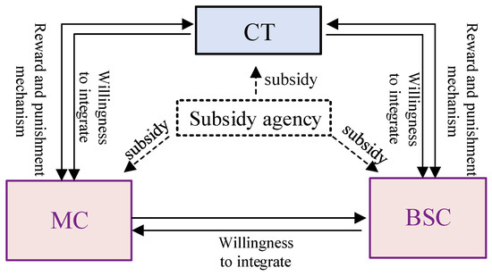
Figure 1.
Game logic relation.
3. Model Hypothesis and Construction
Game theory studies the strategic interactions between rational decision makers, and traditional game theory assumes that participants are perfectly rational. Evolutionary game theory combines game theory and the analysis processes of dynamic evolution, and it assumes that the rationality of participants is finite. In addition, each player can obtain the optimal decision through continuous learning and evolution in the process of evolutionary games. It is difficult for BSC, MC, and CT to determine the optimal strategy in the game, and they adjust their strategies in multiple games. Thus, this paper uses evolutionary game theory to analyze the decision-making behavior among the participants. Before using the evolutionary game model, we make the following four hypotheses.
- (1)
- The participants in the evolutionary game model are BSC, MC, and CT, and the participants are bounded rationally.
- (2)
- The goal of each participant is to achieve maximum benefits. All the participants make decisions by comparing their benefits with others, and they constantly adjust their strategies to achieve eventual equilibrium.
- (3)
- Each participant has two strategies, choosing or not choosing the bicycle–metro integration, which is shown in Table 1. The possibility of BSC choosing the integrated cooperation is x (x ∈ [0,1]), and the possibility of BSC not choosing integrated cooperation is 1 − x. The possibility of MC choosing integrated cooperation is y (y ∈ [0,1]), and the possibility of MC not choosing integrated cooperation is 1 − y. For CT, the probability of choosing integrated cooperation is z (z∈ [0,1]), and the probability of CT not choosing integrated cooperation is 1 − z.
- (4)
- The cooperation between BSC and MC can reduce the cost of the integrated travel mode of sharing bicycles and the metro, and it can increase the number of sharing bicycles and metro travelers. If the integration benefit of BSC or MC is greater than the integration costs, it is profitable for each stakeholder, and the integration model of sharing bicycles and the metro is effective.

Table 1.
The strategies for each player in the evolutionary game.
Table 1.
The strategies for each player in the evolutionary game.
| Player | Expression of Strategies | Strategies |
|---|---|---|
| BSC | Cooperating with MC | |
| Not cooperating with MC | ||
| MC | Cooperating with BSC | |
| Not cooperating with BSC | ||
| CT | Choosing the sharing bicycle–metro integration mode | |
| Not choosing the sharing bicycle–metro integration mode |
The relevant influencing variables are shown in Table 2.
Table 2.
Definitions and assumptions of parameters.
- (1)
- Based on the existing built environment and user demand, is the daily feeder passenger flow of sharing bicycles on the metro station, and is the potential passenger flow of the integrated feeder caused by the shared bicycle–metro integration.
- (2)
- , , and are the surge proportions with different integration cooperation plans. In the case that both BSC and MC choose integrated cooperation, the surge proportion of connecting passenger flow is . When BSC chooses integration while MC does not, the surge proportion of connecting passenger flow is . When MC chooses integration while BSC does not, the surge proportion of connecting passenger flow is (, , ∈ [0,1]).
- (3)
- is the cost when BSC chooses the integration cooperation, including the supervision of CT to park according to the rules and construction of the integrated infrastructure. is the cost when MC chooses the integration, including the supervision of CT to park according to the rules and the construction of the integrated infrastructure.
- (4)
- For the player who chooses integrated cooperation, the subsidy unit will give a certain subsidy fund to motivate the player to choose the integrated mode. is the subsidy fund given to BSC when it chooses integrated cooperation; is the subsidy fund given to MC when it chooses integrated cooperation; is the subsidy fund given to CT when it chooses integrated cooperation.
- (5)
- Set rewards and punishments for the parking behavior of CT, M is the punishment unit price for irregular parking behavior, and Q is the reward unit price for regular parking behavior.
- (6)
- and are the proportions of irregular and regular parking in the connection flow of bicycle sharing, respectively, and .
- (7)
- is the proportion of the distribution of punishment given between BSC and MC. Connecting travelers who park irregularly will be punished. times the fine is attributed to BSC, times the fine is attributed to MC. is the proportion of the distribution of reward given between BSC and MC. Connecting travelers who park regularly will obtain the reward, BSC pays the k2 proportion of the prize, and the other part is paid by MC.
- (8)
- is the unit price of sharing bicycle trips without choosing integration, generally taken as 2 RMB/person. is the unit price of the metro without choosing integration, generally taken as 4 RMB/person.
Based on the assumptions and variable analysis, we can obtain the benefit matrix corresponding to each strategy of the participant. The benefit matrix of BSC, MC, and CT is shown in Table 3.
Table 3.
Strategy benefit matrix for BSC, MC, and CT.
Based on the strategic benefit matrix of multiple participants, the expected benefits of the participants can be obtained. Taking the BSC system as an example, the expected benefit of BSC choosing integrated cooperation is derived from Equation (1).
where is the benefit of BSC under choosing integration strategy. is the strategic benefit of BSC when MC and CT choose integration. is the strategic benefit of BSC when MC does not choose integration and CT chooses integration. is the strategic benefit of BSC when MC chooses integration and CT does not choose integration, and is the strategic benefit of BSC when MC and CT do not choose integration. Therefore, the expression of after finishing is as shown in Equation (2).
In the same way, the expected benefits of the BSC not choosing integrated cooperation are shown in Equation (3).
The average benefit of BSC choosing integrated cooperation and not choosing integrated cooperation is the expected benefit of BSC, which is shown in Equation (4).
Since the decision probabilities of the participants are constantly changing during dynamic evolution, the dynamic evolution equation should be used to reveal the dynamic evolution process of the participant, and the classical method replicates the dynamic equation [38]. Thus, the replication dynamic equation of BSC is as follows.
According to the replication dynamics equation, we can find that their benefits under the different strategies influence the proportion of BSC choosing integrated cooperation. When BSC obtains higher rewards through integrated cooperation than without cooperation, the proportion of BSC choosing cooperation increases, and the value of the increased proportion is linearly related to the difference between the returns of the two strategies. When the expected benefit of BSC choosing integrated cooperation is higher than the average expected benefit of BSC, the willingness of BSC to choose cooperation will increase. Then, the expected benefits and the replication dynamic equations of MC and CT systems can be obtained as follows.
Expected benefits of MC
Replication dynamic equation of MC:
Expected benefits of CT:
Replication dynamic equation of CT:
4. Evolutionary Stable Strategy
4.1. Stable State Analysis
Smith introduced the concept of the evolutionarily stable strategy (ESS) in 1982 [39], which is a strategy adopted by a population in a given environment [40]. Each ESS corresponds to a Nash equilibrium solution, but not all Nash equilibrium solutions belong to the ESS. The probability of a participant choosing a strategy will reach a stable level when the participant cannot obtain higher benefits by changing the strategy, and this strategy is called ESS.
According to evolutionary game theory, the equilibrium point must satisfy the replication dynamic equations , , and , , . The equilibrium points containing strategies of 0, 1 and not 0, 1 are included in the integrated game system of BSC, MC, and CT. The solution process of the equilibrium state is analyzed as follows.
By Equation (6), it is known that x = 0 and x = 1 are the two roots of . There are other roots of that are not 0 and 1.
Case 1: When y = 0, there exists Z1 (see Equation (11)), which makes . If z = Z1 > 0, any decision is in a steady state for the BSC system. If z ≠ Z1, when , there will be and , implying that BSC chooses to cooperate and MC chooses not to cooperate as ESS. When , there will be , , implying that both BSC and MC choose not to cooperate as ESS.
Case 2: When y = 1, there exists Z2 (see Equation (12)), which makes . If , any decision is in a steady state for the BSC system. If , when , there will be and , implying that BSC and MC choose to cooperate as ESS. When , there will be and , implying that BSC chooses not to cooperate while MC chooses to cooperate as ESS.
Case 3: When z = 0, there exists Y1 (see Equation (13)), which makes . If , for the BSC system, any decision is in a steady state. If , when , there will be , , implying that BSC chooses to cooperate while CT chooses not to cooperate as ESS. When 0 < y < Y1, there will be , , implying that neither BSC nor CT choosing not to cooperate as ESS.
Case 4: When z = 1, there exists Y2 (see Equation (14)), which makes . If , for the BSC system, any decision is in a steady state. If , when , there will be , , implying that it is ESS when both BSC and CT choose to cooperate. When 0 < y < Y2, there will be , , implying that the state is ESS when BSC chooses to cooperate while CT chooses not to cooperate.
By Equation (8), it is known that y = 0 and y = 1 are the two roots of . There are other roots of that are not 0 or 1.
Case 5: When = 0, there exists (such as Equation (15)), which makes . If , for the MC system, any decision is ESS. If , when , there will be , , implying that BSC chooses to cooperate while MC chooses not to cooperate is ESS. When , there will be , , implying that the state is ESS when neither BSC nor MC chooses not to cooperate.
Case 6: When x = 1, there exists (such as Equation (16)), which makes . If , any decision is in a steady state for the MC system. If , when , there will be , , implying that it is ESS when BSC and MC choose to cooperate. When , there will be , , implying that the state is ESS when BSC chooses to cooperate while MC does not.
Case 7: When , there exists (such as Equation (17)), which makes . If , any decision is in a steady state for the MC system. If , when , there will be , , implying that it is ESS when MC chooses to cooperate while CT does not. When , there will be , , implying that the state is ESS when neither MC nor CT choose not to cooperate.
Case 8: When , there exists (such as Equation (18)), which makers . If , any decision is in a steady state for the MC system. If , when , there will be , , implying that it is ESS when both MC and CT choose to cooperate. When , there will be , , implying that the state is ESS when CT chooses to cooperate while MC does not.
According to Equation (9), we know that and are the two roots of . There are other roots of that are not 0 or 1.
Case 9: When , there exists (as Equation (19)), which makers . If , any decision is in a steady state for the MC system. If , when , there will be , , implying that it is in a steady state when the BSC chooses to cooperate while CT chooses not to cooperate; when , there will be , , implying that the state is stable when neither BSC nor CT choose not to cooperate.
Case 10: When x = 1, there exists Y4 (as Equation (20)), which makers . If y = Y4 > 0, any decision is in a steady state for the MC system. If y ≠ Y4, when 1 > y > Y4, there will be , , implying that it is ESS when the BSC and CT choose to cooperate. When , there will be , , implying that the state is ESS when BSC chooses to cooperate while CT does not.
Case 11: When y = 0, there exists X3 (as Equation (21)), which makers . If , any decision is in a steady state for the MC system. If , when , there will be , , implying that it is ESS when CT chooses to cooperate while MC does not; when , there will be , , implying that the state is ESS when neither MC nor CT chooses not to cooperate.
Case 12: When y = 1, there exists X4 (as Equation (22)), which makers . If , any decision is in a steady state for the MC system. If , when , there will be , , implying that it is ESS when both MC and CT choose to cooperate. When , there will be , , implying that the state is ESS when MC chooses to cooperate while CT does not.
In addition, eight pure strategy equilibrium points , , , , , , , can be obtained. Since the equilibrium point is not necessarily the optimal ESS, we use the Jacobian matrix to judge the stability of the above points. According to the theory proposed by Taylor and Jonker, the equilibrium point is considered as the ESS of the game if all the eigenvalues of the Jacobian matrix are all negative real parts [41]. The Jacobian matrix of the evolutionary game system in this paper is as follows.
The eigenvalues and stability conditions of the Jacobian matrix at each equilibrium point are shown in Table 4. Each equilibrium point can evolve into a stable strategy, and results can be obtained by adding constraints.
Table 4.
Eigenvalues and stability conditions of the Jacobian matrix.
- (1)
- When the three participants reach the equilibrium point , it means that the benefit of BSC and MC choosing integrated cooperation is greater than the total cost, and the cost of CT choosing the integrated mode is less than the cost of not choosing integrated. Since , , , equilibrium points and , , cannot reach a steady state at the same time.
- (2)
- When the three participants reach the equilibrium point , it means that the benefit of BSC and MC choosing integrated cooperation is less than the total cost, and the cost of CT choosing the integrated mode is greater than the cost of not choosing integrated. Since , , , equilibrium points , , and cannot reach a steady state at the same time.
- (3)
- When the three participants reach the equilibrium point , it means that the benefit of BSC and MC choosing integrated cooperation is less than the total cost, and the travel cost of CT choosing the integrated mode is less than the cost of not choosing integrated. Since , , equilibrium points , and cannot reach a steady state at the same time.
- (4)
- When the three participants reach the equilibrium point , it means that the benefit of BSC choosing integrated cooperation is less than the total cost. The benefit of MC choosing integrated cooperation is greater than the total cost, and the travel cost of CT choosing the integrated mode is greater than the cost of not choosing integrated. Since , , equilibrium points , and cannot reach a steady state at the same time.
- (5)
- When the three participants reach the equilibrium point , it means that the benefit of BSC choosing integrated cooperation is greater than the total cost. The benefit of MC choosing integrated cooperation is less than the total cost, and the travel cost of CT choosing the integrated mode is greater than the cost of not choosing integrated travel. Since , , equilibrium points , and cannot reach a steady state at the same time.
- (6)
- When the three participants reach the equilibrium point , it means that the benefit of BSC choosing integrated cooperation is greater than the total cost. The benefit of MC choosing integrated cooperation is greater than the total cost, and the travel cost of CT choosing the integrated mode is greater than the cost of not choosing the integrated mode.
- (7)
- When the three participants reach the equilibrium point , it means that the benefit of BSC choosing integrated cooperation is greater than the total cost. The benefit of MC choosing integrated cooperation is less than the total cost, and the travel cost of CT choosing the integrated mode is less than the cost of not choosing the integrated mode.
- (8)
- When the three participants reach the equilibrium point , it means that the benefit of BSC choosing integrated cooperation is less than the total cost. The benefit of MC choosing integrated cooperation is greater than the total cost, and the travel cost of CT choosing the integrated mode is less than that of not choosing the integrated mode.
4.2. Solving of Stable Point
Because of the conflict between the equilibrium points in the previous section, when is in equilibrium, , , , and are possibly in equilibrium at the same time. In order to ensure that only is in the equilibrium state, there exists at least one eigenvalue greater than 0. Combined with the actual situation, parameter , . Generally, the proportion of regular parking is greater than that of irregular parking, that is, . In Table 5, we analyze the system’s steady state in three scenarios.
Table 5.
Local stability of the equilibrium state.
Scenario 1:
, . If the reward given to the CT is less than the punishment, the subsidy amount given by the funding organization to the MC and the BSC is greater than the integration cost of BSC and MC, and the subsidy given by the funding organization to the CT is greater than the balance after the reward and punishment; then,is the unique ESS among the eight equilibrium points.
Scenario 2:
, . Unlike Scenario 1, if the subsidy given to the CT by the funding organization is less than the balance after the reward and penalty, then E6 is a unique ESS among the eight equilibrium points.
Scenario 3:
, . Different from Scenario 1, if the reward for CT is greater than the punishment amount, the subsidy for the BSC system and the MC system is reduced, and the subsidy for CT by the funding organization is greater than the balance after the reward and penalty. Then, there are two saddle points and five non-stable points in the eight equilibrium points.
4.3. Active Regulation Effect Based on Policy Factors
To further validate and test the proposed model, this section uses the empirical data to reveal the evolutionary mechanism of the integration system based on the system dynamics simulation method.
The bicycle–metro integration model contains eighteen parameters , , , , , , , , , , , , , , , , , . The initial value settings of the parameters are shown in Table 6. is the average value of shared bicycles connecting metro stations in Beijing. We assume that the maximum connecting surge volume is 500 passengers because of the integration mode. If both BSC and MC are willing to choose integrated cooperation, the surge of connecting passenger flow is . If BSC chooses integrated cooperation while MC does not, the surge connecting passenger flow is . If BSC does not choose integrated cooperation while MC chooses integrated cooperation, the surge of connecting passenger flow is . If BSC and MC do not choose integrated cooperation while CT chooses integrated cooperation, the surge of connecting passenger flow is .
Table 6.
Initial value of parameters.
Since the emergence of sharing bicycles, its development has experienced several booms and fallbacks. From the enormous incentives at the beginning until today, users of sharing bicycles have gradually stabilized. Recently, the sharing bicycle system has set up a punishment mode for irregular parking. Still, this feature has not been commonly enabled due to some disputes caused by inaccurate positioning. Therefore, this section has great significance on the operation of sharing bicycle systems by exploring the reward and punishment penalty policy of parking rules. We set the initial value of irregular parking punishment as 0.5 RMB/person and the initial value of regular parking reward as 0.2 RMB/person.
Due to financial pressures, the subsidies of the funding units will gradually decrease as integration is achieved. The system’s evolution is presented below, in which the subsidy of the three participants decreases with the increase in travelers’ willingness to choose integration cooperation.
Case 1: Let update the replication dynamics equation. The BSC system received a decreasing subsidy as the probability of CT choosing the integration increased. The initial integration intentions of the three participants were set as = 0.3, = 0.4, = 0.5. As shown in Figure 2a–c, with the phasing out of , the dynamic evolutionary trajectory of the three participants shows spiral convergence and the existence of a Nash equilibrium. According to Figure 2d, the dynamic evolutionary trajectory’s fluctuation range gradually decreased and then tended to be stable, but not in the optimal state. The travel willingness under this equilibrium state was around 0.61.
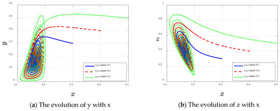
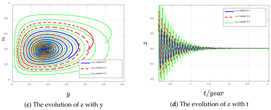
Figure 2.
The dynamic evolution of subsidy policy phasing out.
Case 2: Let . According to Figure 3, the dynamic evolutionary trajectories of the three participants eventually reached equilibrium. The travel willingness of MC under this equilibrium state was 0, and the willingness probability of CT and BSC reached 1.
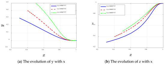
Figure 3.
The dynamic evolution of subsidy policy phasing out.
Case 3: Let . As shown in Figure 4, as the willingness of CT to choose integrated cooperation increased, the willingness of BSC and MC to choose integrated cooperation would be increased and would eventually reach equilibrium. The willingness of each player to choose integrated cooperation was 1, which was the same as the expectations.
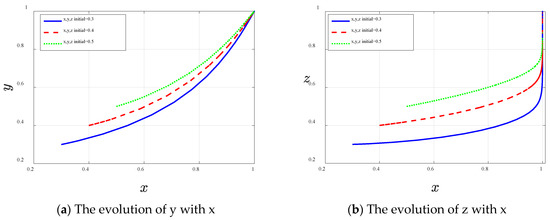
Figure 4.
The dynamic evolution of subsidy policy phasing out.
Therefore, under the mechanism of phasing out the subsidy policy gradually, we focused on how to increase the probability of the ideal event occurring by optimizing the parameter design. According to Figure 5, as the subsidy for BSC decreased, CT did not eventually reach optimal equilibrium. According to Figure 6, as the subsidy for MC decreased, the willingness of BSC to choose integration changed slightly, but when fell to 450, its willingness to choose integration gradually evolved to 0. According to Figure 7, as the subsidy for CT decreased, the integration willingness of MC changed slightly, but when decreased to 200, the cooperation willingness of CT tended to decrease, increase in the initial stage, and finally reach equilibrium. This indicates that there were critical values of , , and to promote the system equilibrium.
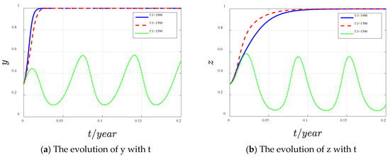
Figure 5.
Active adjustment effect of .
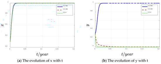
Figure 6.
Active adjustment effect of .
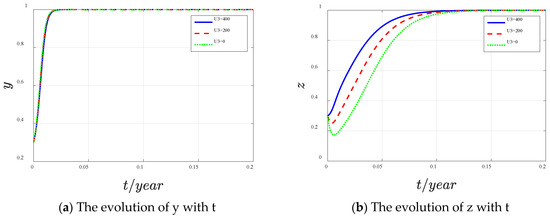
Figure 7.
Active adjustment effect of .
In addition, in terms of the unit price of sharing bicycle and metro trips, we found that the change in the unit price of sharing bicycles had a greater impact on the system equilibrium than the change in metro, by comparing Figure 8a,b. This indicates that the unit price of the sharing bicycle was an important factor affecting the CT’s transportation connection. If the degree of subsidy for CT could dispel their concerns due to the price issues, then the evolutionary game of the three participants would also reach equilibrium. As the irregular parking ratio g1 increased, the CT system reached a steady state that was willing to cooperate more and more slowly through Figure 9a. The continued increase in g1 would eventually lead to the cooperation willingness of CT decreasing to 0. From Figure 9a,b, the change in the irregular parking ratio had little impact on the evolutionary pattern of metro evolution, and the reward and punishment mechanism of irregular parking had more impact on the CT.
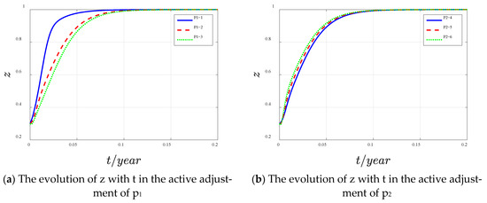
Figure 8.
Active adjustment effect of unit price.
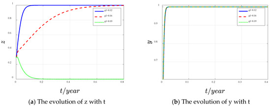
Figure 9.
Active adjustment effect of .
5. Conclusions
The rapid development of bicycle sharing has made the last mile of travel more flexible and efficient for travelers. The bicycle–metro integration mode is a successful way to achieve sustainable urban transport. To promote bicycle–metro integration, this paper used evolution game theory to establish an integration model of a bicycle-sharing system, metro system, and travelers. Combining empirical and sensitivity analyses, the dynamic evolution mechanism of the integration model was explored under the subsidy policy phasing out. The equilibrium state of the integrated system was revealed by actively adjusting the cost factor, subsidy factor, reward and punishment factors, irregularity factor, price factor and passenger flow transfer ratio, and the critical recommended values of factors were obtained. The primary conclusions and management implications are as follows.
Firstly, with subsidy policy phase outs for travelers, the trajectory of the system shows a spiral convergence and then stabilizes. This finding implies that subsidy policy phase outs can more stably promote bicycle–metro integration.
Secondly, the active adjustment response suggests that the unit price of bicycle sharing has a greater impact on the connecting travelers. The integration game model would reach equilibrium if the subsidy to travelers can dispel their concerns due to the price issue. Hence, the bicycle-sharing company should make corresponding efforts toward price design.
Finally, the irregular parking ratio has a greater impact on travelers reaching equilibrium compared to the metro system. It is clear that pushing for a reward and punishment mechanism of irregular parking is important for travelers to choose a bicycle–metro integrated travel mode. Therefore, seeking effective support between policy and participants will be an important future topic for local governments.
The result of this paper is also insightful for promoting bicycle–metro integration across the world. Many researchers argue that a well-integrated system combining public bicycle sharing and metro use could enhance the attractiveness of the metro system [34,42,43,44]. Zhao et al. [43] suggested that future policies should consider ways to encourage people to use bicycles and reside in neighborhoods designed for bicycle–metro integration. Both Yang et al. [44] and Cai et al. [34] studied the system dynamics modeling of dockless bicycle-sharing program operations. However, some real data were not available in their studies. In this paper, as far as possible, we used real data at a quantitative scale to simulate the evolution of the system, which is of practical significance for guiding policy formulation.
There are several limitations to the current study that can be considered as starting points for further research. Firstly, the built environment data were obstacles to exploring more detailed information about the ridership of metro stations and bicycle sharing. The positive effect of better built environments in metro station areas is beneficial to bicycle–metro integration [22]. Secondly, in the process of promotion of the bicycle–metro integration mode, the connection between participants is more complicated. Simultaneous adjusting for multiple policy factors should be considered in future work. Finally, since connections to metro stations include buses and walking in addition to bicycle sharing, multi-model integration is more valuable in promoting the attractiveness of public transportation. Future policies should consider the game between multiple ways of connection to promote bicycle–metro integration.
Author Contributions
Conceptualization, T.C., C.J. and Y.C.; Methodology, T.C., Y.L. and Y.C.; Software, T.C., Y.L. and Y.C.; Validation, C.J., Y.L. and Y.C.; Formal analysis, L.L. and Y.L.; Data collection, C.J., T.C. and Y.L.; Writing—original draft preparation, T.C. and Y.L.; Writing—review and editing, L.L. and Y.C.; Visualization, T.C. and Y.L.; Supervision, all authors. All authors have read and agreed to the published version of the manuscript.
Funding
The research is funded by the National Key Research and Development Program of China (Grant No. 2020YFB1600703).
Conflicts of Interest
The authors declare no conflict of interest. The authors declare no conflict of interest. The funders had no role in the design of the study; in the collection, analyses, or interpretation of data; in the writing of the manuscript, or in the decision to publish the results.
References
- Sun, G.; Zacharias, J. Can bicycle relieve overcrowded metro? Managing short-distance travel in Beijing. Sustain. Cities Soc. 2017, 35, 323–330. [Google Scholar] [CrossRef]
- Lin, D.; Zhang, Y.; Zhu, R.; Meng, L. The analysis of catchment areas of metro stations using trajectory data generated by dockless shared bikes. Sustain. Cities Soc. 2019, 49, 101598. [Google Scholar] [CrossRef]
- Fishman, E.; Washington, S.; Haworth, N.; Mazzei, A. Barriers to bikesharing: An analysis from Melbourne and Brisbane. J. Transp. Geogr. 2014, 41, 325–337. [Google Scholar] [CrossRef]
- Davis, L.S. Rolling along the last mile: Bike-sharing programs blossom nationwide. Planning 2014, 80, 10–16. [Google Scholar]
- Demaio, P. Bike-sharing: Its History, Models of Provision, and Future. J. Public Transport. 2009, 12, 3. [Google Scholar] [CrossRef]
- Fishman, E. Bikeshare: A review of recent literature. Transp. Rev. 2016, 36, 92–113. [Google Scholar] [CrossRef]
- Parkes, S.D.; Marsden, G.; Shaheen, S.A.; Cohen, A.P. Understanding the diffusion of public bikesharing systems: Evidence from Europe and North America. J. Transp. Geogr. 2013, 31, 94–103. [Google Scholar] [CrossRef]
- Shen, Y.; Zhang, X.; Zhao, J. Understanding the usage of dockless bike sharing in Singapore. Int. J. Sustain. Transp. 2018, 12, 686–700. [Google Scholar] [CrossRef]
- Chen, Z.; Lierop, D.V.; Ettema, D. Dockless bike-sharing systems: What are the implications? Transp. Rev. 2020, 40, 333–353. [Google Scholar] [CrossRef]
- Zhang, L.; Zhang, J.; Duan, Z.Y.; Bryde, D. Sustainable bike-sharing systems: Characteristics and commonalities across cases in urban China. J. Clean. Prod. 2015, 97, 124–133. [Google Scholar] [CrossRef]
- Du, Y.; Deng, F.; Liao, F. A model framework for discovering the spatio-temporal usage patterns of public free-floating bike-sharing system. Transp. Res. Part C Emerg. Technol. 2019, 103, 39–55. [Google Scholar] [CrossRef]
- Ma, G.; Zhang, B.; Shang, C.; Shen, Q. Rebalancing Stochastic Demands for Bike-sharing Networks with Multi-scenario Characteristics. Inf. Sci. 2020, 554, 177–197. [Google Scholar] [CrossRef]
- Yang, L.; Zhang, F.; Kwan, M.P.; Wang, K.; Zuo, Z.; Xia, S.; Zhang, Z.; Zhao, X. Space-time demand cube for spatial-temporal coverage optimization model of shared bicycle system: A study using big bike GPS data. J. Transp. Geogr. 2020, 88, 102861. [Google Scholar] [CrossRef]
- Sun, S.H. The spatial spread of dockless bike-sharing programs among Chinese cities. J. Transp. Geogr. 2020, 86, 102782. [Google Scholar]
- Martens, K. The bicycle as a feedering mode: Experiences from three European countries. Transp. Res. Part D Transp. Environ. 2004, 9, 281–294. [Google Scholar] [CrossRef]
- Rietveld, P.; Daniel, V. Determinants of bicycle use: Do municipal policies matter? Transp. Res. Part A Policy Pract. 2004, 38, 531–550. [Google Scholar] [CrossRef]
- Singleton, P.A.; Clifton, K.J. Exploring Synergy in Bicycle and Transit Use. Transp. Res. Rec. J. Transp. Res. Board 2014, 2417, 92–102. [Google Scholar] [CrossRef]
- Guo, Y.; Yang, L.; Lu, Y.; Zhao, R. Dockless bike-sharing as a feeder mode of metro commute? The role of the feeder-related built environment: Analytical framework and empirical evidence. Sustain. Cities Soc. 2020, 65, 102594. [Google Scholar] [CrossRef]
- Guo, Y.; Yang, L.; Huang, W.; Guo, Y. Traffic Safety Perception, Attitude, and Feeder Mode Choice of Metro Commute: Evidence from Shenzhen. Int. J. Environ. Res. Public Health 2020, 17, 9402. [Google Scholar] [CrossRef]
- Keijer, M.J.N.; Rietveld, P. How do people get to the railway station The dutch experience. Transp. Plan. Technol. 2000, 3, 215–235. [Google Scholar] [CrossRef]
- Wang, R.; Liu, C. Bicycle-Transit Integration in the United States, 2001–2009. J. Public Transp. 2013, 3, 95–119. [Google Scholar] [CrossRef]
- Puello, L.L.P.; Geurs, K.T. Modelling observed and unobserved factors in cycling to railway stations: Application to transit-oriented-developments in the Netherlands. Delft Univ. Technol. 2015, 15, 27–50. [Google Scholar]
- Zhou, S.; Ni, Y. Effects of Dockless Bike on Modal Shift in Metro Commuting: A Pilot Study in Shanghai. In Proceedings of the Transportation Research Board 97th Annual Meeting, Washington, DC, USA, 7–11 January 2018. [Google Scholar]
- Martens, K. Promoting bike-and-ride: The Dutch experience. Transp. Res. Part A Policy Pract. 2007, 41, 326–338. [Google Scholar] [CrossRef]
- Ji, Y.; Fan, Y.; Ermagun, A.; Cao, X.; Wang, W.; Das, K. Public bicycle as a feeder mode to rail transit in China: The role of gender, age, income, trip purpose, and bicycle theft experience. Int. J. Sustain. Transp. 2017, 11, 308–317. [Google Scholar] [CrossRef]
- Liu, L.; Sun, L.; Chen, Y.; Ma, X. Optimizing fleet size and scheduling of feeder transit services considering the influence of bike-sharing systems. J. Clean. Prod. 2019, 236, 117550. [Google Scholar] [CrossRef]
- Ricci, M. Bike sharing: A review of evidence on impacts and processes of implementation and operation. Res. Transp. Bus. Manag. 2015, 15, 28–38. [Google Scholar] [CrossRef]
- Purtik, H.; Arenas, D. Embedding Social Innovation: Shaping Societal Norms and Behaviors Throughout the Innovation Process. Bus. Soc. 2019, 58, 963–1002. [Google Scholar] [CrossRef]
- Jia, L.; Xin, L.; Liu, Y. Impact of Different Stakeholders of Bike-Sharing Industry on Users’ Intention of Civilized Use of Bike-Sharing. Sustainability 2018, 10, 1437. [Google Scholar] [CrossRef]
- Sun, Y. Sharing and Riding: How the Dockless Bike Sharing Scheme in China Shapes the City. Urban Sci. 2018, 2, 68. [Google Scholar] [CrossRef]
- Gu, T.; Kim, I.; Currie, G. To be or not to be dockless: Empirical analysis of dockless bikeshare development in China. Transp. Res. Part A Policy Pract. 2019, 119, 122–147. [Google Scholar] [CrossRef]
- Hollander, Y.; Prashker, J. Applicability of non-cooperative game theory in transport systems analysis. Transportation 2006, 33, 481–496. [Google Scholar]
- Sun, L.J.; Gao, Z.Y. An equilibrium model for urban transit assignment based on game theory. Eur. J. Oper. Res. 2007, 181, 305–314. [Google Scholar] [CrossRef]
- Cai, J.; Liang, Y. System Dynamics Modeling for a Public–Private Partnership Program to Promote Bicycle–Metro Integration Based on Evolutionary Game. Transp. Res. Rec. J. Transp. Res. Board 2021, 2675, 689–710. [Google Scholar] [CrossRef]
- Wang, Z.; Zheng, L.; Zhao, T.; Tian, J. Mitigation strategies for overuse of Chinese bikesharing systems based on game theory analyses of three generations worldwide. J. Clean. Prod. 2019, 227, 447–456. [Google Scholar] [CrossRef]
- Beijing Transport Institute. 2013 Beijing Annual Transport Development Report. 2014. Available online: https://www.bjtrc.org.cn/List/index/cid/7.html (accessed on 25 September 2022).
- Feng, X.; Saito, M.; Wang, Q. Reducing average comprehensive travel cost by rationally allocating trips to different travel modes. Transp. Plan. Technol. 2017, 40, 679–688. [Google Scholar] [CrossRef]
- Hauer, J.F.; Trudnowski, D.J.; Rogers, G.; Mittelstadt, B.; Johnson, J. Evolutionary games and population dynamics. IEEE Comput. Appl. Power 1998, 10, 50–54. [Google Scholar] [CrossRef]
- Smith, J.M. Evolution and the Theory of Games; Cambridge University Press: Cambridge, UK, 1988. [Google Scholar]
- Jiang, X.; Ji, Y.; Du, M.; Wei, D. A Study of Driver’s Route Choice Behavior Based on Evolutionary Game Theory. Comput. Intell. Neurosci. 2014, 2014, 47. [Google Scholar] [CrossRef]
- Taylor, P.D.; Jonker, L.B. Evolutionarily Stable Strategies and Game Dynamics. Math. Biosci. 1978, 40, 145–156. [Google Scholar] [CrossRef]
- Shaheen, S.; Guzman, S.; Zhang, H. Bikesharing in Europe, the Americas, and Asia. Transp. Res. Rec. J. Transp. Res. Board 2010, 2143, 159–167. [Google Scholar] [CrossRef]
- Zhao, P.; Li, S. Bicycle-metro integration in a growing city: The determinants of cycling as a transfer mode in metro station areas in Beijing. Transp. Res. Part A Policy Pract. 2017, 99, 46–60. [Google Scholar] [CrossRef]
- Yang, T.; Li, Y.; Zhou, S. System Dynamics Modeling of Dockless Bike-Sharing Program Operations: A Case Study of Mobike in Beijing, China. Sustainability 2019, 11, 1601. [Google Scholar] [CrossRef]


Publisher’s Note: MDPI stays neutral with regard to jurisdictional claims in published maps and institutional affiliations. |
© 2022 by the authors. Licensee MDPI, Basel, Switzerland. This article is an open access article distributed under the terms and conditions of the Creative Commons Attribution (CC BY) license (https://creativecommons.org/licenses/by/4.0/).