Article

Can Renewable Energy and Export Help in Reducing Ecological Footprint of India? Empirical Evidence from Augmented ARDL Co-Integration and Dynamic ARDL Simulations

1
Vinod Gupta School of Management, Indian Institute of Technology, Kharagpur 721302, India
2
School of Business, University of Petroleum and Energy Studies, Dehradun 248007, India
3
Department of Agricultural Finance and Banking, Bangladesh Agricultural University, Mymensingh 2202, Bangladesh
*
Authors to whom correspondence should be addressed.
Sustainability 2022, 14(23), 15494; https://doi.org/10.3390/su142315494
Submission received: 20 October 2022 / Revised: 12 November 2022 / Accepted: 18 November 2022 / Published: 22 November 2022
(This article belongs to the Special Issue Ecological Transition and Circular Economy)

Abstract

:
The objective of this study is to investigate the impact of exports, renewable energy, and industrialization on the ecological footprint (EF) of India over the period spanning from 1970–2017 by employing the newly developed augmented ARDL (A-ARDL) co-integration approach and the novel dynamic ARDL (D-ARDL) technique. The empirical results demonstrate that exports and renewable energy consumption reduce the EF, while industrialization intensifies the EF. More precisely, a 1% increase in export (renewable energy consumption) reduces the EF by 0.05% (0.09%). In addition, the short-run elasticity of the GDP is found to be larger than the long-run elasticity indicating the possibility of the existence of the Environmental Kuznets Curve (EKC) of the EF for India. The study indicates that the income effect and increased policy focus on renewable energy usage can be expected to reduce India’s per capita EF in the long run. Moreover, India’s export sector has been traditionally less energy intensive, which reflects in our findings of export growth leading to a reduction in EF. Based on the empirical findings, this study recommends some policy insights that may assist India to effectively reduce its ecological footprint.

1. Introduction

In the contemporary period, controlling greenhouse gas emissions and mitigating climate change is the pivotal policy agenda around the globe and one of the pioneering goals under the United Nations Sustainable Development Goals (SDG-13) [1,2,3]. While global commitment is to reduce the world’s average increase of temperature below 1.5 °C, India is not an exception, and is obligated toward net zero emissions by 2070. Moreover, India, the second most populated country of more than 1.2 billion has emerged as one of the most important markets in the world, with the third largest GDP in terms of purchasing power parity. According to World Bank estimates, India is also expected to be one of the fastest-growing economies, with a growth percentage of 6–7% in the coming decade. This enormous amount of growth, however, comes with immense natural resource costs. The natural resources available to a country take time to regenerate but can be used up in no time, and hence, a country’s growth is unlikely to be sustainable for future generations if the rate of its resource usage is much higher than the rate of the regeneration of those resources. Thus, the balance between resource usage and the ecological capacity to replenish them, i.e., biocapacity, is imperative for the sustainable development of any economy. The Global Footprint Network pioneered the process of systematic measurement and accounting of an ecological footprint in 2003, in order to trace anthropogenic usage of ecosystems in comparison to a renewal of those ecosystems. This is done every year to keep track of the economy’s demand on the environment and to assess its sustainability.
The total demand of an economy from nature can be in the form of forests and fisheries and cropping and grazing land that is either converted into various kinds of infrastructure for people or can be used to absorb waste generated from various economic activities. The total of these two usages represents an economy’s ecological footprint. If the economy’s footprint exceeds its biocapacity, there is an “ecological overshoot”, which indicates an unsustainable economic growth path [4]. As shown in Figure 1, the ecological deficit of India has been widening since 1980, when the deficit was around 56% of the biocapacity of the country. The gap increased to around 100% at the beginning of the new millennium and was more than 170% in 2018. It needs to be noted here that the consistent overshoot of ecological consumption in the 1990s coincided with economic liberalization and the opening up of the economy, and the distinct widening of the gap in the 2000s, as evident from Figure 1, coincided with the newfound economic prosperity of the country with the worldwide boom in the IT sector.
Most of the climate literature in social sciences has, until date, focused primarily on the nexus between economic growth, in the form of GDP, and carbon emissions, caused primarily by the anthropogenic consumption of energy [5,6]. However, while carbon emissions are an important GHG, the issue of climate change is too complex to just account for anthropogenic carbon emissions in isolation. The dynamic change in the depletion of the natural resource space in totality vis a vis the economic growth that it is contributing to, the environment needs to be examined together to understand if an economy is moving towards sustainability or away from it. Economic growth in turn is also not uniform, and the various components of the GDP contribute in different ways to the various economic activities that impose their demand on natural resources. One such important component is exports, and this study attempts to find the impact of exports on the change in the ecological footprint (EF) of India. India’s rapid economic growth, especially in the post-liberalization era has been accompanied by substantial growth in exports, with the share of exports in total GDP going up to 20.8% in 2021. The share of merchandise export in total GDP increased from 11.4% in 2017 to 13.3% in 2021–2022 [7].
It is well established in the literature that exports not only contribute to a direct increase in the GDP of a country but also contribute to the growth and development of a country through specialization, productivity increase, improved technology and R&D, economies of scale, the expansion of associated industries and service sections, and the employment and income generation that leads to a better standard of living [8,9]. However, this expansion in economic activity through production and consumption rise in a country cannot be fulfilled without drawing from the environment and using up natural resources, land area, and water bodies nor without the emission of pollutants that need land cover for adequate absorption. Moreover, the extent of the export sector’s demand on ecology would be dependent on the nature of the export goods. Hence, in the context of the sustainability of export-led growth—or even growth leading to higher exports—it is imperative to understand its impact on the ecological footprint.
While there are some studies on the impact of trade and export diversification on the environment, as discussed in detail in the next section, there are not many studies that have explored the link between exports as part of GDP and the environment. The export sector, being the comparative advantage of an economy, can be assumed to be more efficient than most other sectors of the economy and is likely to attract more investments and eventually expand more. Hence, it is important to link exports, per se, with the EF of a country without considering imports like in variables like trade openness, which may not have any direct impact on the ecological balance of an economy.
It is also known that the industrialization of an economy raises the demand on the ecology through increased energy and land, water, and natural resource consumption as well as the higher production of pollutants. The higher penetration of renewable energy usage in both production and consumption sectors is likely to impact biodiversity usage also. India’s commitment to integrating the UN Sustainable Development Goals into its economic growth path has led to a rapid expansion of its renewable energy sector. The installed capacity of renewable energy grew by almost 286% over the past 7.5 years, and today, India ranks fourth in overall renewable energy capacity in the world [10].
Consequently, a vast number of studies in the existing body of climate literature provide immense attention to studying the influence of export and industrialization in the pathway of environmental correction. While the sustainable growth of any economy has been highly reliant on the expansion of export and industrial development, the extant literature provides mixed outcomes while examining their influence on ecological corrosion. While various studies in the existing body of knowledge articulate the beneficial impact of exports in attaining ecological correction [11,12], Rahman et al. [13] and Gozgor and Can [14] refuted the former argument and provided the detrimental association of exports in attaining ecological fortification. In addition, while various studies investigate the influence of industrialization in the carbon neutralization of India [15,16], such investigation on an ecological footprint solely for India has been missing in the existing body of knowledge.
Against this milieu, this research has been expected to add novel contributions to the existing body of knowledge in the following ways by utilizing 48 years of annual time series data from 1970–2017: (i) in contrast to the earlier empirical investigations, this study utilizes ecological footprint as a proxy of an environmental quality indicator for India and investigates the dynamic association among the ecological footprint, exports, renewable energy consumption, industrialization, and GDP. (ii) To the best of our knowledge, this is the first study that investigates the impact of exports on the ecological footprint, specifically for India. (iii) While the existing body of the Environmental Kuznets Curve (EKC) literature available for India fails to provide any specific shape of the EKC for India, this study finds evidence of the EKC of ecological footprints for India in the existing framework. (iv) Employing an augmented ARDL (A-ARDL) co-integration technique to overcome the degeneracy problems and shortcomings of the classical ARDL cointegration model in the existing framework is a novel contribution. (v) Finally, the application of a dynamic ARDL simulation and Breitung and Candelon’s (2006) spectral causality test is expected to provide a robust policy-oriented outcome in the existing framework.
The paper is organized as follows—Section 2 provides a literature review on earlier studies; Section 3 describes the data and methodology used in the study; Section 4 is on results and their discussions; and Section 5 concludes with the policy implications of inferences made from the empirical analyses.

2. Literature Review

2.1. Renewable Energy and Environment

Most nations have been focusing on cleaner energy supplies in order to achieve sustainable economic development while not harming the environment, as the substantial usage of non-renewable energy is discovered to be more carbon-intensive [17]. It cannot be refuted that using REC might worsen environmental degradation in this case [18]. However, the influence of REC on climate change is less destructive and more affordable when compared to non-renewable energy [19,20]. Sharma et al. [21], Inglesi-Lotz and Dogan [22], and Dogan and Seker [23] also found that using REC is substantially more ecologically friendly over time.
The surveillance of air, water, and land conditions has also evolved, in addition to CO2 emissions, since it is impossible to ignore how negatively economic activity affects these natural parameters [24]. In this sense, the EF has come into action and plays an important role in terms of environmental quality measurement among academics and researchers. Similar to the reasons that cause CO2 emissions, a number of economic, societal, and political factors affect the EF. Researchers believe that cleaner technology and renewable power sources cause environmental degradation to decline [25]. The impact of using fossil fuels and renewable energy on the ecosystem has been examined by Sharif et al. [26] for 74 economies between 1990 and 2015 and demonstrates that the use of green energy does have a negative coefficient. Bello et al. [27] looked at the environmental impacts of Malaysia’s hydroelectric energy consumption from 1971 to 2016. They discovered that the usage of hydroelectric electricity decreased environmental damage. According to Ben Jebli et al. [28], REC improves the environment in 22 nations in Central and South America over the long term. In order to revisit the effects of REC and non-renewable energy usage on Turkey’s EF, Sharif et al. [29] used the QARDL approach for the years 1965Q1–2017Q4. The results revealed that REC has a long-term negative impact on each quantile of the EF. Christoforidis and Katrakilidis [30] for OECD countries follow a similar line. Xue et al. [31] have also concluded the favorable influence of adopting renewable energy penetration on the EF of four South-Asian nations over the data period 1990–2014. Similar findings has also been evidenced by Dogan and Shah [32] for GCC economies, and by Kim [33] for South Korea.
A few studies have also been done in the instance of India regarding REC and environmental quality; however, most of them use CO2 emissions as a stand-in for environmental quality rather than EF. For instance, Akadiri and Adebayo [34] examined these correlations utilizing annual data spanning from 1970 to 2018 using a variety of econometric techniques. The findings showed that carbon emissions in India are decreased by favorable changes in the REC. It is now even more crucial to look at the function of the REC for India, as Rej and Nag [35] discovered evidence of an N-shaped EKC for CO2 emissions for India with a potential policy divergence between capital generation and REC penetration in the economy. As a result, there is a glaring research vacuum when it comes to evaluating the relationship between REC and the environment, while using EF as a stand-in for environmental conditions in India.

2.2. Export and Environmental Quality

Trade openness, which is determined by the proportion of total exports to imports in the GDP, is a typical way to depict international trade in previous empirical investigations [36]. However, in addition to trade openness, the international trade basket’s makeup can have a significant impact on environmental quality [37]. As a result, subsequent studies have evaluated the environmental effects of international trade by using the value of export items (or concentration) as a percentage of the GDP to reflect the makeup of the global trade portfolio. Conflicting views on how diversifying the export mix would affect the environment have been supported by prior empirical studies. Export diversification has been linked to increased environmental degradation in certain studies [38,39], but it has also been shown to improve the quality of the environment [40,41]. In a similar vein, trade openness has also shown either positive or negative effects on the environmental quality, depending on the industrialization and development level of a country [42]. For instance, to examine the link between EF and trade openness in Qatar, Charfeddine [43] discovered a two-way causal relationship between EF and total foreign trade. Alola et al. [44] found that trade openness had a negative influence on the EF in the European region; as a result, it had a positive effect on environmental quality.
In another view, Hu et al. [45] found that exports and imports have a positive effect on the EF. According to Dogan et al. [46], urbanization promotes environmental pollution at the upper quantiles, and so does export quality, based on the nations’ wealth levels. Rahman [47] came to a similar conclusion on the negative linkage between exports and the states of the environment. Contrarily, in their analysis of the relationship between export product concentration and CO2 emissions in 19 industrialized economies, Apergis et al. [11] came to the conclusion that greater levels of export product concentration result in reduced CO2 emissions. There has not been consensus on this relationship, though, which gives scholars more space to delve deeper into this area of environmental economics.
Scholars have underlined that the export content is just as pertinent as the export volume [48]. Export attributes are influenced by structural change, particularly in nations that are in the middle of their economic development [49]. The development of competitive advantages through the production of higher-quality versions of existing items boosts productivity and export earnings, which in turn encourages the export of environmentally friendly goods. The diversification of new goods is a must for making significant progress in quality improvement for developing nations like India. These show that increasing exports is a crucial policy concern, and they are backed up by instances from developed nations that have been successful in accomplishing structural improvements in terms of both the economy and the environment through the improvement of export quality. However, since its big export volume necessitates considerable resource exploitation, India, a major exporter, has so far received less attention in the analysis of the environmental effect of its export volume. As a result, there is still a significant knowledge gap regarding the nexus between exports and the environment in India. This gap would be filled by this research, as well as contribute to the body of existing literature.

2.3. Industrialization and Environmental Quality

The causality between industrialization and environmental quality has been intensively studied in this era of industrialization development. Alam [50] looked at how selected South Asian nations’ GDP value addition in the service, industrial, and agricultural sectors affected their CO2 emissions. The results of this study revealed that whereas industrial and service value-added have favorable significant impacts on CO2 emissions, agricultural value-added has a negative influence on CO2 emissions. In the Chinese economy, Huan et al. [51] look at the connection between industrial productivity and environmental quality. The findings supported the existence of a long- and short-term N-shaped relationship between these variables in China. The results also provide two industrial output thresholds for environmental quality. The highest threshold point of industrial output is 29.21%, at which the quality of the environment is getting worse off, and the lower threshold point is 30.71%, at which the quality of the environment turns out to be good in the long run in China. Using ARDL and VECM, Liu and Bae [52] examined the impact of IVA on CO2 emissions in China. The study discovered that IVA increases CO2 emissions while causality findings revealed that long-term feedback occurs between them. In 69 nations, Liu and Hao [53] used the FMOLS and DOLS techniques to confirm the existence of a positive association between IVA and CO2 emissions. Using the dynamic ARDL simulation model, Hossain et al. [15] examined the relationship between IVA and CO2 emission in India and found that when income and IVA grow, environmental quality declines as a result of rising CO2 emissions.
In addition, a threshold regression model was used by Dong et al. [54] to assess the effects of urbanization and industrialization on carbon emissions in 14 developed nations. Industrialization increases carbon emissions from the standpoint of income levels. Industrialization progressively has a positive impact on carbon emissions, especially at low- and middle-income levels. However, at the high-income level, this promotional impact starts to wane. Using a nonlinear ARDL model, Ullah et al. [55] tried to establish the link between industrialization and CO2 emissions in Pakistan over the years 1980–2018. The findings show that industrialization raises emissions, whereas deindustrialization lowers emissions over the long and short terms and subsequently improves the environmental quality. In a sample of 44 Sub-Saharan African nations over the years from 2000–2015, Mentel et al. [56] sought to investigate the connection between industrial value added, renewable energy, and CO2 emissions. They discovered that the proportion of industry in GDP has a considerable beneficial influence on CO2 emissions using a two-step system GMM estimator. However, Appiah et al. [57] showed that over the long run, fossil fuel use, industrialization, and urbanization had a non-significant beneficial effect on CO2 emissions for SSA nations.
Interestingly, according to Yang and Khan’s [58] research, capital creation and industrial value-added (IVA) increase environmental sustainability in IEA member nations. Similarly, IVA massively increases CO2 emissions over the short term while boosting the environmental quality in the long term, according to research by Abbasi et al. [59]. Khan [60] asserts that despite China’s primary industries’ decreased CO2 emissions, the secondary and tertiary sectors continue to have a beneficial relationship with one another. The discussion above indicates that there is disagreement over the impact of IVA on the environment, as there are diverse findings on this nexus reported by the researchers. However, the impact of IVA on EF in the context of India is concerning. Thus, the focus of this study was on the influence of IVA on the EF in the setting of India, where it is grave and requires in-depth investigation.

2.4. Economic Development and Environmental Quality

Numerous studies have looked at the nexus between environmental quality and economic growth (GDP) in light of the Environmental Kuznets Curve (EKC) hypothesis. As the economy reaches a specific level of per-capita income and reaches economic maturity, it is projected that the connection between the GDP and CO2 emissions would take the shape of an inverted U. The EKC and curve shape utilizing CO2 emissions have been the subject of extensive investigation and found diluted results. For instance, in their study, Shahbaz et al. [61] examined the impact of the GDP on carbonization in Tunisia from 1971 to 2010, when EKC was still operational in that country. They found that the connection between carbonization and GDP was inverted U-shaped. Furuoka [62] investigated the relationship between the GDP and CO2 emissions using the EKC model; however, there was no proof of an EKC between the two. The association between environmental destruction and GDP in EU countries was examined in the study of [63]. A one-way association between the GDP and CO2 was discovered by the study. Gyamfi et al. [64] used data from 1995 to 2018 to create their N-shaped EKC research for the E7 countries.
In 35 OECD countries, between 2000 and 2014, Ozcan et al. [65] discovered that economic development and energy consumption patterns improve countries’ environmental performance levels. The EKC only exists in the long term, according to Shahbaz et al. [66], who used a sample of Vietnam’s yearly data from 1974 to 2016 to make this discovery. The link between long-term income and pollution is, however, best captured by the N-shape. This suggests that, during a certain stage of economic expansion, Vietnam might anticipate a brief decrease in CO2 emissions. However, after reaching another income tipping point, this will be followed by an additional increase in CO2 emissions. In the long run, economic growth and environmental deterioration are linked in the BRICS nations, according to Naseem et al. [67]. On the other hand, Rahman et al. [68] discovered a high correlation between environmental degradation and economic development, but were unable to detect EKC in the BRICS region.
Other researchers have also used the EF as a proxy of environmental pollution and reported the shape of the relation between EF and GDP. According to Danish et al. [69], economic expansion results in a larger ecological footprint, which exacerbates environmental deterioration. The connections between natural resources, technical advancements, GDP, and the consequent EF in rising nations were examined by Ahmad et al. [70]. Long-term growth and the expansion of the EF are driven by natural resources and GDP, while technology advancements assist in slowing down environmental deterioration. Furthermore, in the context of the EKC hypothesis, the quadric term of GDP had a negative influence on the EF. Similar findings for other nations and the economic bloc have also been reported in other research [71]. Additionally, some study on this connection was done in India [72]. In India, Ahmed and Wang [73] discovered an inverted U-shaped relationship between the GDP and EF. According to Murshed et al. [74], it is essential to foster intra-regional trade and hasten economic expansion if South Asian countries are to significantly reduce their EFs. Additionally, for the South Asian panel, as well as for Bangladesh, Sri Lanka, Nepal, and Bhutan, the results confirm the EKC hypothesis, but not for India and Pakistan. Economic growth has a favorable long- and short-term impact on EF, according to Adebayo et al. [75], who also supported the EKC theory in India.

3. Data Definition and Empirical Approach

This section entails the detailed data description and empirical strategy adopted for obtaining robust policy-oriented outcomes.

3.1. Data Description

This research exploits 48 years of annual time series data from 1970–2017 to investigate the influence of GDP, export, industrialization, and aggregate renewable energy deployment on the EF of India. For this multivariate time series analysis, we have included the following variables: EF in global hectares/capita as the proxy of environmental decay, real GDP per capita in constant 2015 USD as a proxy of economic prosperity, industry value added (% of GDP) as a proxy of industrialization, export of goods and services (% of GDP), and REC in tonnes of oil equivalent/capita. The data for GDP, exports, and industrialization have been outsourced from World Development Indicator (WDI). EF data has been outsourced from the Global Footprint Network. REC data has been taken from the BP Statistical Review of World Energy. Further, the data sources with a detailed explanation have been outlined in Table 1. The descriptive measures of the variables, as shown in Table 2, say that all the variables except IVA are right-skewed. All the variables seem to follow a normal distribution. EF seems to have a very strong positive association with GDP and exports, a moderate association with IVA, and a very strong negative linkage with REC.

3.2. Empirical Strategy

Before beginning an econometric study, it is essential to look at the stationary qualities of the time series variables to prevent unneeded regression problems. We have used the traditional unit root tests, i.e., Augmented Dickey–Fuller (ADF) and the Phillips–Perron (PP) tests to serve that purpose. However, traditional unit root tests have been criticized for having low power to reject the null hypothesis in the presence of a structural break. The second generation unit root test technique, i.e., Zivot and Andrews (1992) structural break unit root test, has been done additionally to determine the break date. Traditional co-integration techniques, i.e., Engle–Granger [76], and Johansen–Juselius [77] require all the variables to be integrated into I(1). The frequently used ARDL bounds test of the co-integration approach, developed by Pesaran et al. [78], requires the independent variables to be integrated at I(1) or fractionally integrated to I(0)/I(1) under the assumptions that the dependent variable needs to be stationary at first differenced form. McNown et al. [79] and Sam et al. [80] counter-argued that in many of the research articles, one of the pre-conditions of applying the ARDL bounds testing approach, i.e., the dependent variable needs to be integrated at I(1) has not been followed. The augmented ARDL (A-ARDL) bounds test co-integration approach, proposed by McNown et al. [79], overcomes the critics of the ARDL bounds test co-integration approach, developed by Pesaran et al. [78]. This model allows the variables to be integrated in any order other than integrated to I(2). The augmented ARDL model under log-linear specification can be presented as follows:
Δ l n E F t = ϕ 0 + γ 1   D U t + ϕ 1   l n E F t 1 + ϕ 2   l n G D P t 1 + ϕ 3   l n E X P t 1 + ϕ 4   l n I V A t 1 + ϕ 5   l n R E C t 1 + j = 1 k 1   β 1 j Δ l n E F t j + j = 0 k 2   β 2 j   Δ l n G D P t j + j = 0 k 3   β 3 j Δ l n E X P t j + j = 0 k 4   β 4 j Δ l n I V A t j + j = 0 k 5   β 5 j Δ l n R E C t j + ε 1 t
In Equation (1), the first difference operator has been denoted by ∆, γ1 is the coefficient of the break dummy variable, the lag accompanied with each of the variables have been represented by k1k5, the nomenclature of the variables is the same as given in Table 1, ln represents the logarithmic transformation of the variables, the summation term captures the short run coefficients, and ε 1 t represents the white noise error term.
The bound F test has been performed by considering the optimal lag structure through Akaike Information Criteria (AIC) statistics and setting the null hypothesis of the lagged term of variables to zero (i.e., H0: ϕ1 = ϕ2 = ϕ3 = ϕ4 = ϕ5 = 0). The cointegrating situation has arrived if the estimated Foverall surpasses the upper bound critical values designed by Narayana [81]. This model is also capable of eliminating the degeneracy problem that arises in the case of the ARDL bounds testing approach. In the ARDL bounds testing approach, two degeneracy cases may arise: (i) lagged explanatory variables are not statistically significant, and (ii) lagged level of the outcome variable is not statistically significant. In order to address these degeneracy issues, McNown et al. [79] and Sam et al. [80] have proposed two additional tests in the existing ARDL bounds testing framework: (i) examining the significance level of the lagged dependent variable through a t-test (tDV) by setting the null hypothesis, (H0: ϕ1 = 0) and a cointegration situation is feasible if the estimated tDV is greater than the upper bound critical values computed by Pesaran et al. (2001); (ii) investigating the significance level of the lagged independent variables through the F test (FIDV) by setting null hypothesis H0: ϕ2 = ϕ3 = ϕ4 = ϕ5 = 0 and cointegration situation can be reached if the estimated FIDV surpasses the upper bounds critical values designed by Sam et al. [81].
After having the confirmation of long-run co-integration among the core variables, the dynamic ARDL technique (D-ARDL), proposed by Jordan and Philips [68], has been employed to compute the long and short-run coefficient estimates. The D-ARDL technique can be considered as a superior technique over the classical ARDL model in case of low convergence speed, and the variables can be integrated into any order except I(2) [82]. The DARDL can also construct graphs showing positive and negative counterfactual adjustments in independent variables and their influence on dependent variables, which is not facilitated in the classical ARDL approach [82,83,84]. The D-ARDL model in our present study can be expressed as follows:
( l n E F ) t = λ 0 + θ 0 l n E F t 1 + β 1 Δ l n G D P t + θ 1 l n G D P t 1 +       β 2 Δ l n E X P t + θ 2 l n E X P t 1 + β 3 Δ l n I V A t + θ 3 l n I V A t 1 + β 4 Δ l n R E C t + θ 4 l n R E C t 1 + ξ E C T t 1 + u t
The classical D-ARDL technique helps in the computation of the short and long-run influence of the determinants on EF in the context of India, but in order to understand the consequences for policy, it is also required to analyze the causal relationship between the two variables. The causality between variables at different frequencies, i.e., short-term (ωi = 2.50), medium-term (ωi = 1.50), and long-term (ωi = 0.05) can be explored by augmenting the frequency-domain causality test, proposed by Breitung and Candelon [85]. The null hypothesis of Breitung and Candelon [85] in a bivariate framework can be demonstrated as follows:
The null hypothesis of My→x(ω) = 0 is represented as
H 0 : R ω β = 0
where β = β 1 ,   ,   β p and R ω = c o s ω c o s 2 ω . c o s p ω s i n ω s i n 2 ω . s i n p ω .
In this approach, the long-run (short-run) causality has been explored through low (high) frequency.

4. Results and Discussions

The outcomes of the entire econometric analysis have been portrayed through the following Section 4.1, Section 4.2, Section 4.3, Section 4.4, Section 4.5 and Section 4.6.

4.1. Unit Root Analysis Results

The empirical journey has been initiated by conducting the classical unit root test, i.e., Augmented Dickey–Fuller (ADF) and Phillips–Perron (PP) unit root test for the following two reasons: (i) to test the stationary behavior (synonymous to not having unit root complications) of the time series variables to get rid of the spurious outcomes, and (ii) to determine the order of the integration of the variables to employ the A-ARDL bounds test of co-integration and D-ARDL technique. The unit root test findings, as reported in Table 3, say that all the core variables of our study are stationary in first difference form, which is suitable to apply both the A-ARDL bounds test of co-integration and the D-ARDL technique.
In this study, we have also employed the second generation unit root test, i.e., Zivot and Andrews’s (1992) structural break unit root test to detect the structural break and the order of integration of the variables under the presence of structural break. Table 4 outlines the outcomes of Zivot and Andrews’s (1992) structural break unit root test, and essentially indicates that all the variables are stationary at levels, except the GDP, exports, and renewable energy consumption. However, all the variables are found to be stationary at the first difference form. These results ensure there are no stationarity issues in the series of variables.

4.2. Augmented ARDL Co-Integration Analysis Results

After evidencing all the variables are I(1), the long-run co-integration among the core variables of our study has been examined over the data period 1970–2017 by employing the augmented ARDL bounds test of the co-integration technique, proposed by McNown et al. [79]. The empirical outcome of the A-ARDL co-integration technique, as shown in Table 5 suggests that the overall F statistics exceed the upper bounds critical value designed by Narayan (2005) at a 1% level of significance. Additionally, two new sets of tests, proposed by McNown et al. [79] and Sam et al. [80], have been done in parallel to avoid the degeneracy complications which may happen in the classical ARDL co-integration model. Table 4 exhibits that tDV of the lagged dependent variable is negative and exceeds the upper bounds critical value designed by Pesaran et al. (2001) at a 5% significance level. Moreover, the FIDV of the lagged independent variables seems to surpass the upper bounds critical value, designed by Sam et al. [81], at a 1% significance level. In all three cases, the null hypothesis has been rejected and hereby confirmed the long-run co-integrating relationship among the variables over the stipulated time period, as mentioned in this study.
It is worthwhile mentioning that the dummy variable associated with structural break was found to be insignificant and the model’s coefficients were found to be stable in the absence of a dummy variable. That is why we are not including the dummy variable in the dynamic ARDL estimations. Adebayo et al. [75] have also not considered the break dummy in the dynamic ARDL estimations while examining the impact of structural change, and hydro and coal energy consumption on the ecological footprint of India; however, the structural break persists in the ecological footprint data.

4.3. Long Run and Short Run Coefficient Estimates from D-ARDL Analysis

After establishing the co-integrating relationship among the variables studied in this research, the accompanied short- and long-run coefficient of the EF determinants of India can be computed through the D-ARDL technique (see Table 6). The results from the baseline D-ARDL regression simulations say that both the long- and short-run coefficient of the GDP is positive and significant at a 5% significance level. In the long run, a 1% upsurge in the GDP enhances the EF by 0.14%, and similarly, a 1% upswing in the GDP intensifies the EF by 0.33% in the short run. These results provide empirical evidence of holding the EKC hypothesis in India through the lens of Narayan and Narayan [86], as the short-run co-efficient of GDP is larger than the long-run co-efficient. Studies by Rej et al. [87], Kanjilal and Ghosh [88], Hossain et al. [15], and Jayanthakumaran et al. [89] also conclude similar findings for India while investigating the existence of the EKC hypothesis. This finding does not support the empirical findings by Rej and Nag [35], Bandyopadhyay and Rej [90], and Rej et al. [91], who fail to prove the existence of the EKC hypothesis in India. This finding suggests that the present economic growth pattern acts as a stumbling block to achieving environmental sustainability in India. One of the possible reasons for the higher detrimental impact of the GDP in the short run, with respect to the long run, lies in the absence of substitution possibility and reserved policy action.
The long-run coefficient of exports seems to be negative and significant in the long run but not significant in the short run. Precisely, a 1% upsurge in exports corroborates to a corresponding 0.05% decrease in the EF in the long run. This finding supports the empirical findings by Apergis et al. [11] for 19 developed economies, Haug and Ucal [12] for Turkey, but refutes the findings of previous studies by Rahman et al. [13] for Newly Industrialized Countries (NIC), and Gozgor and Can [14] for China. Our results illustrate that India’s present export basket consists of relatively fewer carbon-intensive goods that stimulate the lower EF of India. In other words, Indian firms may produce relatively fewer carbon-intensive goods to manage the environmental quality but may engage in importing the carbon-intensive goods.
Industry value added also corresponds to an increase in the ecological footprint of India. As found, a 1% increase in the IVA appears to stimulate the EF by 0.26% in the long run but carries insignificant influence in the short run. Our finding is consistent with the previous empirical findings by Li and Lin [16] for 73 nations, Liu and Bae [52] for China, Shahbaz et al. [61] for Bangladesh, and Hossain et al. [15] for India. Our findings suggest that India’s current policy focuses on accelerating carbon-intensive home-grown manufacturing as an integral part of “Make in India” initiatives which stimulates the ecological footprint of India.
The coefficient of REC illustrates placate the EF of India in both the short and long run. Precisely, a 1% increase in REC corresponds to a shrinking 0.09% (0.06%) of the EF of India in the long run (short run). Our finding is in line with the previous findings by Rej and Nag [35], Bandyopadhyay et al. [92], and Rej et al. [93], who have studied the same in the pathway of environmental sustainability for India. This finding further stimulates the fact of accelerating the acceptance of renewable energy usage in the Indian economy as a source of prime fuel that not only can safeguard the environment but also can secure the 24 × 7 electricity availability of the Indian economy.

4.4. Visualization of Counterfactual Changes

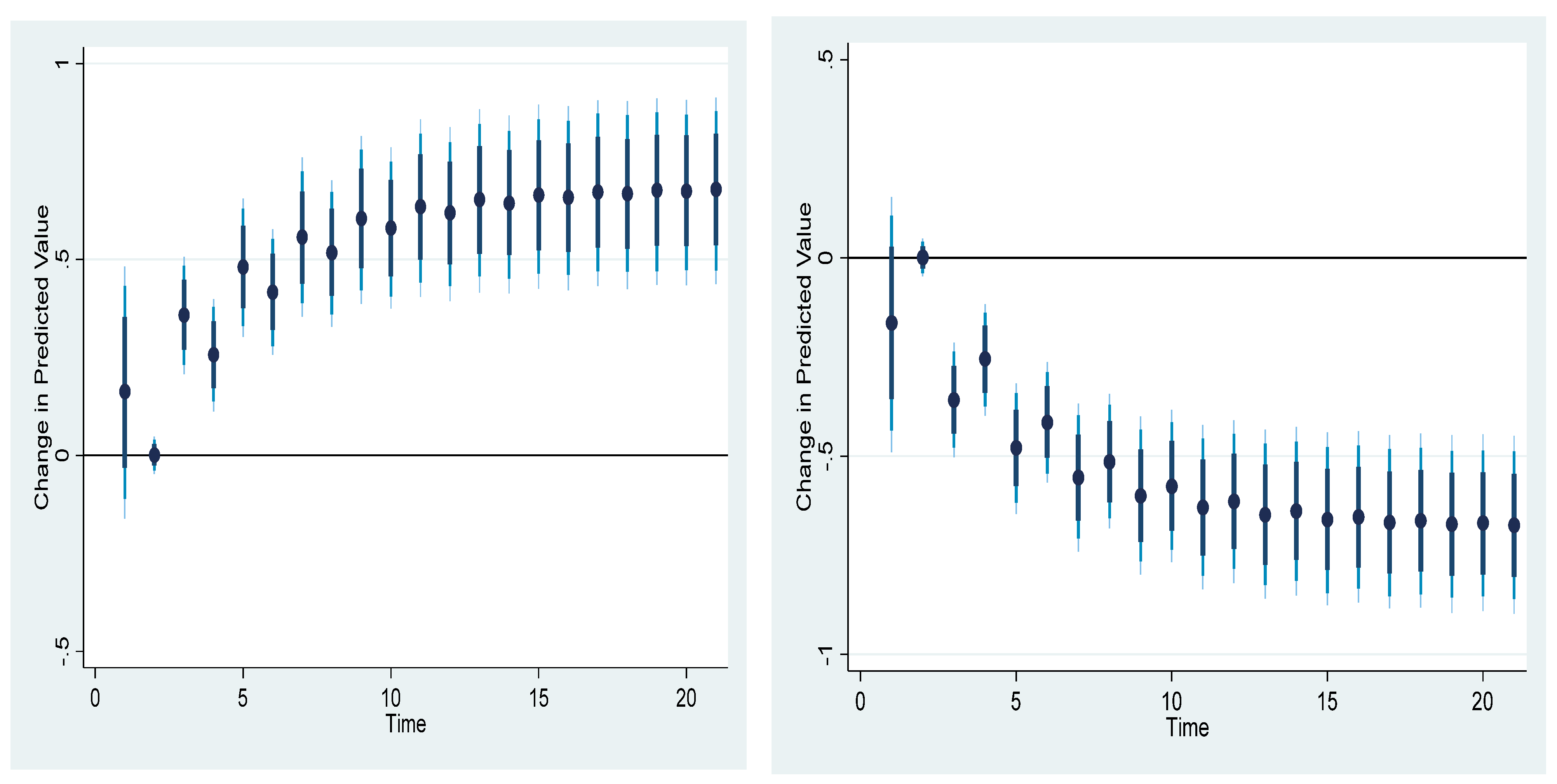
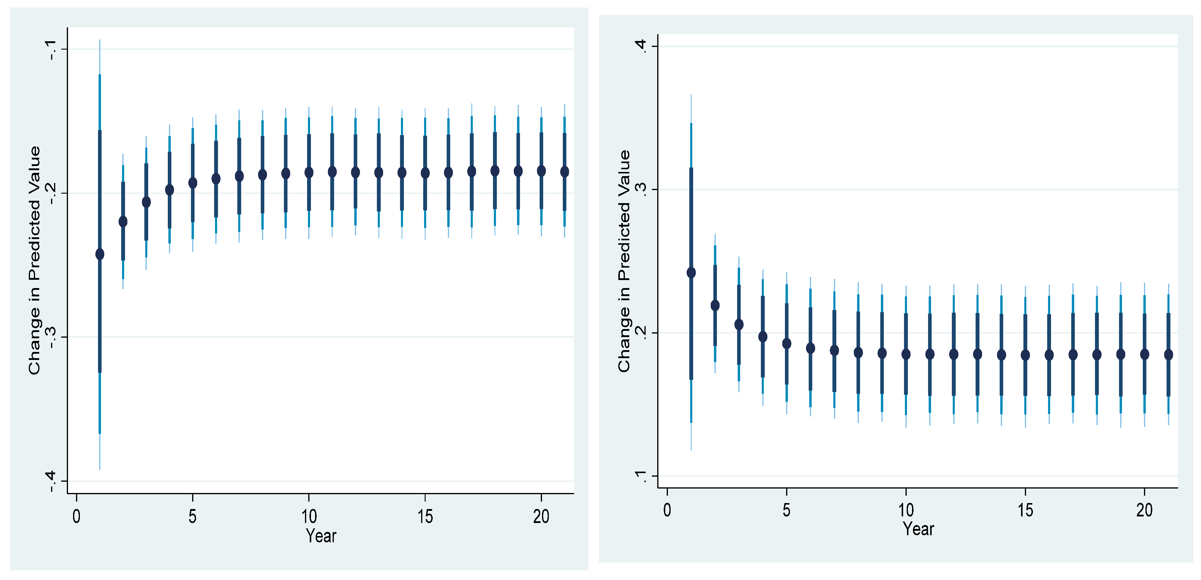
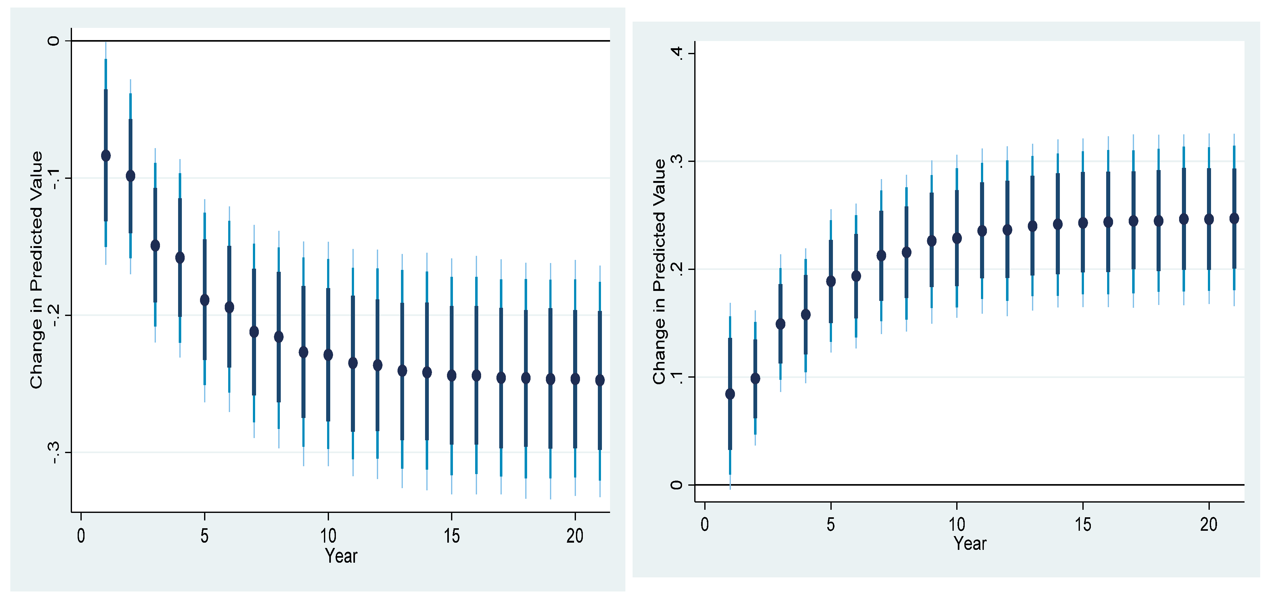
Figure 2 illustrates the impulse response plot between the export and the ecological footprint. The graph shows how changes in exports impact the ecological footprint in India. The anticipated value is shown by the dots in the figure, while the deep blue line represents the 75 percent confidence interval, and the light blue to lightest blue lines reflect the 90 percent and 95 percent confidence intervals, respectively. Figure 2 unveils that every 10% increase in exports is associated with a corresponding decrease in the ecological footprint of India. In contrast, a 10% decrease in exports corroborates to the corresponding increase in the ecological footprint of India. Figure 2 also uncovers that both the positive and negative shock of exports have almost the same impact on the ecological footprint of India. Figure 3 depicts the impulse response plot between the industry value added and the ecological footprint. This figure tells that every 10% increase in IVA deepens the ecological footprint of India, while every 10% decrease in IVA plummets the environmental dilapidation. Furthermore, the impulse response plot between the GDP and the ecological footprint, as shown in Figure 4, illustrates that every 10% increase in the GDP soars the environmental decrepitude, while every 10% decrease in the GDP contributes towards the environmental correction. Moreover, the impulse response plot between renewable energy consumption and the ecological footprint, as depicted in Figure 5, says that every 10% increase in renewable energy consumption contributes to the pathway of ecological footprint neutralization, while every 10% decrease in renewable energy consumption intensifies the ecological footprint of India.

4.5. Model Diagnostics and Robustness Test

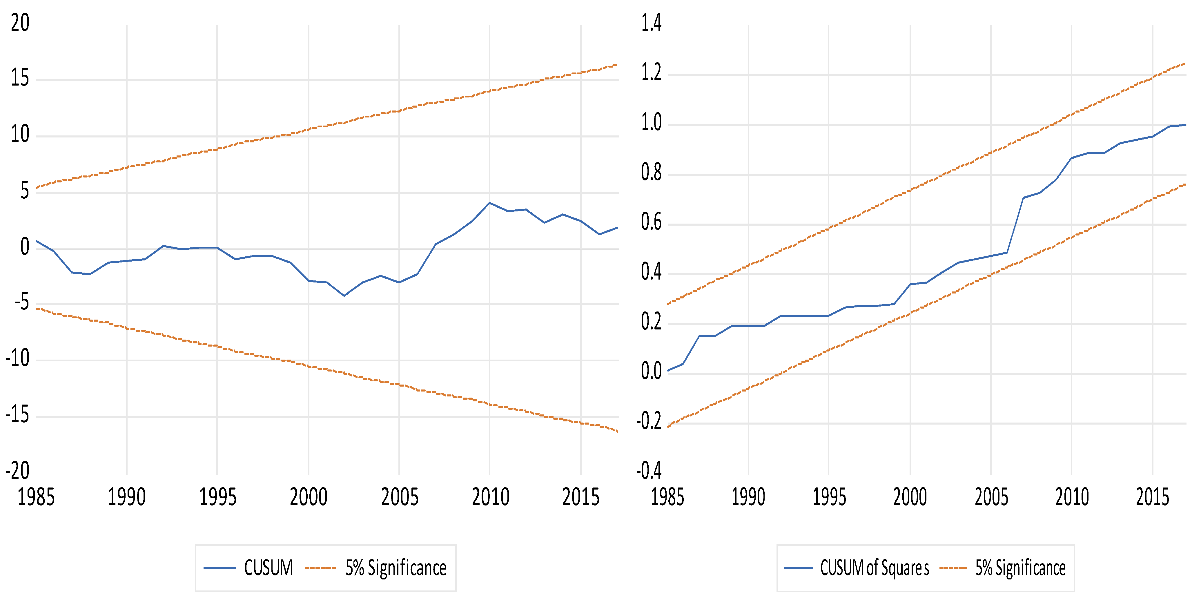
The credibility of our model and outcomes have been further verified through some post-diagnostic tests and by applying ARDL, FMOLS, and DOLS, respectively. The outcomes of the post-diagnostics tests, as shown in Table 7, unveils that our estimated model has passed the Jarque–Bera test of normality, Breusch–Godfrey serial correlation LM test, Breusch–Pagan–Godfrey test of heteroscedasticity, and the specification test. The outcomes of the stability test, as depicted in Figure 6, certify that the estimated D-ARDL model has passed the stability test, as the plots of both CUSUM and CUSUMQ are well within the 95% critical limit.
The essence of augmenting the ARDL, FMOLS, and CCR approaches is to cross-validate the outcomes of the D-ARDL estimations. The outcomes of the long-run coefficient estimates, as given in Table 8, seem to be consistent with the D-ARDL estimations, as given in Table 6. This further certifies the usability of the D-ARDL outcomes for further policy inferences.

4.6. Analysis of Causality

The pairwise causality analysis has also been done by augmenting the Breitung and Candelon [85] frequency domain causality test (Table 9). The results of this test have provided empirical evidence of (i) unidirectional causality from the GDP to the ecological footprint in long run, (ii) unidirectional causality from the industry value added to the ecological footprint in long run, and (iii) a short-run causality from renewable energy consumption to the ecological footprint. This could be because of the comparatively larger land requirement for setting up renewable energy plants, which possibly get compensated in long run through clean energy consumption in the economy.

5. Conclusions and Policy Recommendations

5.1. Conclusions

The main theme of this study is to empirically examine the influence of exports, the GDP, industry value added, and renewable energy consumption on the EF of India, during the period spanning from 1970–2017. For this purpose, the recently developed augmented ARDL (A-ARDL) bounds test, by McNown et al. [79], has been employed to explore the long-run co-integration among the variables. The dynamic ARDL (D-ARDL) simulations model has also been adopted to estimate the short- and long-run coefficient estimates of the EF determinants for India. The outcomes of the D-ARDL approach provide some fresh insights. This study not only confirms the existence of long-run dynamics among the core variables of this study but also confirms the EKC hypothesis for India. While export and renewable energy consumption seem to improve the environmental quality, industry value added seems to be accompanied by the corresponding obliteration of environmental well-being. Further, the association of industrialization with negative environmental externalities heightens the conflict between two seemingly ambitious goals of India, i.e., “Make in India” by achieving higher economic growth through enriching indigenous manufacturing, and “INDC” by reducing the targeted carbon emissions. In addition, the spectral causality test has also been used to predict the pairwise causality among the variables. The findings of this approach reveal unidirectional long-run causality from both the GDP and the industry value added to EF. However, the short-run causality from renewable energy consumption to the ecological footprint shows that renewable energy penetration may impact the ecological footprint in the short run.

5.2. Policy Recommendations

The results of this study can have implications for some significant policy decisions. As we found that renewable energy has a significant beneficial impact on the environmental conditions in India, policy emphasis is needed to prompt greater renewable energy use, from household consumption to the industry level. The use of renewable energy at the household level may be encouraged by raising environmental awareness among people, offering subsidies, and securing tax exemptions from the state and federal governments. However, at the industry level, the necessary funds, credit facilities, and tax incentives are needed to promote the use of clean energy sources at the industrial level. Conversely, the legislation of the Pigouvian tax can be applied to industries that utilize non-renewable energy more frequently. These policy measures can be beneficial in reducing the ecological footprint of industrialization as well.
According to our empirical results, India may be able to reduce its ecological footprint and achieve sustainable growth through the expansion of the export sector. The Indian government must develop long-term plans to increase the country’s trading basket in order to reap the benefits of exports. The government must consider the cost-effectiveness of producing exportable goods, the use of cutting-edge technology in the manufacturing process, the adoption of energy-efficient equipment, the reliable supply of raw materials, and the political stability of the nation when developing a long-term strategy for the green export sector. In this context, it is essential to increase the export mix of the nation’s knowledge-based products, which are typically less harmful to environmental quality. In 2021, India witnessed an 18.7% growth in exports from the services sector as compared to a 4.82% increase in merchandise exports in 2020. Although this could be an outcome of a two-year pandemic, India still needs to plan for similar growth trends in exports. The results of this study also indicate that India’s export basket possibly represents its comparative advantage in terms of its ecological footprint as well. In addition, more sustainable growth through exports can be possible if there is policy emphasis on improving the efficiency of production in this sector, reducing energy intensity, and reducing resource intensity through technology and innovation. Close monitoring, data collection, and political will are, however, needed to channel trade instruments, such as subsidies, to boost the export sector and ensure that the resource intensity of exports is not just maintained but reduced through strong efficiency norms and environmental standards of production that can additionally make Indian exports more attractive to the world market.
Given that the strategies proposed in this study only took a few aggregated economic elements into account, further studies can consider demographic factors to increase the robustness of the policy formation. However, the policies outlined in this study can still serve as a baseline report that can be developed further. Future research on this topic can take into account the geographical aspects of demographic disparities, as this can provide a number of fresh perspectives on the pattern of changes in the ecological footprint. Therefore, more research may be done by considering a larger economic area or group of nations, as well as other crucial factors such as export diversification, R&D spending, green innovation, etc.

Author Contributions

Conceptualization, S.R. and B.N.; methodology, S.R.; software, S.R.; validation, S.R., B.N. and M.E.H.; formal analysis, B.N.; investigation, M.E.H.; resources, S.R.; data curation, B.N. and M.E.H.; writing—original draft preparation, S.R., B.N. and M.E.H.; writing—review and editing, S.R., B.N. and M.E.H.; visualization, M.E.H.; supervision, B.N.; project administration, B.N.; funding acquisition, S.R. and B.N. All authors have read and agreed to the published version of the manuscript.

Funding

This research received no external funding.

Institutional Review Board Statement

Not applicable.

Informed Consent Statement

Not applicable.

Data Availability Statement

Data can be freely available from https://www.footprintnetwork.org/ and https://data.worldbank.org/ (accessed on 10 September 2022) and https://www.bp.com/en/global/corporate/energy-economics/statistical-review-of-world-energy.html (accessed on 10 September 2022).

Conflicts of Interest

The authors declare no conflict of interest.

References

  1. Caglar, A.E. Can Nuclear Energy Technology Budgets Pave the Way for a Transition toward Low-Carbon Economy: Insights from the United Kingdom. Sustain. Dev. 2022. [Google Scholar] [CrossRef]
  2. Caglar, A.E.; Ulug, M. The Role of Government Spending on Energy Efficiency R&D Budgets in the Green Transformation Process: Insight from the Top-Five Countries. Environ. Sci. Pollut. Res. 2022, 29, 76472–76484. [Google Scholar]
  3. Caglar, A.E.; Mert, M. Carbon Hysteresis Hypothesis as a New Approach to Emission Behavior: A Case of Top Five Emitters. Gondwana Res. 2022, 109, 171–182. [Google Scholar] [CrossRef]
  4. Global Footprint Network Google Scholar. Available online: https://www.footprintnetwork.org/content/uploads/2022/09/BAK_Economics_Sustainability_22092022.pdf (accessed on 19 October 2022).
  5. Mitić, P.; Munitlak Ivanović, O.; Zdravković, A. A Cointegration Analysis of Real GDP and CO2 Emissions in Transitional Countries. Sustainability 2017, 9, 568. [Google Scholar] [CrossRef] [Green Version]
  6. Gong, B.; Zheng, X.; Guo, Q.; Ordieres-Meré, J. Discovering the Patterns of Energy Consumption, GDP, and CO2 Emissions in China Using the Cluster Method. Energy 2019, 166, 1149–1167. [Google Scholar] [CrossRef]
  7. MoC Google Scholar. Available online: https://commerce.gov.in/wp-content/uploads/2020/02/MOC_636434269763910839_international_tpp_DFTP.pdf (accessed on 19 October 2022).
  8. Ram, R. Exports and Economic Growth in Developing Countries: Evidence from Time-Series and Cross-Section Data. Econ. Dev. Cult. Chang. 1987, 36, 51–72. [Google Scholar] [CrossRef]
  9. Ekanayake, E.M. Exports and Economic Growth in Asian Developing Countries: Cointegration and Error-Correction Models. J. Econ. Dev. 1999, 24, 43–56. [Google Scholar]
  10. MoRE Google Scholar. Available online: https://mnre.gov.in/img/documents/uploads/file_f-1618564141288.pdf (accessed on 19 October 2022).
  11. Apergis, N.; Can, M.; Gozgor, G.; Lau, C.K.M. Effects of Export Concentration on CO2 Emissions in Developed Countries: An Empirical Analysis. Environ. Sci. Pollut. Res. 2018, 25, 14106–14116. [Google Scholar] [CrossRef] [Green Version]
  12. Haug, A.A.; Ucal, M. The Role of Trade and FDI for CO2 Emissions in Turkey: Nonlinear Relationships. Energy Econ. 2019, 81, 297–307. [Google Scholar] [CrossRef]
  13. Rahman, M.M.; Nepal, R.; Alam, K. Impacts of Human Capital, Exports, Economic Growth and Energy Consumption on CO2 Emissions of a Cross-Sectionally Dependent Panel: Evidence from the Newly Industrialized Countries (NICs). Environ. Sci. Policy 2021, 121, 24–36. [Google Scholar] [CrossRef]
  14. Gozgor, G.; Can, M. Does Export Product Quality Matter for CO2 Emissions? Evidence from China. Environ. Sci. Pollut. Res. 2017, 24, 2866–2875. [Google Scholar] [CrossRef] [PubMed]
  15. Hossain, M.E.; Rej, S.; Saha, S.M.; Onwe, J.C.; Nwulu, N.; Bekun, F.V.; Taha, A. Can Energy Efficiency Help in Achieving Carbon-Neutrality Pledges? A Developing Country Perspective Using Dynamic ARDL Simulations. Sustainability 2022, 14, 7537. [Google Scholar] [CrossRef]
  16. Li, K.; Lin, B. Impacts of Urbanization and Industrialization on Energy Consumption/CO2 Emissions: Does the Level of Development Matter? Renew. Sustain. Energy Rev. 2015, 52, 1107–1122. [Google Scholar] [CrossRef]
  17. Zaidi, S.A.H.; Hou, F.; Mirza, F.M. The Role of Renewable and Non-Renewable Energy Consumption in CO2 Emissions: A Disaggregate Analysis of Pakistan. Environ. Sci. Pollut. Res. 2018, 25, 31616–31629. [Google Scholar] [CrossRef] [PubMed]
  18. Bulut, U. The Impacts of Non-Renewable and Renewable Energy on CO2 Emissions in Turkey. Environ. Sci. Pollut. Res. 2017, 24, 15416–15426. [Google Scholar] [CrossRef]
  19. Chen, Y.; Wang, Z.; Zhong, Z. CO2 Emissions, Economic Growth, Renewable and Non-Renewable Energy Production and Foreign Trade in China. Renew. Energy 2019, 131, 208–216. [Google Scholar] [CrossRef]
  20. Long, X.; Naminse, E.Y.; Du, J.; Zhuang, J. Nonrenewable Energy, Renewable Energy, Carbon Dioxide Emissions and Economic Growth in China from 1952 to 2012. Renew. Sustain. Energy Rev. 2015, 52, 680–688. [Google Scholar] [CrossRef]
  21. Sharma, R.; Sinha, A.; Kautish, P. Does Renewable Energy Consumption Reduce Ecological Footprint? Evidence from Eight Developing Countries of Asia. J. Clean. Prod. 2021, 285, 124867. [Google Scholar] [CrossRef]
  22. Inglesi-Lotz, R.; Dogan, E. The Role of Renewable versus Non-Renewable Energy to the Level of CO2 Emissions a Panel Analysis of Sub-Saharan Africa’s Big 10 Electricity Generators. Renew. Energy 2018, 123, 36–43. [Google Scholar] [CrossRef] [Green Version]
  23. Dogan, E.; Seker, F. Determinants of CO2 Emissions in the European Union: The Role of Renewable and Non-Renewable Energy. Renew. Energy 2016, 94, 429–439. [Google Scholar] [CrossRef]
  24. Wackernagel, M.; Rees, W. Our Ecological Footprint: Reducing Human Impact on the Earth; New Society Publishers: Gabriola, Canada, 1998; Volume 9. [Google Scholar]
  25. Destek, M.A.; Sinha, A. Renewable, Non-Renewable Energy Consumption, Economic Growth, Trade Openness and Ecological Footprint: Evidence from Organisation for Economic Co-Operation and Development Countries. J. Clean. Prod. 2020, 242, 118537. [Google Scholar] [CrossRef]
  26. Sharif, A.; Raza, S.A.; Ozturk, I.; Afshan, S. The Dynamic Relationship of Renewable and Nonrenewable Energy Consumption with Carbon Emission: A Global Study with the Application of Heterogeneous Panel Estimations. Renew. Energy 2019, 133, 685–691. [Google Scholar] [CrossRef]
  27. Bello, M.O.; Solarin, S.A.; Yen, Y.Y. The Impact of Electricity Consumption on CO2 Emission, Carbon Footprint, Water Footprint and Ecological Footprint: The Role of Hydropower in an Emerging Economy. J. Environ. Manag. 2018, 219, 218–230. [Google Scholar] [CrossRef] [PubMed]
  28. Ben Jebli, M.; Ben Youssef, S.; Apergis, N. The Dynamic Linkage between Renewable Energy, Tourism, CO2 Emissions, Economic Growth, Foreign Direct Investment, and Trade. Lat. Am. Econ. Rev. 2019, 28, 1–19. [Google Scholar] [CrossRef] [Green Version]
  29. Sharif, A.; Baris-Tuzemen, O.; Uzuner, G.; Ozturk, I.; Sinha, A. Revisiting the Role of Renewable and Non-Renewable Energy Consumption on Turkey’s Ecological Footprint: Evidence from Quantile ARDL Approach. Sustain. Cities Soc. 2020, 57, 102138. [Google Scholar] [CrossRef]
  30. Christoforidis, T.; Katrakilidis, C. Does Foreign Direct Investment Matter for Environmental Degradation? Empirical Evidence from Central–Eastern European Countries. J. Knowl. Econ. 2021, 1–30. [Google Scholar] [CrossRef]
  31. Xue, L.; Haseeb, M.; Mahmood, H.; Alkhateeb, T.T.Y.; Murshed, M. Renewable Energy Use and Ecological Footprints Mitigation: Evidence from Selected South Asian Economies. Sustainability 2021, 13, 1613. [Google Scholar] [CrossRef]
  32. Dogan, E.; Shah, S.F. Analyzing the Role of Renewable Energy and Energy Intensity in the Ecological Footprint of the United Arab Emirates. Sustainability 2022, 14, 227. [Google Scholar] [CrossRef]
  33. Kim, S. The Effects of Foreign Direct Investment, Economic Growth, Industrial Structure, Renewable and Nuclear Energy, and Urbanization on Korean Greenhouse Gas Emissions. Sustainability 2020, 12, 1625. [Google Scholar] [CrossRef] [Green Version]
  34. Akadiri, S.S.; Adebayo, T.S. Asymmetric Nexus among Financial Globalization, Non-Renewable Energy, Renewable Energy Use, Economic Growth, and Carbon Emissions: Impact on Environmental Sustainability Targets in India. Environ. Sci. Pollut. Res. 2021, 29, 16311–16323. [Google Scholar] [CrossRef]
  35. Rej, S.; Nag, B. Investigating the Role of Capital Formation to Achieve Carbon Neutrality in India. Environ. Sci. Pollut. Res. 2022, 29, 60472–60490. [Google Scholar] [CrossRef] [PubMed]
  36. Sadorsky, P. Energy Consumption, Output and Trade in South America. Energy Econ. 2012, 34, 476–488. [Google Scholar] [CrossRef]
  37. Liu, H.; Kim, H.; Choe, J. Export Diversification, CO2 Emissions and EKC: Panel Data Analysis of 125 Countries. Asia-Pac. J. Reg. Sci. 2019, 3, 361–393. [Google Scholar] [CrossRef]
  38. Gozgor, G.; Can, M. Export Product Diversification and the Environmental Kuznets Curve: Evidence from Turkey. Environ. Sci. Pollut. Res. 2016, 23, 21594–21603. [Google Scholar] [CrossRef] [Green Version]
  39. Mania, E. Export Diversification and CO2 Emissions: An Augmented Environmental Kuznets Curve. J. Int. Dev. 2020, 32, 168–185. [Google Scholar] [CrossRef]
  40. Sharma, R.; Sinha, A.; Kautish, P. Examining the Nexus between Export Diversification and Environmental Pollution: Evidence from BRICS Nations. Environ. Sci. Pollut. Res. 2021, 28, 61732–61747. [Google Scholar] [CrossRef] [PubMed]
  41. Zafar, M.W.; Saleem, M.M.; Destek, M.A.; Caglar, A.E. The Dynamic Linkage between Remittances, Export Diversification, Education, Renewable Energy Consumption, Economic Growth, and CO2 Emissions in Top Remittance-Receiving Countries. Sustain. Dev. 2022, 30, 165–175. [Google Scholar] [CrossRef]
  42. Islam, M.; Hossain, M.; Khan, M.; Rana, M.; Ema, N.S.; Bekun, F.V. Heading towards Sustainable Environment: Exploring the Dynamic Linkage among Selected Macroeconomic Variables and Ecological Footprint Using a Novel Dynamic ARDL Simulations Approach. Environ. Sci. Pollut. Res. 2022, 29, 22260–22279. [Google Scholar] [CrossRef]
  43. Charfeddine, L. The Impact of Energy Consumption and Economic Development on Ecological Footprint and CO2 Emissions: Evidence from a Markov Switching Equilibrium Correction Model. Energy Econ. 2017, 65, 355–374. [Google Scholar] [CrossRef]
  44. Alola, A.A.; Bekun, F.V.; Sarkodie, S.A. Dynamic Impact of Trade Policy, Economic Growth, Fertility Rate, Renewable and Non-Renewable Energy Consumption on Ecological Footprint in Europe. Sci. Total Environ. 2019, 685, 702–709. [Google Scholar] [CrossRef]
  45. Hu, H.; Xie, N.; Fang, D.; Zhang, X. The Role of Renewable Energy Consumption and Commercial Services Trade in Carbon Dioxide Reduction: Evidence from 25 Developing Countries. Appl. Energy 2018, 211, 1229–1244. [Google Scholar] [CrossRef]
  46. Dogan, B.; Madaleno, M.; Tiwari, A.K.; Hammoudeh, S. Impacts of Export Quality on Environmental Degradation: Does Income Matter? Environ. Sci. Pollut. Res. 2020, 27, 13735–13772. [Google Scholar] [CrossRef]
  47. Rahman, M.M. Do Population Density, Economic Growth, Energy Use and Exports Adversely Affect Environmental Quality in Asian Populous Countries? Renew. Sustain. Energy Rev. 2017, 77, 506–514. [Google Scholar] [CrossRef]
  48. Hausmann, R.; Hwang, J.; Rodrik, D. What You Export Matters. J. Econ. Growth 2007, 12, 1–25. [Google Scholar] [CrossRef]
  49. Harding, T.; Javorcik, B.S. Foreign Direct Investment and Export Upgrading. Rev. Econ. Stat. 2012, 94, 964–980. [Google Scholar] [CrossRef]
  50. Alam, J. Impact of Agriculture, Industry and Service Sector’s Value Added in the GDP on CO2 Emissions of Selected South Asian Countries. World Rev. Bus. Res. 2015, 5, 39–59. [Google Scholar]
  51. Huan, Y.; Hassan, M.S.; Tahir, M.N.; Mahmood, H.; Al-Darwesh, H.R.I. The Role of Energy Use in Testing N–Shaped Relation between Industrial Development and Environmental Quality for Chinese Economy. Energy Strategy Rev. 2022, 43, 100905. [Google Scholar] [CrossRef]
  52. Liu, X.; Bae, J. Urbanization and Industrialization Impact of CO2 Emissions in China. J. Clean. Prod. 2018, 172, 178–186. [Google Scholar] [CrossRef]
  53. Liu, Y.; Hao, Y. The Dynamic Links between CO2 Emissions, Energy Consumption and Economic Development in the Countries along “the Belt and Road". Sci. Total Environ. 2018, 645, 674–683. [Google Scholar] [CrossRef]
  54. Dong, F.; Wang, Y.; Su, B.; Hua, Y.; Zhang, Y. The Process of Peak CO2 Emissions in Developed Economies: A Perspective of Industrialization and Urbanization. Resour. Conserv. Recycl. 2019, 141, 61–75. [Google Scholar] [CrossRef]
  55. Ullah, S.; Ozturk, I.; Usman, A.; Majeed, M.T.; Akhtar, P. On the Asymmetric Effects of Premature Deindustrialization on CO2 Emissions: Evidence from Pakistan. Environ. Sci. Pollut. Res. 2020, 27, 13692–13702. [Google Scholar] [CrossRef]
  56. Mentel, U.; Wolanin, E.; Eshov, M.; Salahodjaev, R. Industrialization and CO2 Emissions in Sub-Saharan Africa: The Mitigating Role of Renewable Electricity. Energies 2022, 15, 946. [Google Scholar] [CrossRef]
  57. Appiah, M.; Li, F.; Korankye, B. Modeling the Linkages among CO2 Emission, Energy Consumption, and Industrialization in Sub-Saharan African (SSA) Countries. Environ. Sci. Pollut. Res. 2021, 28, 38506–38521. [Google Scholar] [CrossRef]
  58. Yang, X.; Khan, I. Dynamics among Economic Growth, Urbanization, and Environmental Sustainability in IEA Countries: The Role of Industry Value-Added. Environ. Sci. Pollut. Res. 2022, 29, 4116–4127. [Google Scholar] [CrossRef]
  59. Abbasi, K.R.; Hussain, K.; Redulescu, M.; Ozturk, I. Does Natural Resources Depletion and Economic Growth Achieve the Carbon Neutrality Target of the UK? A Way Forward towards Sustainable Development. Resour. Policy 2021, 74, 102341. [Google Scholar] [CrossRef]
  60. Khan, R. Beta Decoupling Relationship between CO2 Emissions by GDP, Energy Consumption, Electricity Production, Value-Added Industries, and Population in China. PLoS ONE 2021, 16, e0249444. [Google Scholar] [CrossRef]
  61. Shahbaz, M.; Khraief, N.; Uddin, G.S.; Ozturk, I. Environmental Kuznets Curve in an Open Economy: A Bounds Testing and Causality Analysis for Tunisia. Renew. Sustain. Energy Rev. 2014, 34, 325–336. [Google Scholar] [CrossRef] [Green Version]
  62. Furuoka, F. The CO2 Emissions–Development Nexus Revisited. Renew. Sustain. Energy Rev. 2015, 51, 1256–1275. [Google Scholar] [CrossRef]
  63. Magazzino, C.; Porrini, D.; Fusco, G.; Schneider, N. Investigating the Link among ICT, Electricity Consumption, Air Pollution, and Economic Growth in EU Countries. Energy Sour. Part B Econ. Plan. Policy 2021, 16, 976–998. [Google Scholar]
  64. Gyamfi, B.A.; Adedoyin, F.F.; Bein, M.A.; Bekun, F.V. Environmental Implications of N-Shaped Environmental Kuznets Curve for E7 Countries. Environ. Sci. Pollut. Res. 2021, 28, 33072–33082. [Google Scholar] [CrossRef]
  65. Ozcan, B.; Tzeremes, P.G.; Tzeremes, N.G. Energy Consumption, Economic Growth and Environmental Degradation in OECD Countries. Econ. Model. 2020, 84, 203–213. [Google Scholar] [CrossRef]
  66. Shahbaz, M.; Haouas, I.; Van Hoang, T.H. Economic Growth and Environmental Degradation in Vietnam: Is the Environmental Kuznets Curve a Complete Picture? Emerg. Mark. Rev. 2019, 38, 197–218. [Google Scholar] [CrossRef]
  67. Naseem, S.; Mohsin, M.; Zia-UR-Rehman, M.; Baig, S.A.; Sarfraz, M. The Influence of Energy Consumption and Economic Growth on Environmental Degradation in BRICS Countries: An Application of the ARDL Model and Decoupling Index. Environ. Sci. Pollut. Res. 2022, 29, 13042–13055. [Google Scholar] [CrossRef]
  68. Rahman, H.U.; Zaman, U.; Górecki, J. The Role of Energy Consumption, Economic Growth and Globalization in Environmental Degradation: Empirical Evidence from the Brics Region. Sustainability 2021, 13, 1924. [Google Scholar] [CrossRef]
  69. Danish, H.S.; Baloch, M.A.; Mahmood, N.; Zhang, J.W. Linking Economic Growth and Ecological Footprint through Human Capital and Biocapacity. Sustain. Cities Soc. 2019, 47, 101516. [Google Scholar] [CrossRef]
  70. Ahmad, M.; Jiang, P.; Majeed, A.; Umar, M.; Khan, Z.; Muhammad, S. The Dynamic Impact of Natural Resources, Technological Innovations and Economic Growth on Ecological Footprint: An Advanced Panel Data Estimation. Resour. Policy 2020, 69, 101817. [Google Scholar] [CrossRef]
  71. Ahmed, Z.; Asghar, M.M.; Malik, M.N.; Nawaz, K. Moving towards a Sustainable Environment: The Dynamic Linkage between Natural Resources, Human Capital, Urbanization, Economic Growth, and Ecological Footprint in China. Resour. Policy 2020, 67, 101677. [Google Scholar] [CrossRef]
  72. Galli, A.; Kitzes, J.; Niccolucci, V.; Wackernagel, M.; Wada, Y.; Marchettini, N. Assessing the Global Environmental Consequences of Economic Growth through the Ecological Footprint: A Focus on China and India. Ecol. Indic. 2012, 17, 99–107. [Google Scholar] [CrossRef]
  73. Ahmed, Z.; Wang, Z. Investigating the Impact of Human Capital on the Ecological Footprint in India: An Empirical Analysis. Environ. Sci. Pollut. Res. 2019, 26, 26782–26796. [Google Scholar] [CrossRef]
  74. Murshed, M.; Nurmakhanova, M.; Al-Tal, R.; Mahmood, H.; Elheddad, M.; Ahmed, R. Can Intra-Regional Trade, Renewable Energy Use, Foreign Direct Investments, and Economic Growth Mitigate Ecological Footprints in South Asia? Energy Sour. Part B Econ. Plan. Policy 2022, 1–26. [Google Scholar] [CrossRef]
  75. Adebayo, T.S.; Akadiri, S.S.; Altuntaş, M.; Awosusi, A.A. Environmental Effects of Structural Change, Hydro and Coal Energy Consumption on Ecological Footprint in India: Insights from the Novel Dynamic ARDL Simulation. Environ. Dev. Sustain. 2022, 1–24. [Google Scholar] [CrossRef]
  76. Engle, R.F.; Granger, C.W. Co-Integration and Error Correction: Representation, Estimation, and Testing. Econom. J. Econom. Soc. 1987, 55, 251–276. [Google Scholar] [CrossRef]
  77. Johansen, S.; Juselius, K. Maximum Likelihood Estimation and Inference on Cointegration—With Appucations to the Demand for Money. Oxf. Bull. Econ. Stat. 1990, 52, 169–210. [Google Scholar] [CrossRef]
  78. Pesaran, M.H.; Shin, Y.; Smith, R.J. Bounds Testing Approaches to the Analysis of Level Relationships. J. Appl. Econom. 2001, 16, 289–326. [Google Scholar] [CrossRef]
  79. McNown, R.; Sam, C.Y.; Goh, S.K. Bootstrapping the Autoregressive Distributed Lag Test for Cointegration. Appl. Econ. 2018, 50, 1509–1521. [Google Scholar] [CrossRef]
  80. Sam, C.Y.; McNown, R.; Goh, S.K. An Augmented Autoregressive Distributed Lag Bounds Test for Cointegration. Econ. Model. 2019, 80, 130–141. [Google Scholar] [CrossRef]
  81. Narayan, P.K. The Saving and Investment Nexus for China: Evidence from Cointegration Tests. Appl. Econ. 2005, 37, 1979–1990. [Google Scholar] [CrossRef]
  82. Jordan, S.; Philips, A.Q. Cointegration Testing and Dynamic Simulations of Autoregressive Distributed Lag Models. Stata J. 2018, 18, 902–923. [Google Scholar] [CrossRef] [Green Version]
  83. Hossain, M.E.; Islam, M.S.; Bandyopadhyay, A.; Awan, A.; Hossain, M.R.; Rej, S. Mexico at the Crossroads of Natural Resource Dependence and COP26 Pledge: Does Technological Innovation Help? Resour. Policy 2022, 77, 102710. [Google Scholar] [CrossRef]
  84. Hossain, M.; Islam, M.; Sujan, M.; Khan, H.; Tuhin, M.; Bekun, F.V. Towards a Clean Production by Exploring the Nexus between Agricultural Ecosystem and Environmental Degradation Using Novel Dynamic ARDL Simulations Approach. Environ. Sci. Pollut. Res. 2022, 29, 53768–53784. [Google Scholar] [CrossRef]
  85. Breitung, J.; Candelon, B. Testing for Short-and Long-Run Causality: A Frequency-Domain Approach. J. Econom. 2006, 132, 363–378. [Google Scholar] [CrossRef]
  86. Narayan, P.K.; Narayan, S. Carbon Dioxide Emissions and Economic Growth: Panel Data Evidence from Developing Countries. Energy Policy 2010, 38, 661–666. [Google Scholar] [CrossRef]
  87. Rej, S.; Bandyopadhyay, A.; Das, N.; Hossain, M.; Islam, M.; Bera, P.; Yeediballi, T. The Asymmetric Influence of Environmental-Related Technological Innovation on Climate Change Mitigation: What Role Do FDI and Renewable Energy Play? Environ. Sci. Pollut. Res. 2022, 1–16. [Google Scholar] [CrossRef]
  88. Kanjilal, K.; Ghosh, S. Environmental Kuznet’s Curve for India: Evidence from Tests for Cointegration with Unknown Structuralbreaks. Energy Policy 2013, 56, 509–515. [Google Scholar] [CrossRef]
  89. Jayanthakumaran, K.; Verma, R.; Liu, Y. CO2 Emissions, Energy Consumption, Trade and Income: A Comparative Analysis of China and India. Energy Policy 2012, 42, 450–460. [Google Scholar] [CrossRef]
  90. Bandyopadhyay, A.; Rej, S. Can Nuclear Energy Fuel an Environmentally Sustainable Economic Growth? Revisiting the EKC Hypothesis for India. Environ. Sci. Pollut. Res. 2021, 28, 63065–63086. [Google Scholar] [CrossRef]
  91. Rej, S.; Bandyopadhyay, A.; Mahmood, H.; Murshed, M.; Mahmud, S. The Role of Liquefied Petroleum Gas in Decarbonizing India: Fresh Evidence from Wavelet–Partial Wavelet Coherence Approach. Environ. Sci. Pollut. Res. 2022, 29, 35862–35883. [Google Scholar] [CrossRef]
  92. Bandyopadhyay, A.; Rej, S.; Abbasi, K.R.; Awan, A. Nexus between Tourism, Hydropower, and CO2 Emissions in India: Fresh Insights from ARDL and Cumulative Fourier Frequency Domain Causality. Environ. Dev. Sustain. 2022, 1–25. [Google Scholar] [CrossRef]
  93. Rej, S.; Bandyopadhyay, A.; Murshed, M.; Mahmood, H.; Razzaq, A. Pathways to Decarbonization in India: The Role of Environmentally Friendly Tourism Development. Environ. Sci. Pollut. Res. 2022, 29, 50281–50302. [Google Scholar] [CrossRef]
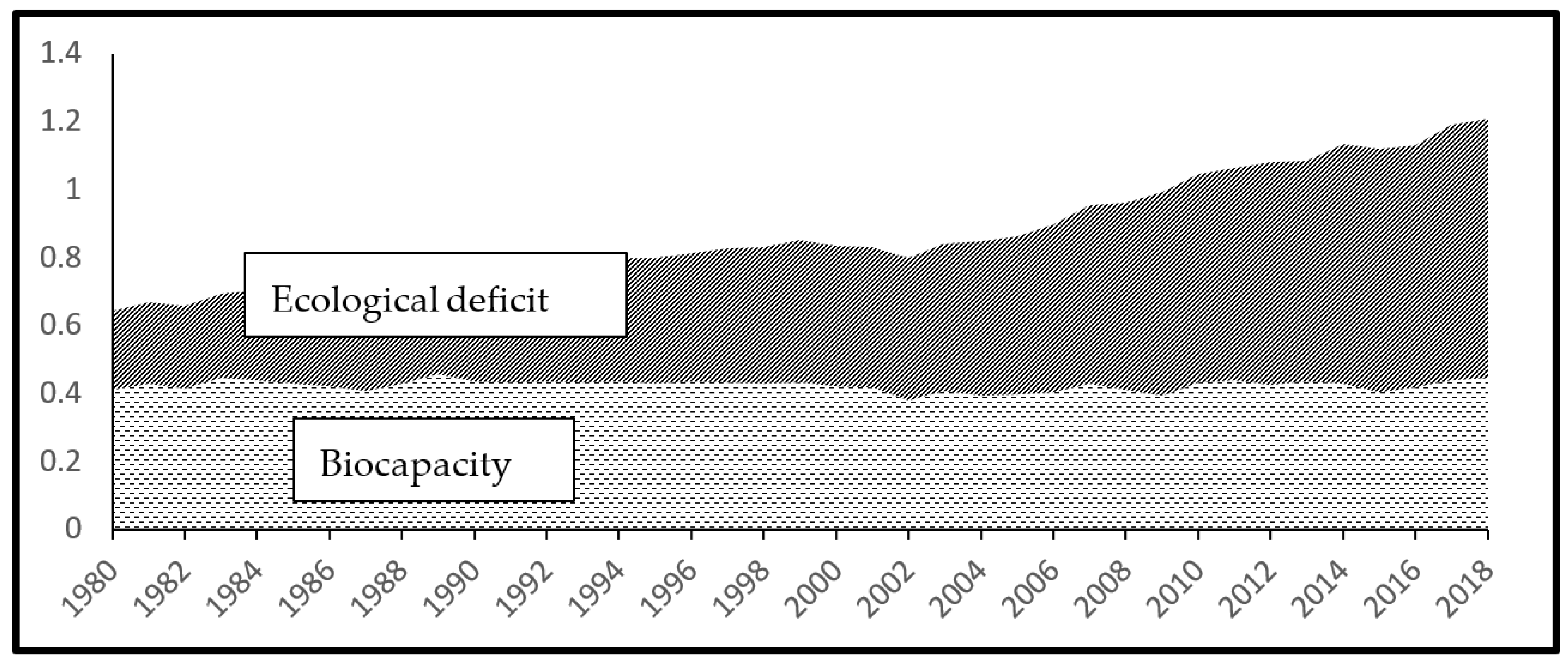
Figure 1. Per capita biocapacity and ecological deficit of the Indian economy from 1980–2018. Data source: Global Footprint Network, https://www.footprintnetwork.org/ (accessed on 10 September 2022).
Sustainability 14 15494 g001
Figure 2. The above figure signifies a 10% increase or decrease in export and their effect on the ecological footprint in India. Note: Years are used as the unit of time in the figure’s horizontal axis.
Sustainability 14 15494 g002
Figure 3. The above figure signifies a 10% increase or decrease in industry value added and their effect on the ecological footprint in India. Note: Years are used as the unit of time in the figure’s horizontal axis.
Sustainability 14 15494 g003
Figure 4. The above figure signifies a 10% increase or decrease in GDP and their effect on the ecological footprint in India.
Sustainability 14 15494 g004
Figure 5. The above figure signifies a 10% increase or decrease in renewable energy consumption and their effect on the ecological footprint in India.
Sustainability 14 15494 g005
Figure 6. The plot of CUSUM and CUSUM of square test.
Sustainability 14 15494 g006
Table 1. Variables Specification.
VariableDefinitionSource
EFEcological Footprint (global hectares/capita)Global Footprint Network
GDPEconomic growth (real GDP per capita constant 2015 US$)WDI
EXPExport of goods and services (% of GDP)WDI
IVAIndustry (including construction), value added (% of GDP)WDI
RECRenewable energy consumption (tonnes of oil equivalent/capita)BP Statistical Review of World Energy
Table 2. Descriptive statistics.
lnEFlnGDPlnEXPlnIVAlnREC
Mean−0.226.562.293.27−3.97
Median−0.236.442.283.29−4.05
Maximum0.187.593.233.44−3.24
Minimum−0.475.941.293.07−4.39
Std. Dev.0.190.510.590.090.31
Skewness0.530.490.13−0.590.85
Kurtosis2.161.971.683.262.69
Jarque-Bera3.674.053.613.012.78
Probability0.160.130.170.220.48
Observations4848484848
Correlation
lnEFlnGDPlnEXPlnIVAlnREC
lnEF1.00
lnGDP0.991.00
lnEXP0.930.951.00
lnIVA0.690.710.811.00
lnREC−0.910.890.840.621.00
Table 3. Unit Root test.
VariableFormADF (t-Statistics)PP (t-Statistics)Order of Integration
InterceptTrend + InterceptInterceptTrend + Intercept
lnEFLevel1.33
(0.998)
−2.13
(0.519)
1.71
(0.999)
−1.95
(0.612)
I(1)
First Difference−8.43 ***
(0.000)
−9.22 ***
(0.000)
−8.28 ***
(0.000)
−9.17 ***
(0.000)
lnGDPLevel4.19
(1.000)
−1.64
(0.761)
5.16
(1.000)
−1.87
(0.652)
I(1)
First Difference−5.69 ***
(0.000)
−8.25 ***
(0.000)
−5.75 ***
(0.000)
−11.94 ***
(0.000)
lnEXPLevel−1.25
(0.643)
−2.26
(0.448)
−1.23
(0.654)
−1.69
(0.738)
I(1)
First Difference−3.19 **
(0.027)
−3.27 **
(0.044)
−6.48 ***
(0.001)
−6.57 ***
(0.000)
lnIVALevel−2.25
(0.194)
−1.59
(0.779)
−2.38
(0.152)
−1.17
(0.905)
I(1)
First Difference−3.23 **
(0.025)
−3.66 **
(0.036)
−6.93 ***
(0.000)
−7.39 ***
(0.000)
lnRECLevel−0.04
(0.949)
−1.45
(0.832)
−0.04
(0.949)
−1.56
(0.792)
I(1)
First Difference−6.27 ***
(0.000)
−6.34 ***
(0.000)
−6.27 ***
(0.000)
−6.34 ***
(0.000)
Note: In parentheses, the probability value is given. ***, ** and * denotes a 1%, 5% and 10% level of significance.
Table 4. Zivot and Andrews structural break test.
VariableLevelFirst Difference
t-StatisticsTime Breakt-StatisticsTime Break
lnEF−4.31 ***2000−9.86 **2006
lnGDP−1.312003−5.11 **1991
lnEXP−2.962002−4.87 ***1987
lnLIVA−3.04 **2006−4.93 ***2002
lnREC−3.652000−4.37 **2004
Note: *** denotes a 1% level of significance, ** denotes a 5% level of significance, and * denotes a 10% level of significance.
Table 5. Augmented-ARDL Cointegration Results.
DV|LDVLag-LengthTest StatisticsResults
LEFt|LGDP, LEXP, LIVA, LREC, Dummy4, 1, 4, 1, 3, 2FOverall: 6.95 ***Cointegrated
tDV: −4.11 *
FIDV: 8.30 ***
Table CVs1%5%10%For k = 5
TestsI(0)I(1)I(0)I(1)I(0)I(1)Sources
FOverall3.414.682.623.792.263.35Narayan (2005)
tDV−3.43−4.79−2.86−4.19−2.57−3.86Pesaran et al. [79]
FLDV3.055.022.243.901.863.39Sam et al. [81]
Note: *** denotes a 1% level of significance, ** denotes a 5% level of significance, and * denotes a 10% level of significance.
Table 6. Long- and short-run coefficients from the dynamic ARDL model.
VariablesCo-Efficientt-StatProb.
lnGDP0.14 **2.180.036
ΔlnGDP0.33 **2.170.037
lnEXP−0.05 **−1.620.048
ΔlnEXP0.061.210.234
lnIVA0.26 ***3.710.001
ΔlnIVA0.160.980.331
lnREC−0.09 **−1.90.045
ΔlnREC−0.06 **−2.080.041
Cons.−1.51 ***−3.090.004
ECT (-1)−0.37 ***−5.560.000
R20.99Adjusted R20.98
F- Statistics [Prob.]364.37 [0.000]Simulation5000
Note: ***, **, and * denotes a 1%, 5%, and 10% level of significance.
Table 7. Diagnostic tests for the D-ARDL model.
Diagnostic TestStatisticsDecision
Breusch–Godfrey serial correlation LM testF-stat: 0.13
Prob: 0.879
No serial correlation
Jarque–Bera testχ2: 1.13
Prob: 0.569
Error terms are normally distributed
Breusch–Pagan–Godfrey testF-stat: 1.07
Prob: 0.414
No heteroskedasticity
Ramsey RESET testF-stat: 2.59
Prob: 0.117
Model is correctly specified
Table 8. Results of ARDL, FMOLS, and CCR.
VariableARDLFMOLSCCR
Coefficientt-Stat.Coefficientt-Stat.Coefficientt-Stat.
lnGDP0.29 ***4.050.37 ***9.870.38 ***10.31
lnEXP−0.11 **−1.56−0.06 **−1.87−0.06 **−2.05
lnIVA0.42 **1.940.12 *1.250.09 *1.12
lnREC−0.19 **−2.61−0.11 ***−2.66−0.09 **−2.62
Note: *** denotes a 1% level of significance, ** denotes a 5% level of significance, and * denotes a 10% level of significance.
Table 9. Spectral causality test analysis.
Long Term
ωi = 0.05
Medium Term
ωi = 1.50
Short Term
ωi = 2.50
GDP→EF6.672 **
(0.036)
1.148
(0.563)
2.581
(0.275)
EXP→EF2.594
(0.273)
2.821
(0.244)
0.079
(0.961)
IVA→EF2.799 *
(0.087)
0.143
(0.931)
0.659
(0.719)
REC→EF0.081
(0.961)
1.655
(0.437)
3.899 **
(0.042)
Note: The probability value has been given in parentheses. *** denotes a 1% level of significance, ** denotes a 5% level of significance, and * denotes a 10% level of significance.
Publisher’s Note: MDPI stays neutral with regard to jurisdictional claims in published maps and institutional affiliations.