1. Introduction
One of the purposes of the EU (European Union) is to provide its members a better and more sustainable development in order to improve the quality of life for all citizens. Sustainable development goals (SDGs) are defined to ensure this quality of life, and the present article is focused on SDG 4 of providing quality education as a way to explain SDG 8 of creating decent work and economic growth. By quality of life, this means a good educational system; a strong and convergent economic, monetary, and financial system; an efficient health care system; good and fair job opportunities; access to them within and between country members, promoting work productivity [
1,
2]. An indicator of economic development is the level of gross domestic product (GDP) per capita [
3]. It seems reasonable that if people have a higher level of studies, and are more qualified, the productivity of work increases, promoting regional GDP growth [
4].
The present article is an attempt to understand how regional growth and development differences are explained through tertiary education levels in EU NUTS 2 regions. A particular emphasis will be given to the Portuguese situation as a special case study. In this work, we aim to study how effective and explicative the percentage of people with tertiary education can be for measuring the GDP per capita for all NUTS 2 regions in the EU. Education’s influence on regional development is a subject that is already intensively studied and explored in the scientific literature and political debates. On the one hand, in underdeveloped countries, we observe that access to satisfactory basic education is still insufficient. In regions belonging to developed countries, namely EU regions, it is more interesting to measure their differences in development by the gross domestic product per capita and understand if education can explain that. The percentage of residents with tertiary education may help to explain why some regions, traditionally in the central and northern EU, have better sustainable development and provide a better quality of life for their citizens.
To explore the study objective, we raise some questions in the present article. Is the tertiary education of their citizens relevant for explaining the values of GDP per capita? Are there regions with lower levels of tertiary education efficient in terms of GDP per capita values? Are there related effects among neighboring regions, that is, does it seem reasonable to explain the level of GDP per capita by the percentage of people with tertiary education, including the spatiality of their regional neighbors and the optimum number of spatial lags for estimating the independent variable? Which regions have a higher (or lower) economic development (measured by GDP pc) than would be expected given their literacy level (measured by tertiary education rate)?
Some related studies have been developed with similar subjects and purposes. Górna and Górna [
5] studied the convergence of economic growth in EU NUTS 2 regions with dissimilar characteristics, namely the values for the GDP per capita. Invoking empirical proofs, they developed a spatial analysis because, assumedly, the geographical location impacts economic growth. Vaiviukeviciute et al. [
6] used an input–output table for evaluating the impact of higher education institutions on Lithuania’s economy with significant value results for policy debates and the situation of higher education in Lithuania. Neycheva and Joensen [
4] showed that human capital via upper-secondary and tertiary education has a significant impact on real GDP per capita. A study by Lilles and Roigas [
7] tried to understand whether tertiary education and economic growth in NUTS 2 regions in Europe are correlated. They concluded that they are effectively correlated and it takes some time to successfully verify that impact on GDP per capita via knowledge-intensive employment. According to Jellenz et al. [
8], there exists evidence that the tertiary education system and economic development are connected in Namibia. However, these studies agree on the fact that education plays an important role as a driving force for economic development.
Pastor et al. [
9] developed a paper to estimate the contribution of higher education institutions to economic growth and EU GDP per capita from 2000 to 2015. They analyzed the institutional contribution of R&D to technological capital and proposed a methodology of scenarios applying technics of growth accounting. “The Tertiary Education and Economic Growth” is the title of a paper developed by Chatterji [
10] dedicated to the relevance of tertiary education in the growth process. It was found that tertiary education can be important for the growth process. The work developed by Ilter [
11] highlighted that eleven independent variables, population, and compulsory education, among others, are the factors that affect GDP per capita the most. Ifa and Guetat [
12] applied an Auto-Regressive Distributive Lags (ARDL) approach to study the public education expenditures effect on the GDP per capita of Tunisia and Morocco (1980–2015). They found that besides the relationship between public spending on education and GDP per capita in Morocco being positive, it is negative in Tunisia for the short term. In the long term, it was stated that public expenditure on education increases the GDP per capita in both countries. Nowak and Dahal [
13] used an application of the Johansen cointegration technique and OLS (ordinary least squares) to show that secondary and higher education contribute significantly to real GDP per capita in Nepal (1995–2013). These articles recommend keeping education on priority in public policies and the universalization of primary education (discouraging the drop-out rate) for achieving sustained economic growth.
To our best knowledge, there are no other articles that use DEA optimization and two-stage spatial least squares residuals classes to understand the influence of tertiary education to explain GDP per capita. Moreover, one that simultaneously uses the information to identify and analyze: (i) on the one hand, the regions with higher GDP per capita than expected given the values of literacy; (ii) on the other hand, the regions with poor GDP per capita and high levels of literacy measured by tertiary education.
In sum, for attaining this purpose, firstly, a DEA (data envelopment analysis) is developed to understand how efficient regions are concerning the input percentage of people with tertiary education for given levels of the considered output GDP per capita. How far are regions from the benchmark in an input-based model? Secondly, the spatial autocorrelation is tested as well as the LISA (Local Indicators of Spatial Association; Anselin, [
14]) cluster analysis for EU NUTS 2, and an econometric model is developed with the indicator of economic development GDP per capita as a dependent variable estimated by a spatial two-stage least squares (S2SLS) model with the percentage of people with tertiary education as an explanatory variable. The former variable is estimated previously in the first step by the optimal order of its spatial lags, considering the values for neighbors’ regions. Moreover, with the analysis of residuals of the estimated regression, the regions that outperform their estimated values (positive residuals) and the regions that underperform their estimated values (negative residuals) can be detected, considering the estimated values in the first stage of S2SLS (spatial two-stage least squares) regression for the percentage of people with tertiary education. The analysis is detailed because some clusters are built to better understand how far (distant) residuals from their average values (0) measured by factors (−2, −1.5, −1, −0.5, 0, 0.5, 1, 1.5, 2) times standard deviation are. Countries in the north and center of Europe tend to have higher values of GDP per capita and offer a better quality of life; their educational systems are seen most of the time as a reference [
15]. Can this relationship be effectively confirmed with a regression model and efficiently identified as a benchmark by a DEA analysis? These questions are answered and clarified by the results of this work.
The present article contributes to the existing literature in many different ways. First, by exploring differences in regional development considering tertiary education as a benchmark reference for the existing differences, arguing that it is one of its major explanatory factors. Second, by combining different econometric techniques to answer the proposed questions, knowing that most of the previous studies concentrate only on one of these methods individually. Third, by exploring within EU NUTS 2 regions in comparative terms. Fourth, by exploring the Portuguese environment in regional development, one of the smallest European countries when GDP per capita is compared, far below the Eurozone and European Union averages as classified by the World Bank and European Commission, turning it into an interesting case study among European Union countries. The paper is not only analyzing the regional differences among regions where the percentage of people with tertiary education impacts positively and influences efficiently the levels of GDP per capita, but also finding the different levels for both variables and their impacts on efficiency (DEA) and GDP per capita (spatial regression models).
The rest of the article develops as follows.
Section 2 presents the materials and methods, exposing the datasets and variables, the DEA optimization methodology, some techniques of spatial analysis, and the two-stage least squares regression model applied to this study. In
Section 3, the main results are developed, explored, and analyzed. Finally,
Section 4 discusses the results and presents some conclusions.
2. Materials and Methods
As an initial step in responding to research questions, a data envelopment analysis (DEA) optimization (input-oriented) was developed to study the (benchmark) regions for a given level of GDP per capita (output), having an optimized (minimized) percentage of the population with tertiary education (input). Secondly, to answer the questions posed in the introduction, a couple of spatial econometric models for all EU NUTS 2 regions were built to explain the distribution of GDP per capita values. The instruments considered for estimating this independent variable are spatial functions of the percentage of people with tertiary education. Additionally, a spatial exploratory analysis was developed emphasizing and confirming the differences among regions in terms of GDP per capita and whether the contribution of the percentage of people with tertiary education is effective in explaining it. Furthermore, some clusters were built considering various classes of positive and negative standard deviations of spatial regression residuals. These clusters can at a certain point be compared with the results observed with the LISA (Local Indicators of Spatial Association) clusters. The case of Portugal, as a particular set of (seven) NUTS 2 regions included in the EU, was detailed and analyzed in-depth for us to understand and compare the different types of efficiencies among regions and the regional asymmetries, namely related to social and economic points of view. One objective is to explain the Portuguese NUTS 2 regions in the context of the EU NUTS 2 regions, in terms of efficiency concerning the European benchmarks and in terms of regression analysis comparing the clusters (defined previously) where Portuguese regions belong within the Portuguese context and European context as a continuous mosaic spatially explicit. Finally, by exploring the DEA optimization and the spatial econometric analysis, it was possible to detect the regional differences among Portuguese regions, namely the differences in the economic situation and demographic attractiveness of the metropolitan area of Lisbon, which seems to be economically better than the other regions. These differences place Portugal within Europe as an important case study allowing as well to extend results to other European regions with similar “behavior” and evidencing the disparities among the dissimilar ones.
The following section presents the dataset collected, the analysis period, and the variables used in the analysis while presenting the methodologies and econometric models used to answer the questions to be explored and pointed out previously.
Figure 1 presents a map of the countries which belonged to the EU in 2020. Their NUTS 2 regions are studied in this work.
2.1. Dataset and Variables
GDP per capita was our output and the independent variable we wanted to explain with the percentage of tertiary education. It was measured by the monetary value of global goods and services produced within the borders of a region or country during a given period (generally, one year) divided by the total population. The percentage of tertiary education was the percentage of the population who finished a degree at university or made an advanced course after high school (as defined by Eurostat). The data in the dataset were collected from Eurostat (the statistical office of the European Union) and encompassed the GDP per capita (n = 242) and the percentage of people with tertiary education (n = 238) for the year 2020. As a result, the final dataset used for this study considered the data for all 238 EU NUTS 2 regions from which we have a balanced dataset; thus the following NUTS 2 regions were excluded: Mayotte (France); Grad Zagreb (Croatia); Sjeverna Hrvatska (Croatia); Panonska Hrvatska (Croatia).
The distribution of GDP per capita (
Figure 2) by EU NUTS 2 regions reached higher values mainly in some regions in Ireland, central Europe, and Scandinavia. The lowest values were reached in some regions in the south EU and some regions in the east EU. If the Portuguese territories are emphasized (
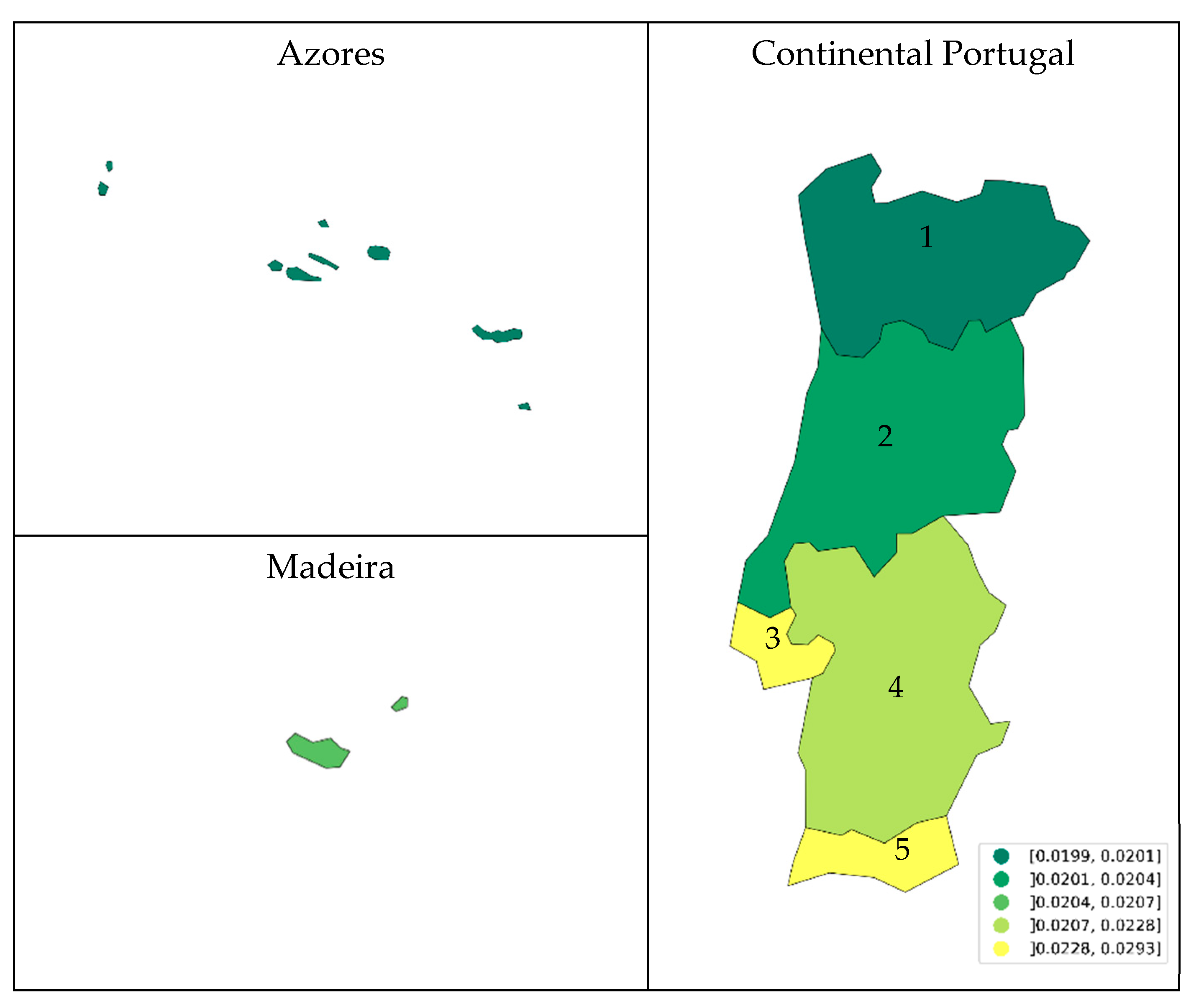
Figure 3), the regions that showed higher GDP per capita were the metropolitan area of Lisbon and the Algarve. These results can be explained by the attractiveness of these regions due to migration movements and employment offers and as a result higher GDP per capita. In the metropolitan area of Lisbon, are located many of the main companies and governmental institutions, leading to a higher GDP per capita.
The NUTS 2 regions of the EU with higher percentages of the population with tertiary education (
Figure 4) were mainly some of the regions in Scandinavia, some regions in France, Spain, Ireland, the Netherlands, and Belgium. In the Portuguese NUTS 2 regions, the regions with higher percentages of tertiary education were the metropolitan area of Lisbon and the center (
Figure 5). The presence of some of the most relevant public universities in those regions contributed to the results.
2.2. Data Envelopment Analysis (DEA)
The DEA is a non-parametric methodology based on mathematical programming models, first developed by Charnes et al. [
16], and aims to study and compare the efficiencies of Data Management Units (DMUs). In this study, the EU NUTS 2 regions are considered the DMUs, the input is the percentage of people with tertiary education, and the output is the variable GDP per capita. This methodology does not consider prior assumptions linking inputs and outputs, and a piecewise linear benchmark frontier is built for the reference practices considering the observed inputs and outputs and how more distant the observations are from this frontier, less efficient they are (closer to 0, less relative performance; Cooper et al. [
17] and Cook and Seiford [
18]). The primal problems define several maximization problems equal to the number of DMUs considered of the ratios between the weighted outputs and the weighted inputs (CRS, constant returns to scale) constrained by these ratios not being greater than 1 for all DMUs, having as decision variables the weights for inputs and outputs. Additionally, the weighted inputs can be constrained to be equal to 1, and the multiplier form of DEA is obtained.
The Pareto–Koopmans efficiency occurs when it is not possible to improve the objective function in terms of inputs or outputs without deteriorating other input(s) or output(s). In practice, the envelopment is built with the dual formulations of these sets of problems. The VRS (variable returns to scale) of these problems is obtained when constraints to a convex combination of input(s) and output(s) are added—expression (4). In this set of dual problems where the output level of GDP per capita is fixed and the percentage of people with tertiary education as input is minimized, the problem is input-oriented, otherwise, it would be output-oriented. The objectives of the set of problems that are to be solved are represented in expression (1). Expression (2) represents the outputs constraints (is the scalar value for the output i, while GDPPC is the vector of all 238 output values), whereas expression (3) represents the inequation for the inputs ( is the scalar value for input i, while TE is the vector of all 238 input values). Expression (5) represents the signal constraints for the dual decision variables for each of the 238 problems. In the case of this work, (efficiency) is a scalar and α is a vector with 238 scalars (multipliers).
For NUTS 2 regions,
i = 1, …, 238
The results of the optimization process show the regions which are technically and mix efficiently by analyzing the input and output slacks, the value of the efficiency decision variable, and the multiplier vector values. Efficiency means how much is needed to multiply the input to be 100% efficient. The scale efficiency is measured by the ratio between VRS input-oriented model efficiency and CRS input-oriented model for each NUTS 2 region. The interested reader can see Ray [
19] for more details about the DEA methodology.
2.3. Spatial Analysis
An exploratory spatial analysis was developed based on the Tobler distance, considering a threshold of 9000 km and a squared inverse distance. Following the Tobler distance for calculating the weights, all regions’ NUTS 2 values of GDP per capita depend on each other, but the closer they are, the more similar they become (and higher the weights [
20]). Ideally, other more suitable methodologies for calculating the weights matrix should be considered, such as the matrices based on the Queen contiguity matrix or the Rook contiguity matrix [
21], but as EU NUTS 2 have some islands, they cannot be considered in this case. These consider the GDP per capita values for NUTS 2 regions more spatially correlated with regions that share a border or a point. However, as this study encompasses regions in islands and isolated in other continents (South America, Africa), they are not appropriate for further analysis.
As measures of spatial exploratory analysis, this work used Moran’s spatial autocorrelation coefficient which means and tests under the null hypothesis whether the NUTS 2 regions do not have spatial autocorrelation (if they are independent) and the LISA (Local Indicator of Spatial Association) cluster that groups statistical significative regions with neighbors (spatial lags) in four clusters: regions and their neighbors with higher values of GDP per capita; regions with higher values with neighbors with lower values of GDP per capita; regions with lower values with neighbors with higher values of GDP per capita; regions and neighbors with lower values of GDP per capita.
2.4. Spatial Regression Modeling
A spatial regression estimation was applied to better understand the relationship between the GDP per capita levels in EU NUTS 2 regions and the percentages of people with tertiary education in those regions. Anselin [
22] suggested the use of the best optimal estimator as the spatial two-stage least squares, avoiding the inverse spatial weights matrix and exploiting the usual series expansion of instruments from the first stage estimation with the robust matrix of White for estimating the model’s covariance matrix. It used the optimal number of spatial lags in the first stage to maximize the determination coefficient of the second-stage regression and at the same time minimize the mean square error of the second-stage regression. The model used is defined by Equations (6) and (7):
where
is the spatial lag which maximizes the regression
and minimizes the mean square error of the regression at the same time. In other words, the lag starts with 1 and at each increment of 1, whether the
is increased and the mean square error is decreased is tested.
represents the GDP per capita for each region,
represents the percentage of tertiary education for each region, and
means the estimated value of the first stage equation based on Equation (7), where W stands for the spatial lag neighborhood matrix.
3. Results
Regarding
Figure 2,
Figure 3,
Figure 4 and
Figure 5, it can be observed that in some EU NUTS 2 regions, high levels of tertiary education correspond to high values of GDP per capita. By opposition, in other regions, low levels of tertiary education correspond to low values of GDP per capita. These cases may correspond to efficient and benchmark-efficient regions when the minimum level for tertiary education is considered, given the values of GDP per capita.
Figure 6 represents the best linear and quadratic fit for the relationship between tertiary education and GDP per capita. It is not very clear that the relationship between the levels of tertiary education and GDP per capita is linear. It also indicates that the CRS DEA model should be chosen or otherwise it is increasing, and we should choose the VRS DEA model. Therefore, both models are analyzed. There are also the IRS (increasing returns to scale) and the DRS (decreasing returns to scale) models, but it was decided to use the VRS model for both situations that can happen in this work; in this case we try to adjust for the best fit of a polynomial curve with a higher degree in
Figure 6 [
23,
24].
Figure 7 shows that the most efficient regions for constant returns to scale with efficiencies greater than about 50% are located in the north of Italy, central European regions, Romania, and Ireland. Some of these regions reached high values of the GDP per capita and high levels of tertiary education as the regions in Ireland and the regions in central Europe. Aside from this, in the case of some Italian regions, we have the correspondence of medium-low levels of tertiary education to medium-high levels of GDP per capita in the EU (and Italy) context.
For the concrete case of Portuguese NUTS 2 regions,
Figure 8 shows that all regions are less than half efficient compared to the EU benchmark. With low values of GDP per capita and low levels of tertiary education, the Azores became the more efficient region in 2020, followed by Alentejo and Algarve. Even though, Alentejo and Algarve have higher values than the Azores for both indicators. The remaining Portuguese regions were about 0.30 efficient.
When considering variable returns to scale (in the VRS model;
Figure 9), the most efficient regions are spread out by Italy, central Europe (Luxembourg, Germany), Romania, and Ireland. In the case of Ireland and some regions in central Europe, the efficiency is higher due to high levels of tertiary education combined with high values of GDP per capita. On the other hand, some Italian regions do not have high percentages of tertiary education when compared with other regions of the EU and have medium-high values of GDP per capita in the EU context. For Romania, regions reach high values for efficiency because they have generally low percentages of the population with tertiary education and relatively medium-low values of GDP per capita.
All Portuguese regions reached efficiency levels when compared with the EU benchmark regions lower than 0.90 (
Figure 10). The analysis is very similar to the CRS model, but with higher levels of efficiency, ranging in the VRS model from about 0.40 to about 0.86.
The model in VRS and the output slacks analysis in
Figure 11 reveal, for some Bulgarian regions (such as Severozapaden, Yugoiztochen, and Severen tsentralen), high values of GDP per capita, given the benchmark and concerning for the input (percentages of tertiary education in their populations).
The VRS considers that the percentages of tertiary education in EU regions are balanced and adequate considering the benchmark and optimization process. For the given GDP per capita levels in none or a few regions, the percentage of tertiary education exceeded the needed for the efficiency of the VRS model.
Figure 12 shows regions with higher scale efficiency values, with some in the north of Italy and central and northern Europe (namely Scandinavian regions). Concerning
Figure 12, the Portuguese region considered more scale-efficient in 2020 is the metropolitan area of Lisbon, followed by the Algarve. The position of the metropolitan area of Lisbon is easy to explain because it has the highest values in Portugal for both indicators (GDP per capita and percentage of tertiary education in population). As was noticed before, they are regions attractive for migrants and have a considerable number of job offers, some in the tertiary sector. In the concrete case of Lisbon, some of the biggest private and public companies have their headquarters there as well as some of the biggest universities and polytechnic institutes, facilitating access to tertiary education and creating job opportunities and consequently a higher GDP per capita (in agreement with [
25,
26]).
The metropolitan area of Lisbon is a Portuguese region with a higher scale efficiency value, followed by the Algarve region (
Figure 13). As observed before, the metropolitan area of Lisbon showed high values of GDP per capita and the percentage of tertiary education in the population. Both regions generally attract migrants and offer job opportunities; some of them linked with tourism and services because in the case of Lisbon there is a concentration of companies and governmental and public institutions (including universities). This concentration helps to explain the higher values of GDP per capita and population with tertiary education.
After analyzing the EU regions’ NUTS 2 efficiencies with Data Envelopment Analysis (DEA) techniques, a neighborhood matrix W for GDP per capita with the distance based on Tobler methodology with a threshold of 9000 km to guarantee that all regions have neighbors and the inverse of Euclidian distance was estimated. This gravitational methodology revealed a spatial correlation of 0.241 and was significant (
p-value = 0.001). Therefore, the hypothesis of the inexistence of spatial autocorrelation is rejected. In
Figure 14, it can also be seen that there are a considerable number of regions with high values of GDP per capita with neighbor regions with high values of GDP per capita (in the first quadrant), a considerable number of regions with low values of GDP per capita with neighbor regions with low values of GDP per capita (in the third quadrant), and some with high values with neighbors with low values (and vice versa; in the second and fourth quadrants), confirming the significant value for the spatial autocorrelation. The paper of Arbia and Piras [
27] confirms the convergence among EU countries with significant and positive spatial autocorrelations for the most recent years studied for GDP per capita values (in agreement with [
28,
29]).
The neighbor matrix W is used to estimate a spatial two-stage least squares model, using the optimal number of spatial lags of the values for tertiary education as the series expansion of instruments in the first stage estimation. The number of lags that minimizes the mean square error and at the same time maximizes the determination coefficient (R2) is considered. The results (
Table 1) show that all coefficients were considered statistically different from zero with an error type I of less than 1%. The Anselin–Kelejian test shows that there is no spatial autocorrelation in the residuals of the model, and it can be said that the variance of GDP per capita is about 43% explained by the variation in independent variables in the model. The spatial two-stage least squares model aims to explain the GDP per capita using the GDP per capita of neighbor regions and the spatially lagged variables of tertiary education (W_TERT_EDU2020 with an optimal 48 spatial lags) in the first stage.
A LISA cluster analysis (
Figure 15) was used, where some regions and respective countries with local spatial autocorrelations statistically different from zero with a significance of 5% were identified, following the gravitational methodology. Represented in the color red are the regions where the GDP per capita reach high values and their neighboring regions also do. In light blue, the regions with low values of GDP per capita and respective lagged regions with high values of GDP per capita are represented. While dark blue represens the regions with low values of GDP per capita and with spatial lags with low values as well.
Figure 15 shows the intervals (groups or clusters) for residuals from the spatial two-stage least squares using positive and negative factors of distances with the residuals’ standard deviations. When we try to compare
Figure 15 with
Figure 16, we can observe that the higher (positive) residuals correspond to clusters of regions with higher values of GDP per capita, while lower (negative) residuals generally correspond to clusters of regions with lower values of GDP per capita.
Furthermore, the spatial two-stage least squares model was the most efficient model when comparing the values of mean square error of spatial two-stage least squares with other models such as the ordinary least squares or the generalized method of moments for a spatial lag and error model. When observing their residuals, it seems that they cannot be considered white noise and they can be heteroskedastic, as we can observe in
Figure 17.
4. Discussion and Conclusions
This study aims to develop a spatial and econometric analysis to explain the GDP per capita and its variations among the EU NUTS 2 regions, using as independent variables the percentage of tertiary education and the spatial lag of the dependent variable, estimated in the first stage with the optimum number of spatial lags (48) taking into consideration the minimum of mean square error and at the same time the maximum of the Pseudo R-squared.
The results show the good adequacy of this modeling approach to explain the variations in GDP per capita among regions. The residuals of the model and its standard deviation were used to classify the regions into more homogeneous groups, which in most cases match the clusters (groups) identified by LISA cluster analysis with the highest and lowest values of GDP per capita.
Previous studies mentioned in the introduction [
4,
5,
6,
7,
8] supported the influence of education on the economy and the product of countries and regions, but this study analyzed not only the regional differences within the countries and the regions, but also the countries where the influence of the percentages of people with tertiary education efficiently and significantly influenced the levels of GDP per capita. For this purpose, firstly, a DEA analysis was developed that highlights the most efficient countries and regions considering as input, the percentage of tertiary education, and as output, the values of GDP per capita. Secondly, a spatial two-stage least squares model (GDP per capita as a dependent variable) was developed with an optimal choice of spatial lags of instrumental variable in the first stage. Afterward, the regions were grouped according to the values of the residuals of the adjusted spatial regression (classes of variation defined by positive and negative variations in residuals’ standard deviations). Finally, the LISA clusters produced from the spatial-lagged GDP per capita were compared with the groups produced by the classes calculated considering the values of the spatial regression standard deviations. Nevertheless, and after revealing the low capacity of explanation of the variation in GDP per capita using the spatial regression model, the model seems adequate and significant for explaining the differences in GDP per capita among NUTS 2 regions caused by the percentage of tertiary education. This same conclusion might be undertaken in the same regions with the DEA optimization analysis as well.
Similarly to Nowak and Dahal [
13], the percentage of tertiary education positively impacts the value of GDP per capita in EU NUTS 2 regions. Therefore, it is recommendable to give special priority to education and science in public policies and the government budget, discouraging the drop-out rate and promoting the universalization of higher education.
Moreover, the analysis of the two-stage least squares model’s residuals’ classes using the standard deviation reveals similar ideas according to previous analysis with DEA optimization. That is, there are some regions with higher values of GDP per capita than expected given their modest literacy level measured by percentages for tertiary education, namely some regions in Italy, Portugal (e.g., Alentejo and Azores), and Bulgaria. On the other hand, there are regions with high levels of literacy (e.g., some in the north of Spain and France) and poorer-than-expected levels of GDP per capita reflected by the econometric model’s residuals’ classes and DEA optimization methodology.
All the modeling techniques used in this work are generally useful to obtain similar and confirmatory conclusions. The case study of Portugal is illustrative and more intuitive for confirming, validating, and analyzing the country regions from which the authors better understand the data. Results are relevant for the metropolitan area of Lisbon and, as we saw in the results section, this region is characterized as being more demographically attractive when compared to other Portuguese regions which can be a consequence of containing the political and governmental capital of Portugal, some of the Portuguese main universities, and the headquarters of most of the important companies in the country. Therefore, it generates a considerable number of job opportunities, attracting the population mainly to the neighboring municipalities around Lisbon and on the margins of the Tagus River.
In future work, more explanatory variables in the spatial regression model may be included. Moreover, it can be applied to spatial and temporal models. However, for that, collecting further data will be needed, and sometimes the regional data are not easily comparable because NUTS 2 regions frequently change the territories’ configurations and their denominations in some countries of the EU.


