An Effective Online Sequential Stochastic Configuration Algorithm for Neural Networks

Abstract

Random Vector Functional-link (RVFL) networks, as a class of random learner models, have received careful attention from the neural network research community due to their advantages in obtaining fast learning algorithms and models, in which the hidden layer parameters are randomly generated and remain fixed during the training phase. However, its universal approximation ability may not be guaranteed if the random parameters are not properly selected in an appropriate range. Moreover, the resulting random learner’s generalization performance may seriously deteriorate once the RVFL network’s structure is not well-designed. Stochastic configuration (SC) algorithm, which incrementally constructs a universal approximator by obtaining random hidden parameters under a specified supervisory mechanism, instead of fixing the selection scope in advance and without any reference to training information, can effectively circumvent these awkward issues caused by randomness. This paper extends the SC algorithm to an online sequential version, termed as an OSSC algorithm, by means of recursive least square (RLS) technique, aiming to copy with modeling tasks where training observations are sequentially provided. Compared to the online sequential learning of RVFL networks (OS-RVFL in short), our proposed OSSC algorithm can avoid the awkward setting of certain unreasonable range for the random parameters, and can also successfully build a random learner with preferable learning and generalization capabilities. The experimental study has shown the effectiveness and advantages of our OSSC algorithm.

1. Introduction

Neural networks have received careful attention with the development of artificial intelligence by virtue of their ‘black-box’ capability in model approximation via a data-driven manner [1,2,3,4]. It commonly known that the primary way for training a neural network with fixed architecture is the back-propagation (BP) algorithm, which has become one of the main driving forces in deep learning domains [5]. However, it is generally accepted that the BP algorithm has certain drawbacks in different perspectives: (1) the effectiveness of the BP algorithm to some extent relies on the design of network architecture. However, it is generally difficult to predefine an optimal architecture for a given task. The commonly used way for designing the network architecture is the trial-and-error method, which is time-consuming and potentially impacts the effectiveness of the resulting model; (2) it suffers from several issues such as the weight initialisation, local minima, and sensitivity of the learning performance with respect to the learning rate setting. Empirically, this gradient-based learning method could not produce meaningful or interpretable internal representations from each hidden outputs [6]; (3) it usually tends to be trained slowly when all of the neural network parameters must be iteratively tuned from scratch.

Randomized algorithms for training neural networks have been explored and developed since the 1980s [7,8] and well discussed in the early- to mid-1990s [9,10,11,12,13]. It is empirically verified that neural networks with random weights (NNRWs) are computationally efficient since their input weights are randomly assigned and remain fixed during the training process. There are many different formulation/concepts related to NNRWs [14,15], such as Random Vector Functional-link (RVFL) network [11,12,13], Random Kitchen Sinks (RKS) [16], Random Features for Kernel Machines (RFKM) [17], Stochastic Configuration Networks (SCN) [18], etc. A fundamental issue for NNRWs is that of whether or in which perspective the randomized learner model has universal approximation capability (UAC), which is the most important theoretical basis for algorithm implementation. In particular, the UAC of RVFL networks has been theoretically verified in [13] and further refined in [19]. Both the approximation and estimation error bounds are proved for RKS in [16]. These theoretical results, however, only ensure that there exists suitable random distribution $\mathcal{P}$ such that a randomized neural network with the weights and biases randomly selected from $\mathcal{P}$ has universal approximation capability in the sense of probability. Given a training dataset, as for the algorithm implementation in practice, it is not trivial to set a proper distribution (range) for problem solving. In other words, once the random distribution is not reasonably pre-defined, the universal approximation of the randomized neural network model cannot be ensured [20,21,22]. To the best of our knowledge, SCN [18] is the first work that constructs effective NNRWs by stochastically configuring the hidden weights and biases according to a data-dependent supervisory mechanism. Importantly, the universal approximation theory of SCN is guaranteed in a deterministic way, and, in comparison with RVFL networks, its favorable capability and good potential in dealing with both regression and classification problems has been well verified in various scenarios [23,24,25,26,27,28]. In this work, therefore, we focus on the extension of SCN, and the RVFL network is considered as a baseline.

In some domains, such as industry, finance, meteorology, etc., the data samples are collected in a sequential/streaming manner, that is, samples are available via the one-by-one or chunk-by-chunk way. In addition, in some applications, batch learning algorithms are not suitable, as the process of retraining, whenever new data are received, is impractical for problem-solving. Under this problem formulation, in this paper, we aims to further extent the framework of SCN, which is formulated in batch mode (i.e., considering all the available data at once), to be capable for building randomized neural networks with sequential training data. In particular, an effective Online Sequential Stochastic Configuration (OSSC) algorithm is proposed for problem-solving. The whole process of the OSSC algorithm can be formulated by two main steps: (i) initialization phase, where the stochastic configuration algorithm [18] is applied to construct a base (initial) random learner model with generally acceptable (initial) approximation error; (ii) sequential updating phase, where the widely-used recursive least square (RLS) approach is performed for the purpose of renewing recursively the output weights of the initial model. The algorithmic convergence can be guaranteed, provided that the initialization phase is successfully processed. To highlight the effectiveness of OSSC, we also summarize some remarks to present the advantages of OSSC over the baseline OS-RVFL (i.e., a straightforward/trivial extension of RVFL network to its online sequential learning version). Extensive experimental studies, including two synthetic examples for 1D function approximation, one example for nonlinear dynamic system modeling, one example of Mackey–Glass time-series prediction, and one case study for foreign exchange rate forecasting application, are conducted to demonstrate the merits of our proposed OSSC, in comparison with OS-RVFL. We also provide a robustness analysis to study empirically the influence of chunk size on the model’s performance. All of the experimental results show clearly the fact that OSSC is effective and has a good potential for dealing with sequential data modeling tasks.

In summary, our contributions are as follows:

• An effective Online Sequential Stochastic Configuration (OSSC) algorithm is proposed for training neural networks with sequential training data. As a favorable randomized learner model, OSSC further supplements the variants of SCNs [18];
• Based on the extensive experimental studies, where OSSC is compared with OS-RVFL on several online learning tasks, we uncover certain uncertainty issues and also provide some useful clues, which are empirically beneficial for interested readers to have a clear and accurate understanding about developing online version of neural networks with random weights.

The remainder of this paper is organized as follows: Section 2 briefly reviews RVFL networks. Section 3 recalls the stochastic configuration framework with both theoretical and algorithmic description. An effective Online Sequential Stochastic Configuration (OSSC) algorithm is proposed in Section 4. Extensive experimental investigations are provided in Section 5. Finally, Section 6 concludes this work and gives further expectations for future work.

2. Basics of RVFL Networks

RVFL networks can be treated as a class of random learner models with a remarkable feature that the input weights and biases are randomly selected and remain fixed during the training phase. In this paper, we only consider RVFL networks without a direct link from the input to the output, which is equivalent to a single hidden layer feedforward neural network (SLFN) that can be mathematically described as

$$G_L(\mathbf{x};w,b)=\sum _{j=1}^L{\beta }_{j}g(w_j^{\mathrm{T}}\mathbf{x}+b_j),$$

where L is the number of hidden nodes, $\mathbf{x}={[x_1,x_2,\dots ,x_d]}^{\mathrm{T}}\in {\mathbb{R}}^d$ is the input vector, g is the activation function, $b_k\in \mathbb{R}$ is the bias, $w_j={[w_{j1},w_{j2},\dots ,w_{jd}]}^{\mathrm{T}}\in {\mathbb{R}}^d$ is the input weight, ${\beta }_j\in \mathbb{R}$ is the output weight connecting the j-th hidden node and the output node. Now, we briefly describe the learning process for RVFL networks. Assume that we are given a training set $\{{\mathbf{x}}_i,t_i\}$ with N samples of the target function ($i=1,2,\dots ,N$), ${\mathbf{x}}_i\in {\mathbb{R}}^d$, $t_i\in \mathbb{R}$. Remember that $w_k$ and $b_k$ are randomly selected and fixed in the training phase; therefore, the learning objective is to solve the following optimization problem:

$$\underset{{\beta }_1,\dots ,{\beta }_j}{min}\sum _{i=1}^N{\left(\sum _{j=1}^L{\beta }_{j}g(w_j^{\mathrm{T}}{\mathbf{x}}_i+b_j)-t_i\right)}^2,$$

which is equivalent to a standard least square (LS) problem

$${\beta }^{*}=arg\underset{\beta \in {\mathbb{R}}^L}{min}{\parallel H\beta -T\parallel }_2^2$$

where

$$H=\left(\begin{array}{ccc}g(w_1^{\mathrm{T}}{\mathbf{x}}_1+b_1)& \cdots & g(w_L^{\mathrm{T}}{\mathbf{x}}_1+b_L)\\ ⋮& \cdots & ⋮\\ g(w_1^{\mathrm{T}}{\mathbf{x}}_N+b_1)& \cdots & g(w_L^{\mathrm{T}}{\mathbf{x}}_N+b_L)\end{array}\right)$$

is the hidden layer output matrix, $T={[t_1,t_2,\dots ,t_N]}^{\mathrm{T}}$, $\beta ={[{\beta }_1,{\beta }_2,\dots ,{\beta }_L]}^{\mathrm{T}}$. Finally, a close form solution of the output weights can be obtained by using the pseudo-inverse method, i.e., ${\beta }^{*}=H^{†}T$.

In passing, the universal approximation theorem of RVFL networks [13,19] can only ensure that there exists a certain appropriate range for randomly assigning the hidden parameters rather than totally independent with the training information, indicating the fact that the random selection scope for the input weights and biases has a significant impact on the random learner’s performance. In other words, a trivial range $[-1,1]$ for randomly assigning input weights and biases may fail in leading to a universal approximator. Indeed, an inappropriate selection scope from which the hidden parameters are randomly generated will incur very bad learning and generalization performance. Li and Wang [21] have addressed some ‘risky’ aspects caused by the randomness, revealing some practical issues and pitfalls when using this kind of random learner model. These ‘risky’ aspects may still exist and/or cause outrageous results in the process of applying a sequential learning framework for RVFL networks, in the case that training observations are sequentially provided. This motivates us to find a better online learning system by reconsidering the stochastic configuration algorithm that has sufficient effectiveness in constructing a random learner with good learning and generalization capabilities [18], as delineated in the next section.

3. Revisit of the Stochastic Configuration Algorithm

In [18], stochastic configuration algorithms were proposed to circumvent those awkward issues in applying RVFL networks, by incrementally constructing an universal approximator with random hidden parameters found on the basis of specified supervisory mechanism. The selection scope for the hidden parameters is determined randomly but with an objective to decrease the residual error incrementally, instead of being fixed in advance. The simulation results in [18] have shown the merits of the SC algorithm in comparison with some existing RVFL-based randomized algorithms.

Here, we revisit the constructive process of the SC framework, followed by the restatements of both the theoretical and algorithmic results. Let $L_2\left(D\right)$ denote the space of all Lebesgue-measurable vector-valued functions $f:{\mathbb{R}}^d\to \mathbb{R}$ on a compact set $D\subset {\mathbb{R}}^d$, with the $L_2$ norm defined as ${\parallel f\parallel }_2:=({\int }_D{\left|f\left(x\right)\right|}^2{dx)}^{1/2}<\infty$. For a target function $f:{\mathbb{R}}^d\to \mathbb{R}$, assume a single layer feed-forward network (SLFN) with $L-1$ hidden nodes ($L=1,2,\dots$) have already been constructed, that is, $f_{L-1}\left(x\right)={\sum }_{j=1}^{L-1}{\beta }_j{g}_j(w_j^{\mathtt{T}}x+b_j)$ ($f_0=f$). If the current residual error denoted as $e_{L-1}=f-f_{L-1}$ is still unacceptable, the SC framework is concerned with how to add ${\beta }_L$, $g_L$ ($w_L$ and $b_L$) leading to $f_L=f_{L-1}+{\beta }_L{g}_L$ until the residual error $e_L=f-f_L$ is suitable for the given task, that is, $\parallel e_L\parallel$ is smaller than an expected specific tolerance $ϵ$.

Theorem 1

([18]). Given that span (Γ) is dense in $L_2$ and $\forall g\in \mathsf{\Gamma }$, $0<\parallel g\parallel <b$ for some $b\in {\mathbb{R}}^{+}$. Given $0<r<1$ and a nonnegative real number sequence, $\left\{{\mu }_L\right\}$ with ${lim}_{L\to +\infty }{\mu }_L=0$ and ${\mu }_L\le (1-r)$. For $L=1,2,\dots$, denote a factor

$${\delta }_L=(1-r-{\mu }_L){\parallel e_{L-1}\parallel }_2^2>0.$$

(1)

If $g_L$ is selected to satisfy

$${\langle e_{L-1},g_L\rangle }^2\ge b^2{\delta }_L^{*},$$

(2)

and

$${\mathit{\beta }}^{*}=arg\underset{\beta }{min}{\parallel f-\sum _{j=1}^L{\beta }_j{g}_j\parallel }_2$$

(3)

then

$$\underset{L\to +\infty }{lim}{\parallel f-f_L^{*}\parallel }_2=0,$$

where $f_L^{*}={\sum }_{j=1}^L{\beta }_j^{*}{g}_j$.

Given a training set with inputs $X=\{x_1,x_2,\dots ,x_N\}$, $x_i={[x_{i,1},\dots ,x_{i,d}]}^{\mathrm{T}}\in {\mathbb{R}}^d$ and outputs $T={[t_1,t_2,\dots ,t_N]}^{\mathrm{T}}$, $i=1,\dots ,N$. We denote $e_{L-1}\left(X\right)={[e_{L-1}\left(x_1\right),\dots ,e_{L-1}\left(x_N\right)]}^{\mathrm{T}}\in {\mathbb{R}}^N$ as the corresponding residual error vector before the L-th new hidden node is added. The hidden layer output matrix (with L hidden nodes) can be formulated as $H^{\left(L\right)}=[h_1,h_2,\dots ,h_L]$, where $h_L\left(X\right)={[g_L(w_L^{\mathrm{T}}{x}_1+b_L),g_L(w_L^{\mathrm{T}}{x}_2+b_L),\dots ,g_L(w_L^{\mathrm{T}}{x}_N+b_L)]}^{\mathrm{T}}$ is the activation of the new hidden node for each input $x_i$, $i=1,2,\dots ,N$. In practice, we use ${\xi }_L=({(e_{L-1}{\left(X\right)}^{\mathrm{T}}·h_L\left(X\right))}^2/(h_L{\left(X\right)}^{\mathrm{T}}·h_L\left(X\right))-(1-r-{\mu }_L)e_{L-1}{\left(X\right)}^{\mathrm{T}}{e}_{L-1}\left(X\right))$ as a consistent estimate version of Equation (2). With these notations, the detailed stochastic configuration algorithm [18] is summarized as the following Algorithm 1.

Algorithm 1: SC

Given inputs $X=\{x_1,x_2,\dots ,x_N\}$, $x_i\in R^d$ and outputs $T=\{t_1,t_2,\dots ,t_N\}$, $t_i\in \mathbb{R}$. Set maximum number of hidden neurons $L_{max}$, expected error tolerance $ϵ$, maximum times of random configuration $T_{max}$. Choose $0<r<1$, and a set of the scale parameters $\mathsf{{\rm Y}}\doteq \{{\lambda }_1:\Delta \lambda :{\lambda }_{max}\}$ in sigmoid

1. Initialize $e_0:={[t_1,t_2,\dots ,t_N]}^{\mathtt{T}}$, denote two empty sets $\mathsf{\Omega }$ and W;

2. For$L=1,2,\dots ,L_{max}$, Do

3. For$\lambda \in \mathsf{{\rm Y}}$, Do

4.  For$k=1,2\dots ,T_{max}$, Do

5.   Randomly select ${\omega }_L$ and $b_L$ from ${[-\lambda ,\lambda ]}^d$ and $[-\lambda ,\lambda ]$

6.    Calculate $h_L$ and ${\xi }_L$. Set ${\mu }_L=\frac{1-r}{L+1}$

7.     If${\xi }_L\ge 0$

8.      Save$w_L$ and $b_L$ in W, ${\xi }_L$ in $\mathsf{\Omega }$, respectively;

9.     Else go back to Procedure 4

10.   End For (corresponds to Procedure 4)

11.   IfW is not empty

12.     Break

13.   End If

14. End For (corresponds to Procedure 3)

15. IfW is empty

16.   Reset$r:=r+(1-r)/2$ and return to Procedure 3;

17. Else find $w_L^{*}$, $b_L^{*}$ that maximize ${\xi }_L$ in $\mathsf{\Omega }$

18. Calculate $H^{\left(L\right)}$, ${\beta }^{*}={\left(H^{\left(L\right)}\right)}^{†}T$, and $e_L=e_{L-1}-{\beta }_L^{*}{h}_L^{*}$

19. If$\parallel e_L{\parallel }_2\le ϵ$

20.  Return${\beta }^{*}$, ${\omega }^{*}$, and $b^{*}$;

21. Else go back to Procedure 2

22. End For (corresponds to Procedure 2)

It should be noted that the vanilla version of the Algorithm 1 is a batch mode that considers all the available data at once during the training process, which in other words can be viewed as a batch learning algorithm. However, when new data samples are received, one needs to retrain the whole model from scratch using the SC algorithm again, which is impractical for some real-world applications with special concerns on real-time processing. For problem-solving, it is necessary to extend the current Algorithm 1 to a more advanced one that supports sequential learning, which allows iteratively updating the model’s trainable parameters (on the basis of the parameters obtained in the last iteration session), instead of retaining the whole model, when new data samples are available via the one-by-one or chunk-by-chunk way. We detail the proposed new variant of SC algorithm in the following section.

4. Online Sequential Stochastic Configuration Algorithm

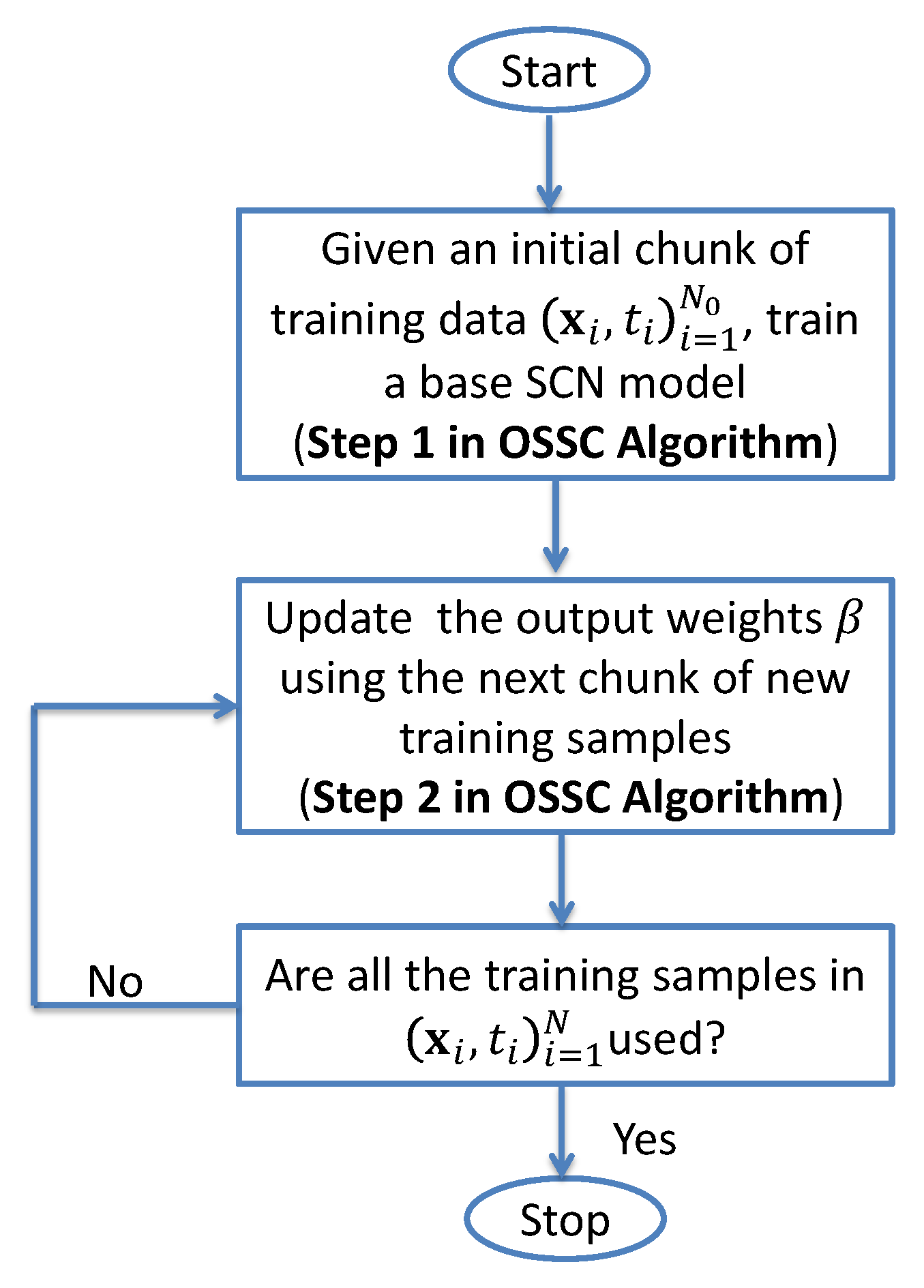
In this section, the SC algorithm is generalized into a sequential learning version, by executing the widely-used recursive least square (RLS) approach. We will first provide the mathematical deduction step by step to finalize the iteration equations for the output weights. Then, the whole procedures are summarized as the Algorithm 2 OSSC, followed by further comments about its inherent superiority over the OS-RVFL algorithm, that is, a similar sequential learning method that uses RVFL networks as a base model during the online training process.

The whole process can be formulated by two main steps including initialization phase and sequential updating phase, where the Algorithm 1 is applied in the first phase and consequently obtains a base (initial) random leaner, and the RSL approach is performed in the second phase for renewing output weights of the initial model, detailed as follows.

Initialization Phase: We use the SC algorithm on the first available training data; suppose that the constructed random learner has L hidden nodes, i.e., $f_L\left(x\right)={\sum }_{j=1}^L{\beta }_j{g}_j(w_j^{\mathtt{T}}x+b_j)$. Let ${\beta }^{\left(0\right)}={[{\beta }_1,\dots ,{\beta }_L]}^{\mathrm{T}}$ be the current output weights. The associated hidden layer output matrix is denoted as $H_0$ (here, we remove its top right corner index L for simplicity, i.e., $H_0=H^{\left(L\right)}$).

Sequential Updating Phase: At time instant $k+1$, $k=0,1,\dots$, suppose the hidden layer output matrix corresponding to the new available data are $H_{k+1}$, then the optimization problem becomes

$$\begin{array}{c}\hfill \underset{{\beta }^{(k+1)}}{min}\parallel \left[\begin{array}{c}{H}_k\\ H_{k+1}\end{array}\right]{\beta }^{(k+1)}-\left[\begin{array}{c}{T}_k\\ T_{k+1}\end{array}\right]{\parallel }_2^2.\end{array}$$

(4)

The RLS approach aims at calculating the weight ${\beta }^{k+1}$ recursively from ${\beta }^{\left(k\right)}$ without directly solving the above minimization problem (4).

It is straightforward to observe that

$$\begin{array}{ccc}\hfill {\beta }^{(k+1)}& =& {\left({\left[\begin{array}{c}{H}_k\\ H_{k+1}\end{array}\right]}^{\mathrm{T}}\left[\begin{array}{c}{H}_k\\ H_{k+1}\end{array}\right]\right)}^{-1}{\left[\begin{array}{c}{H}_k\\ H_{k+1}\end{array}\right]}^{\mathrm{T}}\left[\begin{array}{c}{T}_k\\ T_{k+1}\end{array}\right]\hfill \\ & =& P_{k+1}^{-1}{\left[\begin{array}{c}{H}_k\\ H_{k+1}\end{array}\right]}^{\mathrm{T}}\left[\begin{array}{c}{T}_k\\ T_{k+1}\end{array}\right],\hfill \end{array}$$

where

$$P_{k+1}={\left[\begin{array}{c}{H}_k\\ H_{k+1}\end{array}\right]}^{\mathrm{T}}\left[\begin{array}{c}{H}_k\\ H_{k+1}\end{array}\right].$$

It is easy to find that

$$P_{k+1}=P_k+H_{k+1}^{\mathrm{T}}{H}_{k+1},\mathrm{and}{\beta }^{\left(k\right)}=P_k^{-1}{H}_k^{\mathrm{T}}{T}_k.$$

Thus,

$$\begin{array}{ccc}\hfill {\left[\begin{array}{c}{H}_k\\ H_{k+1}\end{array}\right]}^{\mathrm{T}}\left[\begin{array}{c}{T}_k\\ T_{k+1}\end{array}\right]& =& P_k{\beta }^{\left(k\right)}+H_{k+1}^{\mathrm{T}}{T}_{k+1}\hfill \\ & =& (P_{k+1}-H_k^{\mathrm{T}}{H}_k){\beta }^{\left(k\right)}+H_{k+1}^{\mathrm{T}}{T}_{k+1}\hfill \\ & =& P_{k+1}{\beta }^{\left(k\right)}-H_k^{\mathrm{T}}{H}_k{\beta }^{\left(k\right)}+H_{k+1}^{\mathrm{T}}{T}_{k+1}.\hfill \end{array}$$

Then,

$$\begin{array}{ccc}\hfill {\beta }^{(k+1)}& =& P_{k+1}^{-1}(P_{k+1}{\beta }^{\left(k\right)}-H_k^{\mathrm{T}}{H}_k{\beta }^{\left(k\right)}+H_{k+1}^{\mathrm{T}}{T}_{k+1})\hfill \\ & =& {\beta }^{\left(k\right)}+P_{k+1}^{-1}{H}_{k+1}^{\mathrm{T}}(T_{k+1}-H_{k+1}{\beta }^{\left(k\right)})\hfill \end{array}$$

By using the matrix inversion lemma [29], we can obtain that

$$\begin{array}{ccc}\hfill P_{k+1}^{-1}& =& {(P_k+H_{k+1}^{\mathrm{T}}{H}_{k+1})}^{-1}\hfill \\ & =& P_k^{-1}-P_k^{-1}{H}_{k+1}^{\mathrm{T}}{\left(H_{k+1}{P}_k^{-1}{H}_{k+1}^{\mathrm{T}}\right)}^{-1}{H}_{k+1}{P}_k^{-1}.\hfill \end{array}$$

To summarize, let $U_k=P_k^{-1}$, and the online update of the weight can be achieved by the following operation:

$$\begin{array}{ccc}\hfill U_{k+1}& =& U_k-U_k{H}_{k+1}^{\mathrm{T}}{\left(H_{k+1}{P}_k^{-1}{H}_{k+1}^{\mathrm{T}}\right)}^{-1}{H}_{k+1}{U}_k\hfill \\ \hfill {\beta }^{(k+1)}& =& {\beta }^{\left(k\right)}+U_{k+1}{H}_{k+1}^{\mathrm{T}}(T_{k+1}-H_{k+1}{\beta }^{\left(k\right)}).\hfill \end{array}$$

The whole schematic of OSSC algorithm (i.e., Algorithm 2) can be summarized as follows.

Algorithm 2: OSSC

Input: Training dataset arriving sequentially ${\{{\mathbf{x}}_i,t_i\}}_{i=1}^N$, initial number of training samples $N_0$, the number of observations in the k-th chunk, $N_k$.

Output: Output weight $\beta$.

Begin

Step 1. Use the Algorithm 1 on ${\{{\mathbf{x}}_i,t_i\}}_{i=1}^{N_0}$, obtain $H_0$ and ${\beta }^{\left(0\right)},$ set k:= 0;

Step 2. Provide the (k + 1)-th chunk of new observations and calculate $H_{k+1}$ $$\begin{array}{ccc}\hfill P_k& =& H_k^{\mathrm{T}}{H}_k,U_k=P_k^{-1};\hfill \\ \hfill U_{k+1}& =& U_k-U_k{H}_{k+1}^{\mathrm{T}}{\left(H_{k+1}{P}_k^{-1}{H}_{k+1}^{\mathrm{T}}\right)}^{-1}{H}_{k+1}{U}_k;\hfill \\ \hfill {\beta }^{(k+1)}& =& {\beta }^{\left(k\right)}+U_{k+1}{H}_{k+1}^{\mathrm{T}}(T_{k+1}-H_{k+1}{\beta }^{\left(k\right)}).\hfill \end{array}$$  k:= k + 1 and repeat Step 2 until all the observations in ${\{{\mathbf{x}}_i,t_i\}}_{i=1}^N$ are used;

End

The general process of Algorithm 2 (OSSC) is illustrated in the following Figure 1.

Remark 1.

It is easy to find that the whole algorithmic procedures can be immediately used on the original RVFL networks that lead to its online sequential learning version, termed OS-RVFL. That is to say, instead of conducting the SC algorithm in the initialization phase (Step 1 in Algorithm 2), the initial model is offered by implementing the randomized learning algorithm for RVFL networks, i.e., randomly assigning input weights and biases from certain scopes and only optimizing the output weights, as recalled in Section 2. Later for the sequential learning process, the basic iteration procedures remain the same as Step 2 in Algorithm 2.

Remark 2.

The existing convergence results of RLS methodology [30,31] can lend some support to ensure the convergence of our Algorithm 2 (OSSC), provided the initialization phase is successfully processed. In other words, the sequential learning process might be meaningless if the initialization model has not been appropriately trained either due to insufficient training information provided, or because of unreasonable neural network structure and/or parameter setting. On the other hand, for the OS-RVFL algorithm, some undesirable impacts of randomness, for instance, an inappropriate random selection range for input weights and biases, fails in bringing a universal approximator [21], will still exist or be enhanced during the sequential learning phase. That is, the reason why more attention should be raised when applying OS-RVFL for modeling due to the ‘risky’ aspects caused by randomness in RVFL networks.

Remark 3.

Compared with OS-RVFL, our Algorithm 2 (OSSC) incrementally constructs the initial model based on Theorem 1 that can effectively build a random learner with good learning and generalization capabilities. Importantly, the the SC algorithm (i.e., Algorithm 1) performed in the initialization phase can circumvent the awkward setting of the number of hidden nodes, and also find an effective choice of random parameters resulting in a universal approximator on the basis of the first available data. The merits of SC algorithm stated in [18] benefit the following sequential learning processes and bring inherent advantages for OSSC in comparison with OS-RVFL, just like the SC algorithm outperforms the RVFL algorithm shown in [18].

Remark 4.

It should be mentioned that the chunk size, i.e., the number of observations arrived at each time instant, does not necessarily have to be equal. On the other hand, the problem of the minimum number of observations that are needed in the initialization phase is application and problem-dependent. As a whole, the influence of the initial number of observations and the chunk size on the system’s performance should be investigated in depth, as conducted in our experimental study in the next section.

Overall, the key technical differences between OSSC and OS-RVFL (Here, without loss of generality, OS-RVFL represents a broad class of existing models that uses neural networks with random weights assigned via a data-independent manner, which inevitably causes some uncertainly issues as mentioned in the remarks, to name a few) can be summarized as follows in

Table 1. Differences between OSSC and OS-RVFL in terms of several aspects: whether or not the randomness is involved, whether or not stochastic configuration mechanism is used for input weights assignment (term as ‘SC for Random Weights’), whether or not the universal approximation capability (UAC) of base model is guaranteed, and whether or not the convergence property of the online learning process is guaranteed.

Algorithms	Characteristics
	Randomness	SC for Random Weights	Guarantee of UAC	Guarantee of Convergence
OS-RVFL	√	×	×	×
OSSC	√	√	√	√

.

5. Experiments

In this section, we compare the proposed OSSC algorithm with OS-RVFL on different tasks, in order to demonstrate its merits and good potential in dealing with online sequential learning problems. First, we revisit the toy examples used in [21] and change their formulation as a online learning task, by which the advantages of OSSC (over OS-RVFL), which can successfully find some workable random parameters (input weights and biases) and consequently lead to a universal approximator, are illustrated. Then, the effectiveness of our OSSC algorithm is assessed in the problem of nonlinear dynamic system modeling and Mackey–Glass time-series prediction, respectively. In the performance comparison, several scenarios with different parameter settings are performed. Root Mean Square Error (RMSE) that is commonly used in data analysis literature is calculated to measure the performance. Both the average value and standard deviation of RMSE are reported. The parameter setting will be specified in each task. All simulations are carried out in the MATLAB 2020b environment running on a core i7, 2.9 G HZ CPU, and 8 GB RAM.

5.1. 1D Function Approximation

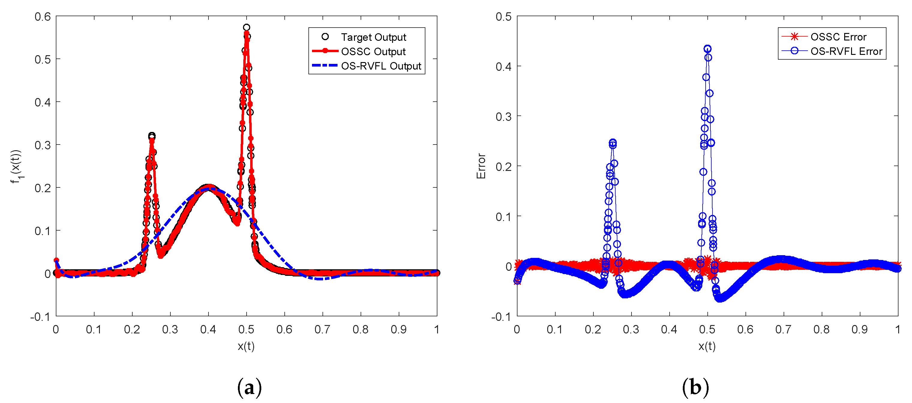
First, to better demonstrate the advantages of OSSC over OS-RVFL with performance visualization, we use two examples for 1D function approximation. In particular, the first regression task is about the followed target function, which has also been used in [21], i.e.,

$$\begin{array}{ccc}\hfill f_1\left(x\right)& =& 0.2e^{-{(10x-4)}^2}+0.5e^{-{(80x-40)}^2}+0.3e^{-{(80x-20)}^2},\hfill \\ \hfill & & x\in [0,1].\hfill \end{array}$$

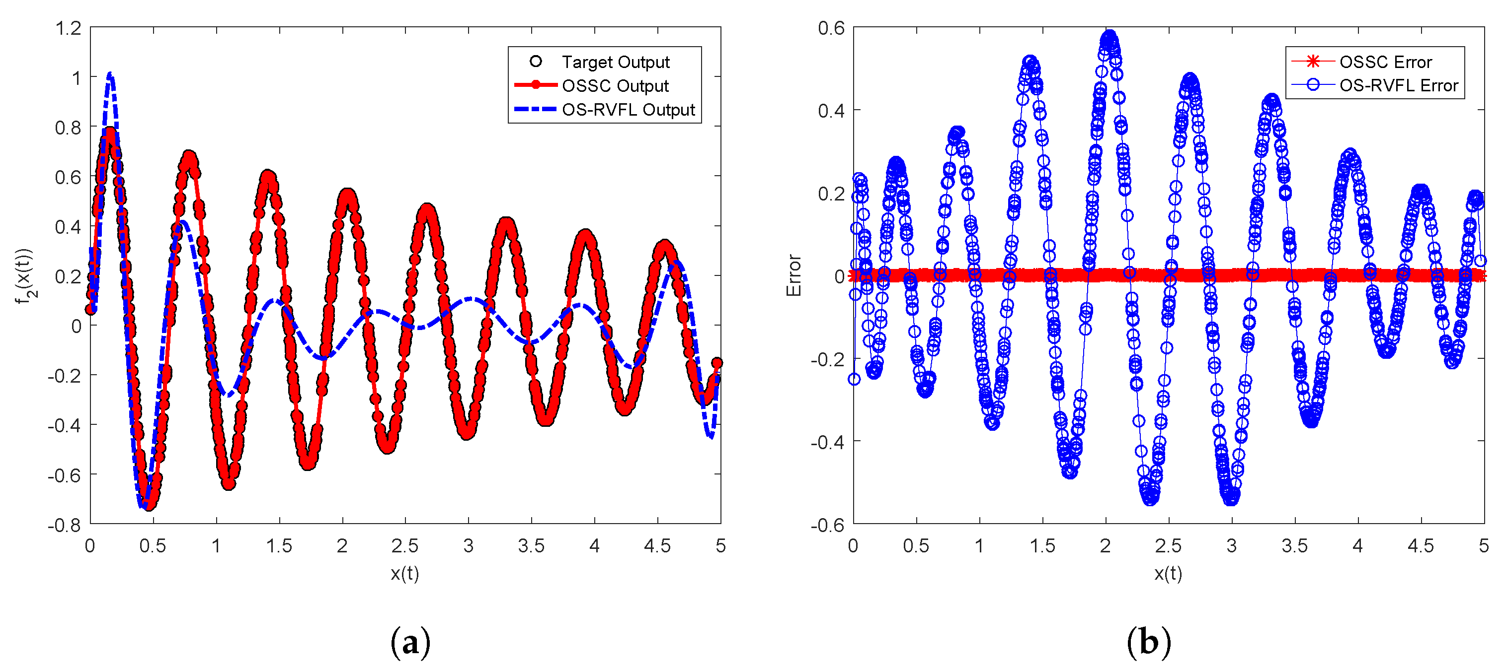
The second target function is a rapidly changing continuous SinE function $f_2$, i.e.,

$$f_2\left(x\right)=0.8exp(-0.2x)sin\left(10x\right),x\in [0,5].$$

To fit the problem formulation of sequential learning task, we sample $N_0=400$ samples as the initial training samples (i.e., $t=0$) and then add training samples sequentially (e.g., 1 by 1, 20 by 20, 50 by 50) as the instances used in training time instants $t=1,2,\dots ,T$, and finally 500 samples as the test samples (which we assume are used for the performance evaluation at the time instant $T+1$).

As shown in

Table 2. Test performance comparison for 1D function approximation Task. MEAN and STD denote the average value and standard deviation of RMSE values.

Datasets	Algorithms	Test Performance with Different Chunk Size (MEAN, STD)
		1 by 1	20 by 20	50 by 50
$f_1$, $N_0=400$, $L=100$	OS-RVFL ($\lambda =1$)	0.0527, 2.9028 × ${10}^{-4}$	0.0527, 2.7041 × ${10}^{-4}$	0.0527, 2.6000 × ${10}^{-4}$
	OS-RVFL ($\lambda =50$)	0.0337, 0.0126	0.0330, 0.0053	0.0329, 0.0057
	OS-RVFL ($\lambda =100$)	0.0406, 0.0447	0.0355, 0.0069	0.0359, 0.0083
	OS-RVFL ($\lambda =200$)	0.0400, 0.0106	0.0416, 0.0079	0.0394, 0.0112
	OSSC	0.0096, 0.0223	0.0087, 0.0094	0.0075, 0.0060
$f_2$, $N_0=400$, $L=50$	OS-RVFL ($\lambda =1$)	0.5165, 1.1486	0.3405, 0.1944	0.4623, 0.9694
	OS-RVFL ($\lambda =5$)	0.1188, 0.2022	0.1084, 0.0865	0.1055, 0.0914
	OS-RVFL ($\lambda =10$)	0.2404, 0.7154	0.3790, 0.1944	0.4623, 0.9694
	OS-RVFL ($\lambda =50$)	0.5165, 1.1486	0.3405, 0.1944	0.4623, 0.9694
	OSSC	8.1488 × ${10}^{-4}$, 0.0013	6.7606 × ${10}^{-4}$, 0.0005	8.8794 × ${10}^{-4}$, 0.0023

, it is clear that OSSC outperforms OS-RVFL in all cases. For example, for the case of $f_1$, the RMSE values of OS-RVFL are larger than $0.03$ in all situations with different settings of $\lambda$ and chunk size. In contrast, the best test result of OSSC is $0.0075$, which means that OS-RVFL’s error is approximately 25 times larger than that of OSSC. This verifies the effectiveness of OSSC as discussed in Remark 2 in Section 4. Approximately, OSSC has obtained 25 times lower RMSE than OS-RVFL. As for $f_2$, the same finding can be obtained, that is, the best test result of OSSC is $8.879e-04$, while the RMSE values of OS-RVFL are all larger than $0.1$. In Figure 2 and Figure 3, for the case of $f_1$ and $f_2$, respectively, we plot the target test outputs, OSSC outputs, OS-RVFL outputs, as well their associated error curves. As can be seen clearly, identical to the findings shown in Table 2, OSSC achieves much better performance than OS-RVFL in both $f_1$ and $f_2$ sequential learning tasks. Obviously, the error curves of OS-RVFL show that the resulting learner models are not well sequentially trained and then do not have acceptable generalization capabilities.

In summary, similar to the findings presented in [21], the random distribution (corresponding to $\lambda$) is of great importance to induce an effective randomized learner model. Furthermore, users should ensure that the initialization phase of online sequential learning can lead to a good initial model; otherwise, the following sequential updating phase is meaningless.

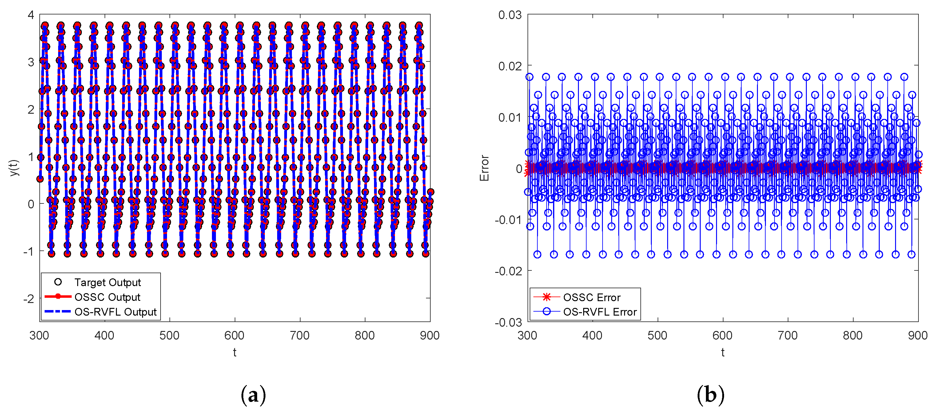
5.2. Nonlinear Dynamic System Modeling

The second task that we consider in our experiments is a nonlinear dynamic system modeling (nDSM) example. In particular, the following artificial example is a widely-used one to demonstrate the neural networks’ feasibility on nDSM:

$$y(t+1)=\frac{y\left(t\right)y(t-1)\left(y\right(t+2.5\left)\right)}{1+y^2\left(t\right)+y^2(t-1)}+u\left(t\right),$$

(5)

where $y\left(1\right)=0$, $y\left(2\right)=0$, $u\left(t\right)=sin(\pi t/25)$.

We compare OSSC and OS-RVFL on this task, in which 900 points are generated using Equation (5) and split into two parts, 300 ($1\le t\le 300$), 600 ($301\le t\le 900$) for training and test, respectively. For either OSSC or OS-RVFL, the inputs used for model training are given by $\left(y\right(t-1),y(t),u(t\left)\right)$ and the corresponding target output is $y(t+1)$.

In

Table 3. Test performance comparison for the nonlinear dynamic system modeling task. MEAN and STD denote the average value and standard deviation of RMSE values.

${\mathit{N}}_0$ Values	Algorithms	Test Performance with Different Chunk Size (MEAN, STD)
		1 by 1	10 by 10	20 by 20	50 by 50
$N_0=100$	OS-RVFL	0.0131, 0.0022	0.0134, 0.0025	0.0137, 0.0026	0.0136, 0.0027
	OSSC	0.0109, 0.0011	0.0111, 0.0012	0.0106, 0.0010	0.0106, 0.0010
$N_0=200$	OS-RVFL	0.0115, 0.0093	0.0099, 0.0012	0.0100, 0.0015	0.0101, 0.0014
	OSSC	0.0076, 6.9002 × ${10}^{-4}$	0.0076, 6.3451 × ${10}^{-4}$	0.0076, 5.3478 × ${10}^{-4}$	0.0077, 6.1279 × ${10}^{-4}$
$N_0=300$	OS-RVFL	0.0100, 0.0014	0.0099, 0.0015	0.0102, 0.0014	0.0103, 0.0015
	OSSC	0.0076, 5.9729 × ${10}^{-4}$	0.0076, 6.0805 × ${10}^{-4}$	0.0077, 6.0507 × ${10}^{-4}$	0.0076, 6.2020 × ${10}^{-4}$

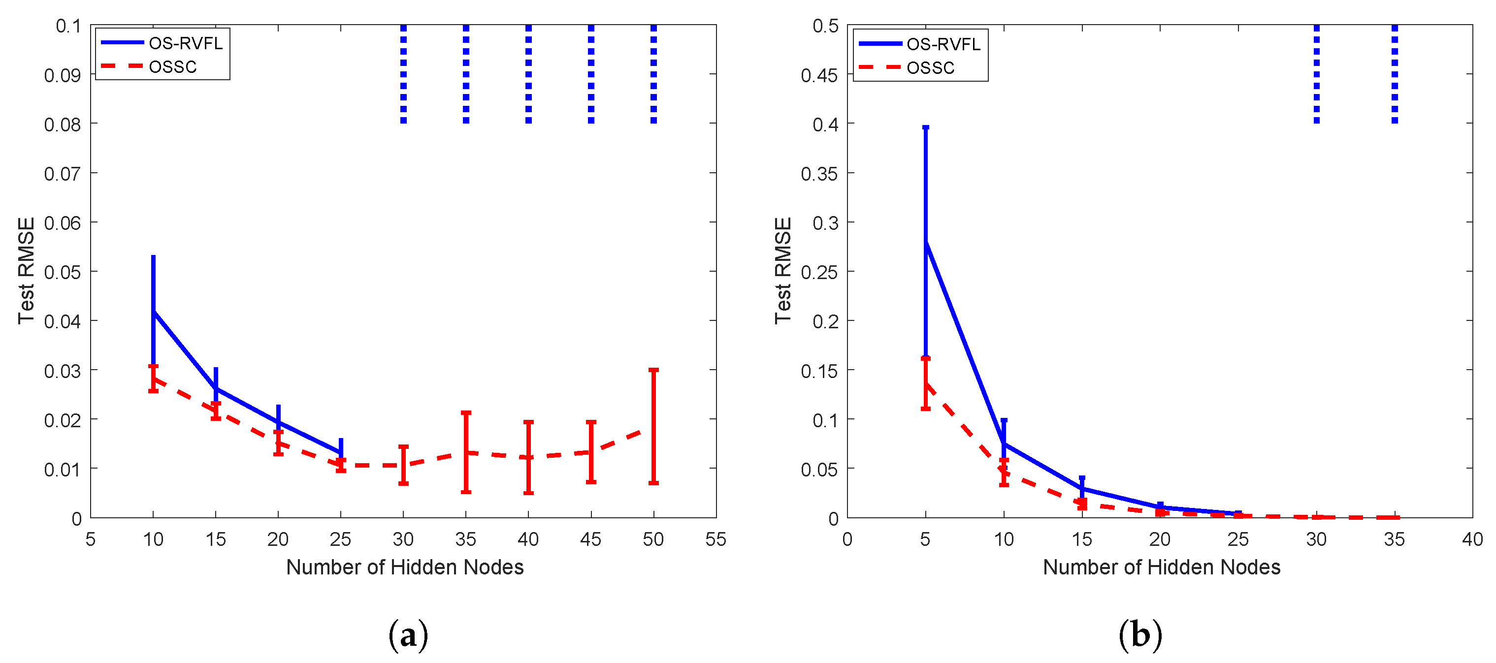
, it is clear that OSSC have obtained better test results than OS-RVFL in all the situations considered in the experiments. For example, when $N_0=300$, chunk size is set to 50, the resulting averaged RMSE of OS-RVFL is $0.0103$ while that of OSSC is $0.0076$, which means that OS-RVFL’s error is nearly 1.5 times larger than that of OSSC. To further uncover the potential advantages of OSSC over OS-RVFL, we fix the chunk size as 1, consider two settings of initial training samples, i.e., $N_0=100,50$, respectively, and try different setting of the number of hidden nodes (e.g., L) for both OSSC and OS-RVFL. As shown in Figure 4, it is interesting that OS-RVFL fails in certain cases, as marked as the blue dotted ellipses, while OSSC is feasible and effective in all the cases. Specifically, as can be seen in Figure 4a, when the number of hidden nodes of OS-RVFL is larger than 30, the resulted model significantly overfits the test samples, which in other words leads to a huge test error. This is why we have used the blue dotted ellipses to reflect this ‘abnormal’ phenomenon, in contrast to the stable and favorable performance of OSSC. Similar findings, for example when the number of hidden nodes exceeds 30, can also be found in Figure 4b. In addition, we see clearly in Figure 5 that the error curve of OS-RVFL is much worse than that of OSSC. Therefore, OSSC outperforms OS-RVFL in problem-solving for this kind of sequential learning task.

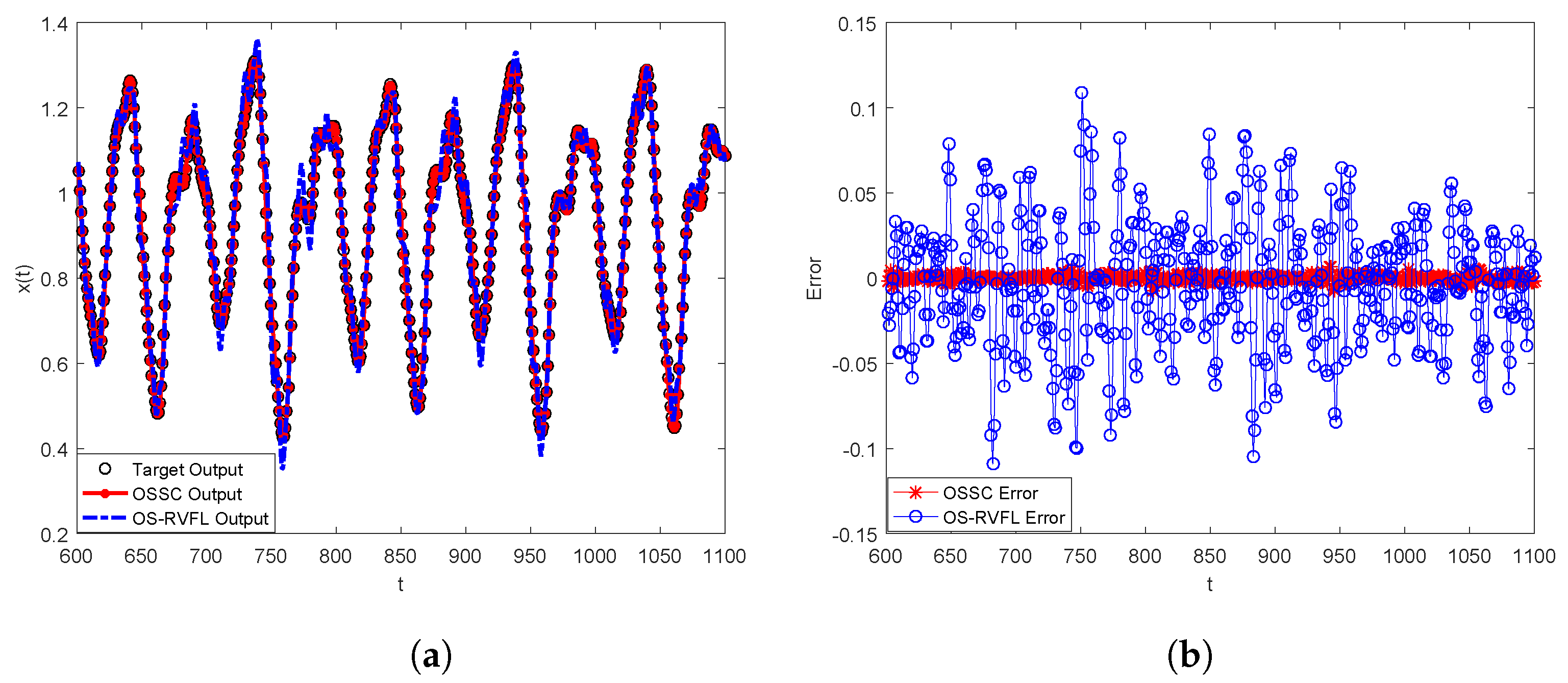
5.3. Mackey–Glass Time-Series Prediction

The third task we consider in our experimental study is the classic Mackey–Glass time-series prediction, which has been widely used in literature to test the performance of neural networks on nonlinear chaotic system modeling. The time series used in this part is derived from a time-delay differential system with the following form:

$$\frac{dy}{dt}=\frac{ay(t-\tau )}{1+y^n(t-\tau )}+by\left(t\right),$$

where $n=10$, $a=0.2$, $b=-0.1$, $\tau =17$, and the initial condition $y\left(0\right)=1.2$.

The aim of this experiment is to model the Mackey–Glass chaotic system using OSSC and OS-RVFL, respectively, and to predict the value $x(t+6)$ from $\left\{x\right(t),x(t-6),x(t-12),x(t-18\left)\right\}$. Five hundred data points with $t\in [101,600]$ are chosen as the training samples, and five hundred data points with $t\in [601,1100]$ are used as test samples to evaluate the performance of OSSC and OS-RVFL.

As shown in

Table 4. Test performance comparison for the Mackey–Glass time-series prediction task. MEAN and STD denote the average value and standard deviation of RMSE values.

${\mathit{N}}_0$ Values	Algorithms	Test Performance with Different Chunk Size (MEAN, STD)
		1 by 1	10 by 10	20 by 20	50 by 50
$N_0=50$	OS-RVFL	0.0038, 0.0017	0.0037, 0.0016	0.0038, 0.0017	0.0035, 0.0015
	OSSC	0.0018, 6.7672 × ${10}^{-4}$	0.0017, 6.3603 × ${10}^{-4}$	0.0017, 6.2183 × ${10}^{-4}$	0.0017, 5.8115 × ${10}^{-4}$
$N_0=100$	OS-RVFL	0.0012, 7.6733 × ${10}^{-4}$	0.0013, 8.8951 × ${10}^{-4}$	0.0013, 0.0015	0.0011, 6.5840 × ${10}^{-4}$
	OSSC	3.9257 × ${10}^{-4}$, 1.7408 × ${10}^{-4}$	3.6046 × ${10}^{-4}$, 1.7566 × ${10}^{-4}$	3.6421 × ${10}^{-4}$, 1.6275 × ${10}^{-4}$	3.6826 × ${10}^{-4}$, 1.8212 × ${10}^{-4}$
$N_0=150$	OS-RVFL	0.0012, 7.3932 × ${10}^{-4}$	0.0012, 7.0551 × ${10}^{-4}$	0.0012, 7.1992 × ${10}^{-4}$	0.0039, 0.0279
	OSSC	3.5359 × ${10}^{-4}$, 1.6470 × ${10}^{-4}$	3.5709 × ${10}^{-4}$, 1.8728 × ${10}^{-4}$	3.1413 × ${10}^{-4}$, 1.4894 × ${10}^{-4}$	3.4146 × ${10}^{-4}$, 1.9137 × ${10}^{-4}$

, OSSC outperforms OS-RVFL in all the cases. For example, when $N_0=150$, chunk size is 50, the averaged test RMSE of OSSC is 3.4146 × ${10}^{-4}$ while that of OS-RVFL is $0.0039$. Approximately, OS-RVFL’s error is 11 times larger than that of OSSC. Furthermore, as can be seen in Figure 6, similar to the findings found in Figure 2, Figure 3 and Figure 5, the error curves of OSSC reflect its better generalization capabilities than OS-RVFL. In summary, OSSC works more favorably than OS-RVFL in dealing with the Mackey–Glass time-series prediction problem, which further verifies the good potential of OSSC algorithm for (online) sequential learning. Furthermore, OSSC shows better stability over OS-RVFL, as demonstrated in Figure 7.

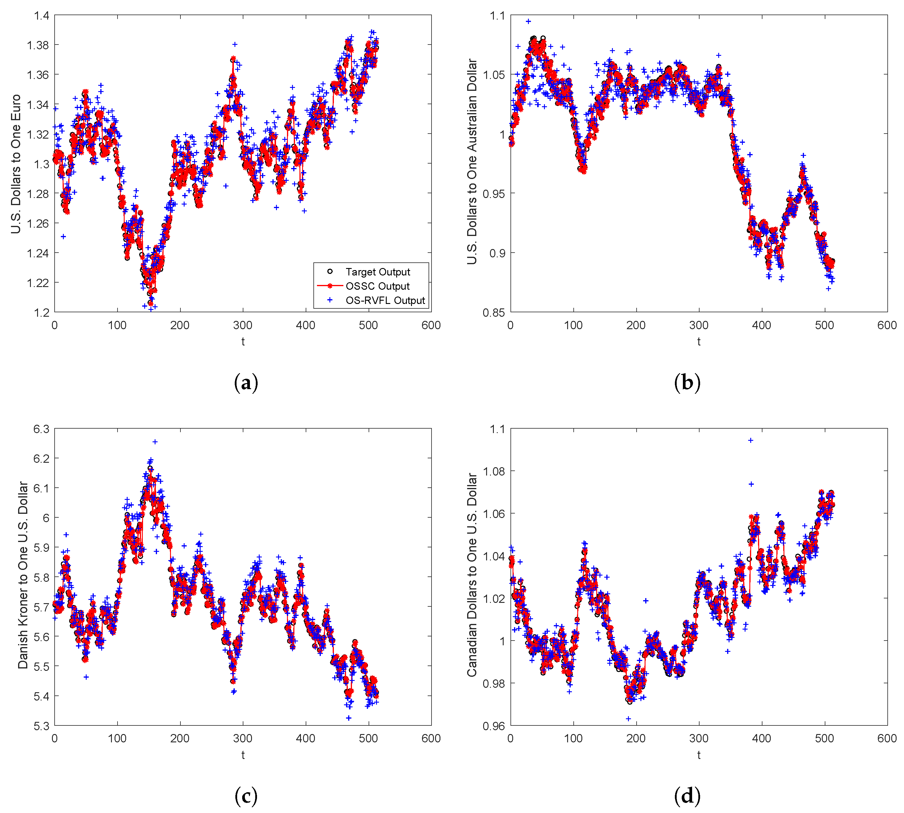
5.4. Application in Foreign Exchange Rate Forecasting

To further explore the effectiveness and advantages of OSSC for problem-solving in real-world applications, we compare OSSC and OS-RVFL with a real dataset for the foreign exchange rate forecasting task. In particular, we start with a detailed description of the data preparation process, then demonstrate the performance comparison based on extensive experimental results, followed by a robust analysis to investigate empirically the influence of the chunk size on the model’s performance. All the experimental results have verified the advantages of OSSC over OS-RVFL, delineated as follows.

5.4.1. Data Preparation

The datasets utilized in this part are all downloaded from the official website of American Federal Reserve Bank (https://fred.stlouisfed.org/fred-addin/, accessed on 1 March 2022), in which 2542 exchange rates from 1 January 2004 to 27 September 2013 are chosen to verify the effectiveness of OSSC and OS-RVFL. In particular, four types of foreign exchange, including US Dollar/Euro, U.S. Dollar/Australia Dollar, Danish Kroner/U.S. Dollar, and Canadian Dollar/U.S. Dollar. The missing observations in the above period are removed from the chosen data. Finally, we can obtain 2453 observations for each data set. The time window size for the following 1-day-ahead forecasting is chosen as 5. Hence, there are 2448 samples for each data set. Among them, based on the partition of time-series, 1836 samples, 306 samples, and 306 samples are utilized as the training set, validation set, and test set, respectively.

5.4.2. Performance Illustration

In

Table 5. Test performance comparison for the real-world foreign exchange rate forecasting task. MEAN and STD denote the average value and standard deviation of RMSE values. Abbreviations used in this table: U/E: U.S. Dollar/Euro, U/A: U.S. Dollar/Australia Dollar, D/U: Danish Kroner/U.S. Dollar, C/U: Canadian Dollar/U.S. Dollar.

Cases	Algorithms	Test Performance with Different Chunk Size (MEAN, STD)
		1 by 1	10 by 10	20 by 20	50 by 50
U/E	OS-RVFL	0.0146, 3.46 × ${10}^{-4}$	0.0147, 6.42 × ${10}^{-4}$	0.0146, 4.18 × ${10}^{-4}$	0.0147, 7.56 × ${10}^{-4}$
	OSSC	0.0068, 2.43 × ${10}^{-5}$	0.0068, 2.46 × ${10}^{-5}$	0.0068, 5.10 × ${10}^{-5}$	0.0068, 2.49 × ${10}^{-5}$
U/A	OS-RVFL	0.0210, 5.67 × ${10}^{-3}$	0.0191, 4.36 × ${10}^{-3}$	0.0182, 5.78 × ${10}^{-3}$	0.0175, 3.56 × ${10}^{-3}$
	OSSC	0.0066, 4.99 × ${10}^{-4}$	0.0067, 5.60 × ${10}^{-4}$	0.0067, 5.50 × ${10}^{-4}$	0.0067, 4.06 × ${10}^{-4}$
D/U	OS-RVFL	0.1017, 8.51 × ${10}^{-2}$	0.0921, 4.51 × ${10}^{-2}$	0.0835, 3.51 × ${10}^{-2}$	0.0717, 4.11 $\times {10}^{-2}$
	OSSC	0.0310, 1.30 × ${10}^{-3}$	0.0307, 7.85 × ${10}^{-4}$	0.0311, 1.40 × ${10}^{-3}$	0.0307, 6.52 × ${10}^{-4}$
C/U	OS-RVFL	0.0126, 6.73 × ${10}^{-3}$	0.0097, 2.73 × ${10}^{-3}$	0.0088, 7.73 × ${10}^{-4}$	0.0084, 2.42 $\times {10}^{-4}$
	OSSC	0.0041, 1.73 × ${10}^{-5}$	0.0041, 1.78 × ${10}^{-5}$	0.0041, 1.74 × ${10}^{-5}$	0.0041, 2.01 × ${10}^{-5}$

, it is clear that OSSC outperforms OS-RVFL on all the four datasets with different chunk size settings. For example, for the case of U.S. Dollar/Euro, the averaged RMSE values obtained by OS-RVFL are generally two times larger than that of OSSC in all the situations. As for the other cases, such as U.S. Dollar/Australia Dollar, Danish Kroner/U.S. Dollar, Canadian Dollar/U.S. Dollar, the averaged RMSE values resulted by OS-RVFL are nearly four times larger than that of OSSC in all the situations. To better indicate the performance comparison, in Figure 8, we plot the target outputs, OSSC outputs, OS-RVFL outputs, respectively, for all the four datasets. As can be seen clearly, OSSC achieves better prediction than OS-RVFL for all the four cases, which is consistent with the test RMSE records summarized in Table 5.

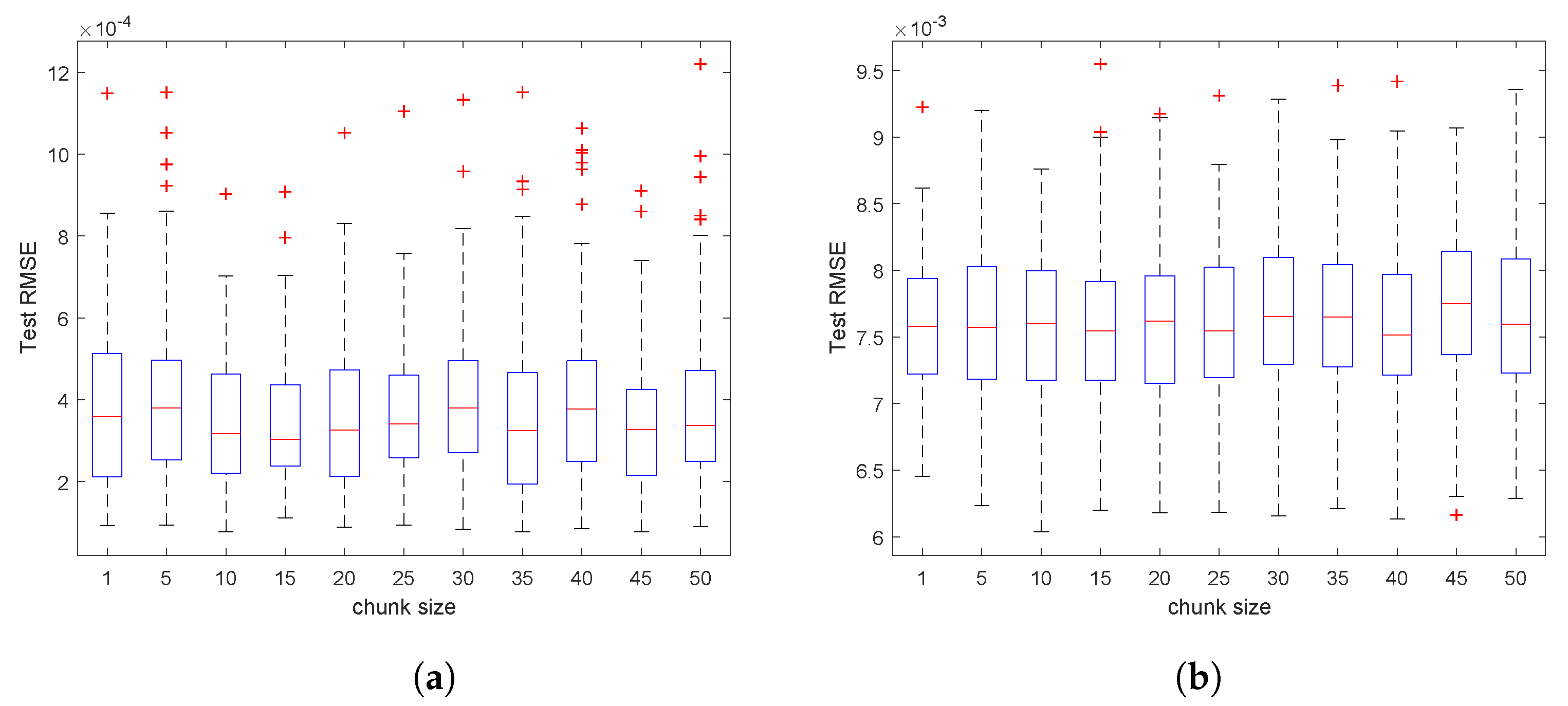
5.4.3. Robust Analysis

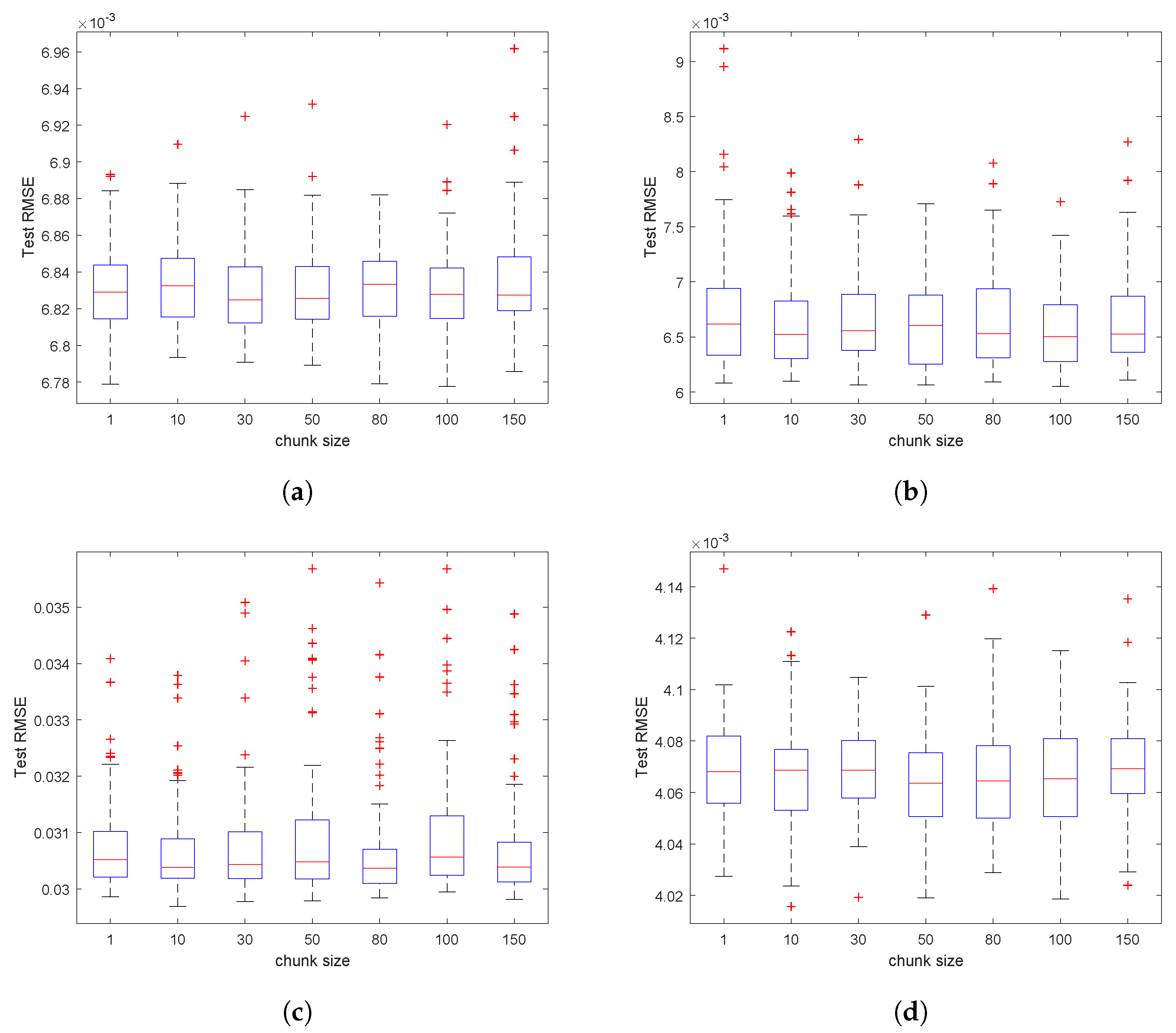
To further demonstrate the merits of OSSC for the problem-solving of foreign exchange rate forecasting, in this part, we investigate empirically the impact of the chunk size on the OSSC’s test performance. In particular, for each dataset, we run 50 trials independently for each chunk size settings (=$1,10,30,50,80,100,150$, respectively), then draw the boxplot for each case, of which the central mark indicates the median, and the bottom and top edges of the box indicate the 25th and 75th percentiles, respectively, and the outliers are plotted individually using the ‘+’ marker symbol, see Figure 9. It shows clearly that OSSC works stably for all the settings of different chunk size, which to some extent offers some guidance for users when employing OSSC in similar tasks.

Overall, based on all the presented experimental results and discussion in this section, we can draw a convincing conclusion that OSSC can be used as an effective online sequential learning algorithm for neural networks, and it has good potential to contribute to favorable learner models with sufficient capability for streaming data modeling tasks, such as nonlinear dynamic system modeling, time-series prediction, foreign exchange rate forecasting, and so on.

6. Conclusions

This paper has extended the previously-proposed stochastic configuration (SC) algorithm into an online sequential version that can effectively work on sequentially given training observations. The recursive least square (RLS) approach is used in formulating our OSSC algorithm. The primary motivation behind our work is that the commonly-used (offline) RVFL-based randomized algorithm, i.e., randomly assigning the input weights and biases and only optimizing the output weights, may possibly fail in bringing a universal approximator due to an inappropriate setting of random parameters, which consequently incurs potential danger for the corresponding online sequential extension (OS-RVFL). The merits of SC have been retained in the online learning process as the initial base model (with the first available data) is constructed by SC, instead of being trained by the RVFL-based randomized algorithm. Extensive experiments have validated that our proposed OSSC algorithm outperforms OS-RVFL on both synthetic datasets (1D function approximation, nonlinear dynamic system modeling, time-series prediction) and real-world application (foreign exchange rate forecasting). Extensions of the present algorithm to a more advanced version that can self-organize the neural network structure via growing and/or pruning schemes, or a robust version that works favorably on data contaminated with varying degrees of outliers, are being expected. In addition, based on our idea presented in this work, it is interesting to study the online sequential learning algorithm for graph neural networks (with random weights) that have received careful attention in recent years [32,33,34].