Multi-Scenario Simulation of Land Use Change and Ecosystem Service Value in the Middle Reaches of Yangtze River Urban Agglomeration

Abstract

The evolution of regional land use is a complex process under the combined effect of multiple factors, and it is important to understand this evolution process, as well as its characteristics and future trends, through land use change models in order to achieve scientific use of land space and optimize the regional development pattern. In this study, the PLUS model is used to simulate the land use in 2035 for the natural development scenario, the urban expansion scenario and the ecological protection scenario using the middle reaches of Yangtze River urban agglomeration (MRYRUA) as the study area, and then to calculate the ecosystem service values (ESV) and analyze the contribution of each driver to each land type and the spatial autocorrelation of the ESV at the grid scale. The results show that (1) the land use changes in the study area from 2015 to 2020 are mainly: the rapid expansion of construction land with an increase of 200,221 hm² and an increase in arable land, specifically 85,982 hm², and a decrease in all other land types. (2) The ESV of the study area was CNY 3,837,282 million and CNY 3,774,162 million from 2015 to 2020, respectively, with an general decreasing trend. (3) Three scenarios are simulated for the study area in 2035, and the ESVs under the natural development scenario, urban expansion scenario and ecological conservation scenario are CNY 3,618,062 million, CNY 3,609,707 million and CNY 3,625,662 million, respectively, which are all lower than those in 2020. (4) The global autocorrelation indices for 2020 and the three scenarios are 0.7126, 0.7104, 0.7144 and 0.7104, respectively, which are significantly positive. The simulation of MRYRUA land use and the comparative analysis of ESV provide some help in the strategic optimization of the spatial distribution pattern of land use in large regional urban agglomerations.

1. Introduction

Ecosystem services (ES) refer to all benefits that humans obtain from ecosystems, and the assessment of their value is closely related to changes in land use. Ecosystem service values (ESV) serve as an important basis for ecological protection, ecological function zoning, environmental-economic accounting and ecological compensation decisions [1,2]. Currently, human activities are leading to huge changes in land use, with a large amount of natural ecological land evolving into man-made land, limiting the performance of various ecosystem services and functions and affecting the assessment of ESV [3]. Land use practices that are inappropriate for regional development can affect sustainable regional development and damage the ecological environment [4]. As a key region for promoting the rise of the central region, deepening reform and opening up and promoting new urbanization, the Yangtze River urban agglomeration (MRYRUA) inevitably features intensive human activities, which have transformed a large area of ecological land into urban construction land. Such large-scale land development and utilization will cause serious damage to the local ecological environment and hinder the realization of balanced and sustainable regional development [5,6]. In this context, modeling land use changes and their impacts on ESV in the MRYRUA under various scenarios can provide some guidance for future balanced sustainable development of the region [7].

Thus far, scholars in China and abroad have conducted a large number of studies on the relationship between land use and ESV. Since Costanza proposed a method for evaluating the value of ecological services in Nature in 1997, scholars around the world have gradually been paying attention to ESV. Based on Costanza’s work, Xie et al. [8,9] conducted a questionnaire survey of 200 professionals in China with ecological backgrounds and proposed a new equivalence factor scale applicable to China. Subsequently, numerous scholars have conducted a large number of studies on ESV, from theoretical studies on definition and classification [10,11,12] to empirical studies, such as value assessment [13,14,15]. As research progressed, scholars gradually realized that existing studies on ESV were mostly focused on the analysis of historical land use data, while predictions of future land use under multiple scenarios were inadequate. Accordingly, scholars began to introduce predictive models and apply them to the prediction of future land use conditions. In particular, cellular automata (CA) [16,17,18] systems have been used as the basis for the construction of prediction models, and through continuous development, the CLUE-S model [19,20,21], SLEUTH model [22,23,24], system dynamics (SD) [25,26,27] and FLUS (future land use simulation) models have been designed [28,29,30]. However, these models cannot handle the evolution of land use over large regions and multiple land types. The PLUS (patch-generating land use simulation) model [31,32,33] is an emerging land use prediction model that can simulate land use changes at large scales and multiple land classes more accurately. It can also analyze the driving factors and the extent of their contribution. Therefore, it offers significant advantages in conducting land use simulation.

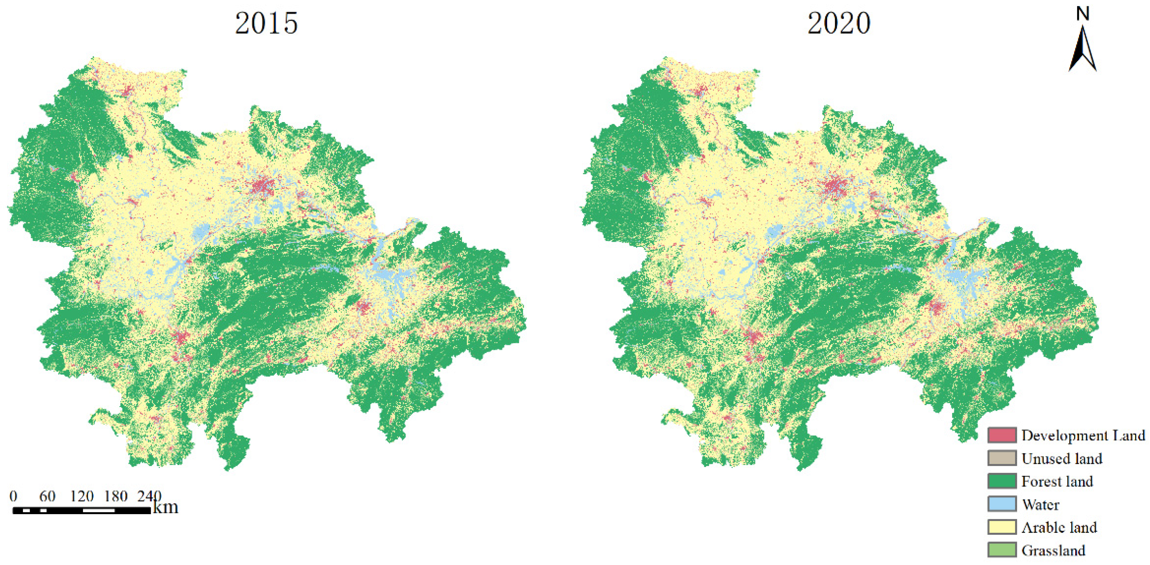
The rapid development of the MRYRUA will inevitably exert great pressure on the local ecological environment, thus affecting the ESV, and damaged ecological environments may not be able to meet the needs of urban agglomeration development. Therefore, this paper decodes the land use data of the middle reaches of Yangtze River urban agglomeration in 2010, 2015 and 2020 by remote sensing technology, predicts the land use in 2020 by using the PLUS model and the data of 2010 and 2015, compares the actual situation in 2020 to verify the accuracy of the model and then predicts the land use of the natural development scenario, urban expansion scenario and ecological protection scenario in 2035 by using the data of 2015 and 2020. The ESV under each scenario was then calculated using the method of equivalent factor, and the spatial autocorrelation of ESV was analyzed. The findings will contribute toward establishing a foundation for the improvement of the spatial pattern of land use at the national level, as well as ecological protection policies of the MRYRUA.

2. Materials and Methods

2.1. Study Area

The MRYRUA, otherwise called the “middle triangle”, is located at 26°03′–32°38′ N, 110°45′–118°21′ E (Figure 1), and includes the Wuhan City Cluster, Changzhutan City Cluster and Poyang Lake City Cluster. The specific scope includes 13 cities, such as Wuhan, Huangshi, and Xiaogan, in Hubei Province; 8 cities, such as Changsha and Zhuzhou, in Hunan Province; 9 cities, such as Nanchang, Jiujiang and Jingdezhen, in Jiangxi Province; and some counties in Ji’an City, totaling 31 cities. The MRYRUA has a subtropical monsoon climate, with an average annual precipitation of approximately 800–1943 mm and an altitude of 20–3105 m above sea level. The land area of the MRYRUA is 317,000 km², accounting for 3.3% of the total land area, with a total population of 125 million people and a regional GDP of CNY 7.90 trillion. It is a significant member of the Yangtze River Economic Belt and a vital region for executing the methodology of advancing the ascent of the focal locale, extending change and, on all fronts, opening up and advancing new-type urbanization. It plays a significant role in the regional development of China.

2.2. Data Sources

The types of data used in this study include administrative boundary, land use, human activity, DEM topographic, climate and restricted areas. The specific sources of these data are as follows (

Table 1. Data sources.

Data Type		Data Name	Data Source
Basic data	Administrative boundaries	Administrative Boundary of the Middle Yangtze River City Cluster	National Center for Basic Geographic Information
	Land use	Land use data of the MRYRUA for 2010, 2015 and 2020	A research paper entitled “30 m annual land cover and its dynamics in China from 1990 to 2019”, co-authored by Professors Yang Jie and Huang Xin of Wuhan University
Driving factors	Human activities	Population Density	https://www.worldpop.org/, accessed on 25 June 2020
		GDP	Resource and Environmental Science and Data Centre, Chinese Academy of Sciences
		Distance to railway	National Center for Basic Geographic Information
		Distance to road	National Center for Basic Geographic Information
		Distance to river	National Center for Basic Geographic Information
	Topography	DEM	Geospatial Data Cloud
		Slope	Geospatial Data Cloud
		Slope direction	Geospatial Data Cloud
	Climate	Average annual temperature	https://crudata.uea.ac.uk/cru/data/hrg/, accessed on 25 June 2020
		Average annual precipitation	https://crudata.uea.ac.uk/cru/data/hrg/, accessed on 25 June 2020
Restricted areas	Restricted area vector data	Nature reserves	China Nature Reserve Specimen Resource Sharing Platform
		Surface water system	Chinese Academy of Sciences Resource and Environmental Science and Data Centre

): (1) The shapefile of administrative boundaries of the MRYRUA were acquired from the National Center for Basic Geographic Information. (2) Land use vector data for 2010, 2015 and 2020 were obtained from a paper [34] co-authored by Professors Yang Jie and Huang Xin of Wuhan University, and the equivalent factor table of Xie Gaodi et al. [8] was referred to reclassify land use into six types (arable land, forest land, grassland, water, development land and unused land). (3) Population density vector data of China were obtained from the WorldPop web portal (https://www.worldpop.org/, accessed on 25 June 2022) and GDP vector data of China were obtained from the Resource and Environment Science and Data Centre of the Chinese Academy of Sciences. The obtained data were extracted by masking, according to the administrative boundary data, to obtain the population density and GDP data of the study area. (4) The shapefile of road and river data were obtained from the National Center for Basic Geographic Information, utilizing the Euclidean distance tool to acquire the distance to railways, roads and rivers. (5) The Geospatial Data Cloud provides the DEM vector data, and the slope and slope direction data were acquired by handling the DEM data with the slope and slope direction tools in the 3D Analyst tool. (6) NetCDF data for climate were obtained from the website of the Climate Research Unit (https://crudata.uea.ac.uk/cru/data/hrg/, accessed on 25 June 2020), including average annual temperature and average annual precipitation, and they were processed by image element statistics and inverse distance weighting method interpolation analysis. (7) Restricted area data include nature reserve vector data and surface water system vector data. Land use was reclassified according to the restricted area data; restricted areas were reclassified as 0, and the remaining unrestricted areas within the study area were reclassified as 1.

2.3. Research Methods

2.3.1. Ecosystem Service Values

In this study, the ESV per unit area in the MRYRUA in 2015 and 2020 was estimated using the ecosystem service equivalent table developed by Xie Gaodi et al. [8], and its change characteristics were analyzed. The calculation method is shown in Equation (1).

$$ESV={\displaystyle \sum }{A}_k\times V{C}_k$$

(1)

where ESV is the ecosystem service value, CNY; A_k is the area of the kth land use type in the study area, hm²; and VC_k is the ESV coefficient, that is, the ESV per unit area of the kth land use type, CNY /hm².

Considering that the monetary worth of production services per unit of arable land is seven times higher than the economic value of natural ecosystems without human input [35], this study applied Equation (2) to obtain the equivalent ESV of CNY 2198.17/hm² based on the production, planted area and unit price of major food crops in Hunan, Hubei and Jiangxi provinces in 2020. We then constructed an ecosystem service value coefficient table (

Table 2. List of ESV coefficients (CNY/hm²).

First Classification	Second Classification	Arable Land	Forest Land	Grassland	Water	Development LAND	Unused Land	Total
Supply Services	Food production	4858	2220	1539	1759	0	22	10,397
	Raw material production	1077	5100	2264	506	0	66	9013
	Water supply	−5737	2638	1253	22,971	0	44	21,168
Regulation Services	Gas regulation	3913	16,772	7957	2088	0	286	31,016
	Climate regulation	2044	50,184	21,037	6221	0	220	79,706
	Purification of the environment	594	14,706	6946	12,552	0	901	35,698
	Hydrological regulation	6573	32,841	15,409	240,414	0	528	29,574
Support Services	Soil conservation	2286	20,421	9694	2044	0	330	34,775
	Maintenance of nutrient cycles	681	1561	747	154	0	22	3165
	Biodiversity	747	18,597	8815	5627	0	308	34,094
Cultural Services	Aesthetic landscape	330	8155	3891	4352	0	132	16,860
Total		17,366	173,194	79,552	298,688	0	57,167	2858

).

$$V{C}_k=\frac{1}{7}{\displaystyle \sum }_{i=1}^n\frac{m_i{p}_i{q}_i}{M}\left(i=1,2,\dots ,n\right)$$

(2)

where i is the main food type; m_i is the sown area of crop i, hm²; p_i is the national average price of crop i, CNY/kg; q_i is the unit yield of crop i, kg/hm²; and M is the total area of the main food crops in the study area, hm².

2.3.2. PLUS Model

• Introduction to the model

This study uses the patch-generating land use simulation (PLUS) proposed by Liang et al. [31]. The model applies the Land Expansion Analysis Strategy (LEAS), a CA based on Multiple Random Seeds (CARS) coupled with multiobjective programming, and the simulation results can better support planning policies to achieve sustainable development.

The model first applies the Land Expansion Analysis Strategy (LEAS) to uncover the causal factors of each type of land use change. The strategy extracts the parts of each type of land use expansion between the two periods of land use change. In addition, sampling from the increased part is conducted using the random forest algorithm to mine the factors of each type of land use expansion and drivers individually, in order to obtain the development probability of each type of land use and the contribution of drivers to the expansion of each type of land use in that time period. Then, using CARS, combined with stochastic seed generation and a threshold-decreasing mechanism, allows the model to automatically generate dynamically simulated patches within the constraints of development probabilities. This new multiclass seed growth mechanism allows for better simulation of multiclass land use patch-level changes. The final multiobjective programming refers to the identification of sustainable land use structures to support decision making in the study area through the objective optimization function, constraints and parameters proposed by Wang et al. [36].

2.

Scenario setting

In this study, three scenarios of natural development, urban expansion and ecological protection were set for future land use development in the MRYRUA, and a land development law and conversion cost matrix was developed for each scenario.

3.

Simulation process

First, the data of 10 driving factors and the land use data of 2010, 2015 and 2020 in the study area were preprocessed to pair the row numbers of each data and to unify the coordinate system. Then, the format of the above data was converted in the PLUS model, and the land use data of 2015 and 2020 were entered. The Extract Land Expansion module was then used to extract the land expansion of each type of land between 2010 and 2015. Subsequently, by entering each driving factor and the land expansion data obtained in the previous step into the LEAS module, we were able to obtain the development probability of each land type for the transfer to other land types in the time span of 2020–2035, as well as the contribution of each driving factor to the development probability. Then, development probability data, land demand data which was calculated by Markov chain and adjusted, and restricted area data were input. The transfer matrix and neighborhood weights of each scenario were set under the CARS module, and the simulated land use vector distribution map of the study area in 2035 was obtained. Finally, the ESV of the study area was calculated using the land use vector distribution map obtained from the simulation. The workflow is shown in Figure 2.

4.

Selection of driving factors

Considering the actual situation of the MRYRUA and the availability of data, 10 driving factors (population density, GDP, distance to railroad, distance to road, distance to river, DEM, slope, slope direction, average annual temperature and average annual precipitation) were selected from the three aspects of human activities, topography and climate.

5.

Restricted area setting

In this study, nature reserves and surface water systems were set as restricted areas in the ecological conservation scenario through ArcGIS 10.2, with 0 indicating restricted areas and 1 indicating convertible areas. Restricted areas were set in the ecological conservation scenario, but not in the natural development and urban expansion scenarios.

6.

Land demand

The land demand in the MRYRUA in 2035 under the natural development scenario was calculated based on the land use data in 2015 and 2020, with the help of Markov chains. The other scenarios were adjusted for land demand with reference to the relevant literature [37,38]. With reference to the natural development scenario, the likelihood of arable land, forest land, grassland, water and unused land converting to development land by 20% is increased under the urban expansion scenario, whereas the likelihood of development land converting to other land by 30% is decreased. Under the ecological conservation scenario, the likelihood of arable land and forest land converting to development land by 30% is decreased, the likelihood of grassland and water converting to development land by 20% is decreased, the likelihood of unused land converting to development land by 10% is decreased and the likelihood of development land converting to forest land by 10% is increased.

7.

Cost transfer matrix

Referring to many relevant pieces of literature [39,40,41], the cost matrix of conversion for the three scenarios is shown in

Table 3. Conversion cost matrix.

	Natural Development Scenarios						Urban Expansion Scenarios						Ecological Conservation Scenarios
	I	II	III	IV	V	VI	I	II	III	IV	V	VI	I	II	III	IV	V	VI
I	1	1	1	1	1	1	1	0	0	0	1	1	1	1	1	1	1	1
II	1	1	1	1	1	1	1	1	0	0	1	1	0	1	0	0	0	0
III	1	1	1	1	1	1	1	0	1	0	1	1	0	1	1	1	0	0
IV	1	1	1	1	1	1	1	0	0	1	1	1	0	0	0	1	0	0
V	0	0	0	0	1	0	0	0	0	0	1	0	0	0	0	0	1	0
VI	1	1	1	1	1	1	1	1	1	1	1	1	1	1	1	1	1	1

, where I to VI denote arable land, forest land, grassland, water, development land and unused land in that order, with 0 representing no conversion and 1 representing conversion.

8.

Neighborhood weight parameter setting

The neighborhood weight parameter is a representation of the expansion intensity of different types of land, which reflects the expansion capacity of different types of land driven by various driving factors. The parameter ranges from 0 to 1, with higher values indicating greater neighborhood influence. This study, therefore, used land use data from 2015 and 2020 and applied Equation (3) to calculate the neighborhood weights. In addition, using this formula, the neighborhood weight parameter of the unused land is calculated as 0, since any land has the ability to expand, the parameter is made to be 0.0001. The specific neighborhood parameters are shown in

Table 4. Neighborhood weight parameters.

Land Use Type	Arable Land	Forest Land	Grassland	Water	Development Land	Unused Land
Neighborhood weights	0.43	0.77	0.03	0.62	1	0.0001

.

$$W_i=\frac{X_i-X_{min}}{X_{max}-X_{min}}$$

(3)

where W_i is the neighborhood weight of the ith land use type, X_i is the number of land use pixels of the ith land use type, X_min is the smallest land use pixel of all land use types and X_max is the largest land use pixel of all land use types.

9.

Accuracy check

The land use data of 2010 and 2015 were used to simulate the land use in 2020, and then, the simulated land use in 2020 was integrated with the actual land use data in 2020. The accuracy of both simulations was verified in terms of the Kappa coefficient and the Fom coefficient. The Kappa value was 0.91, indicating an overall accuracy of 95.28%, and the Fom value was 0.47. These values demonstrate that the model has high simulation accuracy, and is suitable for simulating land use changes in the MRYRUA in 2035.

2.3.3. Spatial Autocorrelation

Spatial autocorrelation analysis is an analytical method for assessing whether the distribution of some variables within a study area is agglomerative. It comprises global and local spatial autocorrelation analysis, and mainly employs Moran’s I for analysis and measurement.

10.

Global spatial autocorrelation

In assessing the existence of spatial autocorrelation and spatial variability in the study area, global spatial autocorrelation is usually used, and the specific methods mainly include the Moran’s I index [42,43], Geary index [44] and Getis index [45]. In this study, Moran’s I was primarily used, and the calculation method which was applied is as follows.

$$Mora{n}^{’}s I=\frac{n{{\displaystyle \sum }}_{i=1}^n{{\displaystyle \sum }}_{j\ne 1}^n{w}_{ij}\left(x_i-\overline{x}\right)\left(x_j-\overline{x}\right)}{\left({{\displaystyle \sum }}_{i=1}^n{{\displaystyle \sum }}_{j=1}^n{w}_{ij}\right){{\displaystyle \sum }}_{i-1}^n{\left(x_i-\overline{x}\right)}^2}$$

(4)

where n is the number of spatial cells; x_i and x_j represent the observations of the variable x at the ith and jth spatial cell, respectively; $\overline{x}$ is the mean value of x and w_ij is the spatial weight matrix. A value of 1 means x_i and x_j are adjacent, and a value of 0 means they are not adjacent.

11.

Local spatial autocorrelation

Global spatial autocorrelation can only be used to assess the spatial correlation and spatial variability of the whole region, and cannot reflect the spatial autocorrelation between local regions. Nevertheless, this shortcoming can be overcome using Moran’s I_i (LISA) [46], which is expressed as follows.

$$Mora{n}^{’}s Ii=\frac{\left(x_i-\overline{x}\right)}{m_0}{\displaystyle \sum }_j{w}_{ij}\left(x_i-\overline{x}\right)$$

(5)

$$m_0=\frac{{{\displaystyle \sum }}_i{\left(x_i-\overline{x}\right)}^2}{n}$$

(6)

where a value of Moran’s I_i greater than 0 indicates a spatial aggregation of high–high or low–low values of spatial units, and a value of Moran’s I_i less than 0 indicates a spatial aggregation of high–low or low–high values of spatial units.

3. Results

3.1. Spatial and Temporal Variability in ESV

3.1.1. Characteristics of Land Use Change in the MRYRUA during 2015–2020

The land use types of the MRYRUA were mainly arable land and forest land between 2015 and 2020 (Figure 3). Under the guidance of the Implementation Plan for the 14th Five-Year Plan for the Development of the MRYRUA, the urbanization development of the MRYRUA has been taken as the primary task, with the aim of achieving an early urbanization rate of 67% of the resident population. This effort reinforced the high-quality development and use control of arable land, resulting in an overall upward trend in development land, and the overall trend of arable land has been on the rise. In addition, forest land, grassland, and water all exhibited a decreasing trend, indicating that the development of economic urbanization has, to a certain extent, led to the occupation of ecological land by man-made surfaces, resulting in the destruction and degradation of ecosystems.

Specifically, development land experienced the greatest change in the area, changing from 1,362,741 hm² in 2015 to 1,562,962 hm² in 2020, with an increase of 200,221 hm² (

Table 5. Land use area in 2015 and 2020.

Land Use Type		Arable Land	Forest Land	Grassland	Water	Development Land	Unused Land
2015	Area (hm2)	17,031,683	1,719,0558	15,472	1,884,845	1,362,741	2161
	proportion (%)	45.433	45.857	0.041	5.028	3.635	0.006
2020	area (hm2)	17,117,665	17,035,986	9168	1,759,830	1,562,962	1849
	proportion (%)	45.662	45.444	0.024	4.694	4.169	0.005
Amount of area change 2015–2020 (hm2)		85,982	−154,572	−6304	−125,015	200,221	−312
Rate of change in area 2015–2020 (%)		0.505	−0.899	−40.744	−6.633	14.693	−14.437

). The area of arable land, which is the main component of the study area, changed from 17,031,683 hm² in 2015 to 17,117,665 hm² in 2020, with an increase of 85,982 hm². Forest land, another major component land type in the study area, showed an overall decreasing trend, from 17,905,058 hm² to 17,035,986 hm². Grassland was the least occupied land type in the study area except for unused land, changing from 15,472 hm² to 9168 hm² during the study period, with a decrease of 6304 hm². The water area as a whole showed a decreasing trend, specifically from 1,884,845 hm² to 1,759,830 hm². The area of unused land, which occupies the smallest proportion in the study area, changed from 15,472 hm² in 2015 to 9168 hm² in 2020, with a decrease of 6304 hm².

3.1.2. Characteristics of ESV Changes during 2015–2020

The ESV of the MRYRUA exhibited a downward trend from CNY 3,837,282 million in 2015 to CNY 3,774,162 million in 2020, a cumulative decrease of CNY 63,121 million (

Table 6. ESV for 2015 and 2020.

Land Use Type		Arable Land	Forest Land	Grass Land	Water	Development Land	Unused Land
2015	ESV (CNY 1 million)	295,765	2,977,301	1231	562,980	0	6
	Proportion (%)	7.72	77.94	0.05	14.28	0.00	0.00
2020	ESV (CNY 1 million)	297,258	2,950,530	729	525,639	0	5
	Proportion (%)	7.88	78.18	0.02	13.93	0.00	0.00
Amount of ESV change (CNY 1 million)		1493	−26,771	−501	−37,341	0	−1
Rate of change in ESV (%)		−2.37	42.41	0.79	59.16	0.00	0.00

). Among the various land use types in the study area, forest land had the largest contribution to ESV, followed by water and arable land, with all three contributing to 99.9% of the ESV. Therefore, almost all of the ESV in the MRYRUA is attributable to forest land, water and arable land. In addition, development land has an ESV of 0 because its ESV coefficient is 0. According to the change in land use, only areas of development land and arable land showed an increasing trend, as development land is considered not to contribute to ESV. The ESV of only arable land showed an increasing trend over the study period, increasing from CNY 295,765 million in 2015 to CNY 297,258 million in 2020, a total increase of CNY 1,493,121 million. The ESV of the other four land use types showed a decreasing trend. Specifically, the ESV of forest land changed from CNY 2,977,301 million to CNY 2,950,530 million (a decrease of CNY 2,6771 million), but the ESV of forest land increased as a percentage of all land types, which may be because the decrease in the ESV of forest land was smaller than the overall decrease in ESV. Among all land use types, water showed the largest change in ESV, decreasing from CNY 562,980 million to CNY 525,639 million (a decrease of CNY 37,341 million), with the ESV change accounting for 59.16% of all ESV changes. In addition, the ESV of grassland and unused land both showed a decreasing trend, but because of their relatively small size, their ESV changes were also smaller, at CNY 502 million and CNY 0.89 million, respectively.

ES can be classified into four categories: provisioning services, regulating services, supporting services and cultural services, which can be further divided into 11 sub-categories, including food production and raw material production. In terms of the four broad categories, the largest contribution to ESV was from regulation services, which decreased from CNY 2,585,136 million to CNY 2,635,578 million, followed by support services, which decreased from CNY 775,883 million to CNY 768,830 million. Next is supply services, which decreased from CNY 222,191 million to CNY 217,482 million. The smallest change was from cultural services, which decreased from CNY 154,073 million to CNY 152,272 million during the study period. In terms of the 11 sub-categories, individual services contributing more than 10% were hydrological regulation, climate regulation and soil conservation, which collectively contributed more than 63%. In terms of changes in the function of each service (

Table 7. ESV for each individual service in 2015 and 2020.

First Classification	Second Classification	2015		2020
		ESV/ CNY 1 Million	Proportion/%	ESV/CNY 1 Million	Proportion/%
Supply Services	Food production	124,243	3.24	124,088	3.29
	Raw material production	107,001	2.79	106,228	2.81
	Water supply	−9053	−0.24	−12,834	−0.34
Regulation Services	Gas regulation	359,021	9.36	356,454	9.44
	Climate regulation	909,565	23.70	901,073	23.87
	Purification of the environment	286,676	7.47	282,841	7.49
	Hydrological regulation	1,129,874	29.44	1,095,210	29.02
Support Services	Soil conservation	393,989	10.27	390,712	10.35
	Maintenance of nutrient cycles	38,737	1.01	38,530	1.02
	Biodiversity	343,158	8.94	339,588	9.00
Cultural Services	Aesthetic landscape	154,073	4.02	152,272	4.03
Total		3,837,282	100.00	3,774,162	100.00

), the value of each service decreased during the study period, with hydrological regulation, climate regulation and environmental purification, all of which are regulation services, showing the largest changes. Among them, the values of the hydrological regulation function and environmental purification function were mainly influenced by water and forest land, and the value of the climate regulation function was mainly influenced by forest land and grassland. Accordingly, in the future economic development of the MRYRUA, environmental protection should be enhanced, land use should be rationalized and the protection of ecological land should be strengthened in order to advance the transformation from high-speed development to high-quality development in the MRYRUA.

Regarding the spatial distribution (Figure 4), the distribution of ESVs in the MRYRUA is mainly characterized by a decrease from the periphery to the center, followed by an increase. With regard to the changes in spatial distribution, the changes in ESV distribution vary from region to region. Specifically, the cities of Yichang, Fuzhou, Jingzhou, Huanggang and Jiujiang exhibited a certain degree of expansion of high ESV areas; Xiangyang, Changde and Yiyang exhibited an expansion of low ESV areas; and Xiaogan and Yueyang exhibited a contraction of low ESV areas. The increase in ESV is mainly attributable to the conversion of arable land into forest land, indicating that the policy implementation has been quite effective in the local area, and that in subsequent development, the policy should continue to be implemented in order to promote the overall ecological restoration of the MRYRUA as a whole. The decrease in ESV is mainly attributable to the expansion of development land, indicating that urbanization has been destructive to the ecological environment. Overall, the ESV in 2020 showed a downward trend compared to 2015.

3.2. Land Use Modeling and ESV Change Characteristics under Multiple Scenarios

3.2.1. Land Use Simulation under Multiple Scenarios

Based on the ecological and economic development of the MRYRUA and relevant policies, the land use data of 2020 was used as the base period for simulating and forecasting land use in 2035 under three different scenarios (

Table 8. Land use area in 2020 and 2035 under 3 scenarios (hm²).

Land Use Type	Arable Land	Forest Land	Grass Land	Water	Development Land	Unused Land
2020	17,117,665	17,035,986	9168	1,759,830	1,562,962	1849
Natural development scenario (2035)	17,238,448	16,614,867	4962	1,475,503	2,152,667	1014
Urban expansion scenario (2035)	17,132,692	16,603,078	4856	1,460,546	2,285,321	968
Ecological conservation scenario (2035)	17,395,391	16,632,513	5072	1,481,562	1,971,879	1044

).

Under the natural development scenario, the area of development land in the MRYRUA will be 2,152,666.62 hm² in 2035, showing an increase of 589,704.57 hm² compared to 2020, and the area of arable land will also increase from 17,117,664.66 hm² in 2020 to 17,238,447.54 hm² in 2035 (an increase of 120,782.88 hm² in total). The remaining four land use types all show a decreasing trend, of which forest land will decrease the most, by a total of 421,119.72 hm², followed by water, with a decrease of 284,326.83 hm². The areas of grassland and unused land will also decrease to some extent.

Under the urban expansion scenario, the trend of increase and decrease in land use will remain the same as under the natural development scenario, with an increase in development land and arable land and a decrease in the other four types of land. This scenario differs from the natural development scenario in that it focuses on urbanization, with more construction land and less cultivation land. Specifically, development land and arable land will increase by 722,358.54 hm² and 15,027.39 hm², respectively, while forest land, grassland, water and unused land will decrease by 432,908.46 hm², 4312.71 hm², 299,284.02 hm² and 880.74 hm², respectively.

Under the ecological conservation scenario, the same increase in development land and arable land and decrease in the remaining four types of land will occur, but with different internal variations. Forest land, grassland, water and unused land will decrease by 403,473.42 hm², 4096.35 hm², 27,8267.76 hm² and 804.96 hm², respectively.

In terms of spatial distribution (Figure 5), all three scenarios are characterized by the clustering of construction land in Wuhan, Changsha and Nanchang, similar to the data from 2020. Nevertheless, construction land will show slight expansion under the natural development scenario compared with 2020; under the urban expansion scenario, not only will construction land expand in Wuhan, Changsha and Nanchang, but the scale of some other scattered construction land will also expand; under the ecological conservation scenario, the scale of construction land will remain roughly the same as that in 2020.

3.2.2. Characteristics of Changes in ESV under Different Scenarios

Under each scenario, ESV exhibits a decreasing trend in 2035 compared with that in 2020. Under the natural development scenario, the changes in grassland and unused land are not prominent, the ESV coefficients of forest land and arable land are similar, the increase in forest land area is significantly larger than that of arable land area and the area of water largely decreases. Development land also increases significantly, but, as it does not contribute to ESV, the overall ESV will decrease from CNY 3,774,162 million in 2020 to CNY 3,618,062 million in 2035 (

Table 9. ESV under three scenarios in 2020 and 2035.

Land Use Type		Arable Land	Forest Land	Grassland	Water	Development LAND	Unused Land
2020	ESV (CNY 1 million)	297,258	2,950,530	729	525,639	0	5
	Proportion (%)	7.88	78.18	0.02	13.93	0.00	0.00
Natural development scenario (2035)	ESV (CNY 1 million)	299,355	2,877,595	395	440,714	0	3
	Proportion /%	7.99	78.30	0.02	13.70	0.00	0.00
Urban expansion scenario (2035)	ESV (CNY 1 million)	297,519	2,875,553	386	436,247	0	3
	Proportion (%)	7.90	78.31	0.02	13.77	0.00	0.00
Ecological conservation scenario (2035)	ESV (CNY 1 million)	302,081	2,880,651	403	442,524	0	3
	Proportion (%)	8.33	79.45	0.01	12.21	0.00	0.00

). Under the urban expansion scenario, the area of arable land and forest land show larger increases compared to the natural development scenario, while the increase in arable land is reduced and the increase in built land, which does not contribute to ESV, is greater compared to the previous scenario, resulting in a greater overall decrease in ESV, with a value of CNY 3,609,707 million. Under the ecological conservation scenario, the area of arable land shows larger increases than those under the first two scenarios, and the decreases in forest land and water are also less than those decreases under the other two scenarios. Nevertheless, the increase in arable land remains smaller than the decrease in forest land. Therefore, the overall ESV under this scenario is still lower compared to that in 2020, but relatively high compared to the other two scenarios, with a specific value of CNY 3,625,662 million.

Regarding the spatial distribution (Figure 6), the overall spatial distribution of ESV for the urban agglomerations in 2035 remains roughly the same as that in 2020, with ESV decreasing and then increasing from the periphery to the center. From the change in spatial distribution, the overall ESV under each scenario shows a downward trend in comparison to that of 2020, but the distribution of increases and decreases varies within the internal 5 km × 5 km grid. Under the natural development scenario, high-value areas of ESV show a slight contraction, and low-value areas show a relatively significant expansion. Specifically, low-value areas expand in parts of Jingzhou, Xiangyang and Wuhan, which can mainly be attributed to the conversion of arable land and water to development land. In contrast, high-value areas show relatively less significant changes. Under the urban expansion scenario, low-ESV areas exhibit a certain degree of expansion, which is attributable to a significant increase in development land compared to the natural development scenario, as well as the relatively small amount of arable land, forest land, water, grassland and unused land. Under the ecological conservation scenario, high-ESV areas show some expansion as a result of an increase in arable land, forest land, water, grassland and unused land compared to the natural development scenario. Therefore, in a comprehensive view, the difference between the natural development scenario and the urban expansion scenario is not large, while the ecological protection scenario has relatively more high value areas and less low value areas.

3.3. Contribution of Factors Driving the Expansion of Each Land Type

The data for the two periods, 2015 and 2020, were imported into the PLUS model and analyzed to derive the contribution of the drivers of the MRYRUA area to each type of land expansion (Figure 7). From the figure, we can observe that the main drivers of arable land area expansion are population, DEM, average annual temperature and GDP. The main factors affecting arable land are human activity factors as well as topographic and climatic factors, indicating that arable land expansion is closely related to aspects of the ecological environment, such as topography and climate, but also to human activities. This is because, although arable land could provide a high ecological value, it is also economic land, so it is influenced by human activity factors to a greater extent. Most of the main drivers for forest land are topographic and climatic factors, and population is ranked fourth. This remains the same for grassland, although the specific factors are not the same, but topographic and climatic factors are ranked in the first three for all types of land, and population is the fourth. The main drivers of water are DEM, GDP, average annual precipitation and distance to river, and the main drivers of water are mainly related to water. The most important driver of development land is population, and the contribution of population to this land type is also the highest among all land types. Development land is the other land type, besides arable land, where the contribution of population is greater than the contribution of DEM. The largest drivers of the contribution of unused land are DEM and population, followed by distance from roads, average annual temperature and GDP.

3.4. Spatial Autocorrelation of ESV

Using ArcGIS10.2 software, Moran’s I values for ESVs in 2020 and 2035 under the three scenarios at the 5 km × 5 km scale were calculated as 0.7126, 0.7104, 0.7144 and 0.7104, respectively, all of which showed significant positive correlations, indicating a spatial aggregation effect on ESV distribution.

Local Moran’s I (LISA) values were calculated using ArcGIS 10.2 software, and LISA clustering maps were drawn (Figure 8). The graphs clearly show distinct high–high and low–low clustering areas of ESVs in the study area. The high–high clustering area is approximately the same as the next highest ESV distribution in Figure 6, while the low–low clustering area is approximately the same as the lowest ESV distribution in Figure 6. In addition to the high–high and low–low agglomerations, scattered high–low and low–high agglomerations are also present.

Under the natural development scenario, the high–high agglomeration shows a slight expansion compared to 2020, while the low–low agglomeration shows a slight overall contraction. The low–low agglomerations are more widespread under the urban expansion scenario compared to the natural development scenario, while the high–high agglomerations shrink slightly. The high–high agglomerations under the ecological conservation scenario are not significantly different from those under the natural development scenario. Comparing the distribution patterns of the LISA agglomeration maps for the three simulated scenarios, the high–high agglomerations follow the order of natural development scenario ≈ ecological conservation scenario > urban expansion scenario, and the low–low agglomerations follow the order of urban expansion scenario > ecological conservation scenario ≈ natural development scenario.

4. Discussion

The results of the study demonstrate that the ESV of the study area shows a decreasing trend from 2015 to 2020, and the changes in its internal land types are an increase in arable land and development land, but a decrease in all other land types. In terms of the amount of change, development land changes the most, followed by forest land and water.

Since the implementation of the Development Plan for the MRYRUA in 2015, the economic growth rate of the urban agglomeration has been among the highest in the country, and the rapid economic development has inevitably resulted in the gradual artificialization of ecological land, which has led to a decline in its ESV. However, as the MRYRUA is a key area for national food security, the strict implementation of the Regulations on the Protection of Basic Farmland has led to an increase in the area of arable land in the MRYRUA, offsetting part of the decrease in ESV due to the decrease in forest land, grassland and water. Nevertheless, the contradiction between ecological protection and protection of basic arable land in the MRYRUA remains prominent. Considering that the ESV coefficients of water and forest land are greater than those of arable land, the policy of “returning arable land to forest land and lake” needs to be strengthened in the future in order to prevent ecological degradation. However, in the implementation of such policies, there are cases where arable land with slopes below 25 degrees is planted with trees, while forest land with slopes above 25 degrees is reclaimed for arable land. Although an unreasonable ecological layout may lead to a superficial rise in ESV, it may not actually be ecologically beneficial, so it is necessary to reasonably arrange the layout of ecological construction, plan the spatial pattern of the country according to local conditions and comprehensively consider biologically appropriate environmental and climatic factors, human settlement factors and various plans for urban construction.

The three scenarios projected for 2035 continue the downward trend, but the changes in the internal land types vary, causing the ESV to decrease to different degrees. The ESV decreases by 4.14% for the natural development scenario, by 4.36% for the urban expansion scenario and by 3.93% for the ecological conservation scenario.

The main reason for the difference between scenarios is that the ecological protection scenario sets up a restriction zone, which stipulates that land types within the restriction zone cannot be transformed, making the land changes more concentrated. This results in a more significant increase in high-value areas and a more significant decrease in low-value areas. Meanwhile, a cost transfer matrix is set to restrict the transfer between some land types, so that the land change in this scenario can only occur in a limited number of transformation types. In the other two scenarios without a restricted area, the land can vary to a greater extent, and although there are some differences between the overall ESVs, the differences are not significant when apportioned to each grid.

In recent years, the work of delineating “three zones and three lines” has been in full swing. The “three zones” refer to three types of land space: urban space, agricultural space and ecological space. The “three lines” correspond to the three control lines of urban development boundary, permanent basic agricultural land and ecological protection red line in the above three zones, respectively. The “three zones and three lines” can be equivalent to the restricted areas in the model. The research results show that the delineation of the “three zones and three lines” can restrict the transformation of a large amount of ecological land to development land, and can also make the transformation of land types more concentrated, thus improving ESV. In terms of driving factors, the contribution of population to the development probability of each category is high, especially for development land. If no restrictions on land use and town development boundaries are set, allowing the population to increase may lead to unlimited expansion of development land. Therefore, in the future development, apart from defining the “three zones and three lines”, it is also necessary to increase the intensive use of development land as well as its utilization. Due to the lack of saving and the intensive use of development land, there is a large amount of inefficient and idle land in some places. Thus, the government should guide the development and utilization of idle land in rural areas to improve the efficiency of land use. At the same time, it is also necessary to combine the “rural revitalization strategy” to attract part of the population to the prospect of moving outside the city, but it is necessary to avoid the further expansion of rural development land when the population moves to the countryside and gathers to a certain extent.

In addition, it is worth noting that the development land is mainly concentrated in Wuhan, Changsha and Nanchang, the three provincial capitals, in terms of land distribution. These three central areas are in the plains surrounded by arable land; the expansion of development land will encroach on a significant amount of farmland. With MRYRUA as the main production area of grain, the protection of arable land needs to be paid attention. The MRYRUA, as a mega-city cluster, has too large an area layout and spans too many provinces, which leads to insufficient radiation capacity of the central cities. In addition, the topography is complex within the city cluster; between the central cities is a large area of forest land and some water. In order to promote the regional integrated development of the city cluster, the transportation problem must be solved. The development of transportation in a sub-optimal way will inevitably affect the ecology, so when developing transportation integration, disregarding from the convenience of transportation, the site selection and layout should consider the ecological environment. Construction materials should be kept away from the water, and drains and seepage pits should be built to prevent leakage. After the end of road construction, green vegetation should be planted around the road as soon as possible to restore vegetation and to protect plants.

5. Conclusions

In this research, based on the land use data of two periods in 2015 and 2020, the PLUS model was used to simulate land use in the MRYRUA in 2035, the ESV was calculated using the equivalent factor method, and the spatial autocorrelation of ESV was assessed using the Moran index and LISA map. The main findings are as follows.

• From 2015 to 2020, land use change in the study area was mainly characterized by a rapid expansion of construction land, with an increase of 200,221 hm²; an increase in arable land, specifically 85,982 hm²; and a decline in all other land use types.
• The ESV of the study area showed an overall decreasing tendency, decreasing from CNY 3,837,282 million in 2015 to CNY 3,774,162 million in 2020. For the study’s duration, urbanization in the study area continued to grow, resulting in an intensification of the conflict between environmental protection and economic development.
• The ESV of the study area in 2035 was simulated under three scenarios. Under the natural development scenario, urban expansion scenario and ecological conservation scenario, the ESVs were CNY 3,618,062 million, CNY 3,609,707 million, and CNY 3,625,662 million, respectively, which were all lower than that in 2020. In terms of the spatial distribution, ESV decreased from the periphery to the center, and then increased under each scenario. The difference between the scenarios is that under the natural development scenario, the high ESV area shrunk slightly and the low ESV area expanded relatively significantly; under the urban expansion scenario, the low ESV area expanded to a certain extent; and in the ecological conservation scenario, the high ESV area expanded to a certain extent.
• The global autocorrelation indices for 2020 and the three scenarios were 0.7126, 0.7104, 0.7144 and 0.7104, respectively, and all of them were significantly positively correlated. The area of low and high agglomerations followed the order of urban expansion scenario > ecological conservation scenario > natural development scenario.

References

1. Costanza, R.; d’Arge, R.; de Groot, R.; Farber, S.; Grasso, M.; Hannon, B.; Limburg, K.; Naeem, S.; O’Neill, R.V.; Paruelo, J.; et al. The Value of the World’s Ecosystem Services and Natural Capital. Nature 1997, 387, 253–260. [Google Scholar] [CrossRef]
2. Brander, L.M.; Wagtendonk, A.J.; Hussain, S.S.; McVittie, A.; Verburg, P.H.; de Groot, R.S.; van der Ploeg, S. Ecosystem Service Values for Mangroves in Southeast Asia: A Meta-Analysis and Value Transfer Application. Ecosyst. Serv. 2012, 1, 62–69. [Google Scholar] [CrossRef] [Green Version]
3. Klein Goldewijk, K.; Ramankutty, N. Land Cover Change over the Last Three Centuries Due to Human Activities: The Availability of New Global Data Sets. GeoJournal 2004, 61, 335–344. [Google Scholar] [CrossRef]
4. Zhang, X.; Song, J.; Wang, Y.; Deng, W.; Liu, Y. Effects of Land Use on Slope Runoff and Soil Loss in the Loess Plateau of China: A Meta-Analysis. Sci. Total Environ. 2021, 755, 142418. [Google Scholar] [CrossRef] [PubMed]
5. Zhang, Z.; Deng, C.; Dong, L.; Zou, T.; Yang, Q.; Wu, J.; Li, H. Nitrogen Flow in the Food Production and Consumption System within the Yangtze River Delta City Cluster: Influences of Cropland and Urbanization. Sci. Total Environ. 2022, 824, 153861. [Google Scholar] [CrossRef] [PubMed]
6. Zheng, Z.; Qingyun, H. Spatio-Temporal Evaluation of the Urban Agglomeration Expansion in the Middle Reaches of the Yangtze River and Its Impact on Ecological Lands. Sci. Total Environ. 2021, 790, 148150. [Google Scholar] [CrossRef] [PubMed]
7. Nelson, E.; Sander, H.; Hawthorne, P.; Conte, M.; Ennaanay, D.; Wolny, S.; Manson, S.; Polasky, S. Projecting Global Land-Use Change and Its Effect on Ecosystem Service Provision and Biodiversity with Simple Models. PLoS ONE 2010, 5, e14327. [Google Scholar] [CrossRef] [PubMed] [Green Version]
8. Xie, G.D.; Zhang, C.X.; Zhang, L.M.; Chen, W.H.; Li, S.M. Improvement of the evaluation method for ecosystem service value based on per unit area. J. Nat. Resour. 2015, 30, 1243–1254. (In Chinese) [Google Scholar]
9. Xie, G.D.; Zhen, L.; Lu, C.X.; Xiao, Y.; Chen, C. Expert knowledge based valuation method of ecosystem services in China. J. Nat. Resour. 2008, 23, 911–919. (In Chinese) [Google Scholar]
10. Fisher, B.; Kerry Turner, R. Ecosystem Services: Classification for Valuation. Biol. Conserv. 2008, 141, 1167–1169. [Google Scholar] [CrossRef]
11. de Groot, R.S.; Wilson, M.A.; Boumans, R.M.J. A Typology for the Classification, Description and Valuation of Ecosystem Functions, Goods and Services. Ecol. Econ. 2002, 41, 393–408. [Google Scholar] [CrossRef] [Green Version]
12. Wallace, K.J. Classification of Ecosystem Services: Problems and Solutions. Biol. Conserv. 2007, 139, 235–246. [Google Scholar] [CrossRef]
13. Barbier, E.B.; Hacker, S.D.; Kennedy, C.; Koch, E.W.; Stier, A.C.; Silliman, B.R. The Value of Estuarine and Coastal Ecosystem Services. Ecol. Monogr. 2011, 81, 169–193. [Google Scholar] [CrossRef]
14. Vallecillo, S.; La Notte, A.; Ferrini, S.; Maes, J. How Ecosystem Services Are Changing: An Accounting Application at the EU Level. Ecosyst. Serv. 2019, 40, 101044. [Google Scholar] [CrossRef] [PubMed]
15. Perosa, F.; Fanger, S.; Zingraff-Hamed, A.; Disse, M. A Meta-Analysis of the Value of Ecosystem Services of Floodplains for the Danube River Basin. Sci. Total Environ. 2021, 777, 146062. [Google Scholar] [CrossRef] [PubMed]
16. Hamad, R.; Balzter, H.; Kolo, K. Predicting Land Use/Land Cover Changes Using a CA-Markov Model under Two Different Scenarios. Sustainability 2018, 10, 3421. [Google Scholar] [CrossRef] [Green Version]
17. Mansour, S.; Al-Belushi, M.; Al-Awadhi, T. Monitoring Land Use and Land Cover Changes in the Mountainous Cities of Oman Using GIS and CA-Markov Modelling Techniques. Land Use Policy 2020, 91, 104414. [Google Scholar] [CrossRef]
18. Nath, B.; Wang, Z.; Ge, Y.; Islam, K.; Singh, R.P.; Niu, Z. Land Use and Land Cover Change Modeling and Future Potential Landscape Risk Assessment Using Markov-CA Model and Analytical Hierarchy Process. ISPRS Int. J. Geo-Inf. 2020, 9, 134. [Google Scholar] [CrossRef] [Green Version]
19. Huang, D.; Huang, J.; Liu, T. Delimiting Urban Growth Boundaries Using the CLUE-S Model with Village Administrative Boundaries. Land Use Policy 2019, 82, 422–435. [Google Scholar] [CrossRef]
20. Kucsicsa, G.; Popovici, E.-A.; Bălteanu, D.; Grigorescu, I.; Dumitraşcu, M.; Mitrică, B. Future Land Use/Cover Changes in Romania: Regional Simulations Based on CLUE-S Model and CORINE Land Cover Database. Landsc. Ecol. Eng. 2019, 15, 75–90. [Google Scholar] [CrossRef]
21. Peng, K.; Jiang, W.; Deng, Y.; Liu, Y.; Wu, Z.; Chen, Z. Simulating Wetland Changes under Different Scenarios Based on Integrating the Random Forest and CLUE-S Models: A Case Study of Wuhan Urban Agglomeration. Ecol. Indic. 2020, 117, 106671. [Google Scholar] [CrossRef]
22. Dietzel, C.; Clarke, K.C. Toward Optimal Calibration of the SLEUTH Land Use Change Model. Trans. GIS 2007, 11, 29–45. [Google Scholar] [CrossRef]
23. Clarke, K.C.; Johnson, J.M. Calibrating SLEUTH with Big Data: Projecting California’s Land Use to 2100. Comput. Environ. Urban Syst. 2020, 83, 101525. [Google Scholar] [CrossRef]
24. Li, F.; Wang, L.; Chen, Z.; Clarke, K.C.; Li, M.; Jiang, P. Extending the SLEUTH Model to Integrate Habitat Quality into Urban Growth Simulation. J. Environ. Manag. 2018, 217, 486–498. [Google Scholar] [CrossRef] [PubMed] [Green Version]
25. He, C.; Shi, P.; Chen, J.; Li, X.; Pan, Y.; Li, J.; Li, Y.; Li, J. Developing Land Use Scenario Dynamics Model by the Integration of System Dynamics Model and Cellular Automata Model. Sci. China Ser. D-Earth Sci. 2005, 48, 1979–1989. [Google Scholar] [CrossRef]
26. He, X.; Mai, X.; Shen, G. Delineation of Urban Growth Boundaries with SD and CLUE-s Models under Multi-Scenarios in Chengdu Metropolitan Area. Sustainability 2019, 11, 5919. [Google Scholar] [CrossRef] [Green Version]
27. Xiao, S.; Dong, H.; Geng, Y.; Tian, X.; Liu, C.; Li, H. Policy Impacts on Municipal Solid Waste Management in Shanghai: A System Dynamics Model Analysis. J. Clean. Prod. 2020, 262, 121366. [Google Scholar] [CrossRef]
28. Liu, X.; Liang, X.; Li, X.; Xu, X.; Ou, J.; Chen, Y.; Li, S.; Wang, S.; Pei, F. A Future Land Use Simulation Model (FLUS) for Simulating Multiple Land Use Scenarios by Coupling Human and Natural Effects. Landsc. Urban Plan. 2017, 168, 94–116. [Google Scholar] [CrossRef]
29. Liang, X.; Liu, X.; Li, X.; Chen, Y.; Tian, H.; Yao, Y. Delineating Multi-Scenario Urban Growth Boundaries with a CA-Based FLUS Model and Morphological Method. Landsc. Urban Plan. 2018, 177, 47–63. [Google Scholar] [CrossRef]
30. Lin, W.; Sun, Y.; Nijhuis, S.; Wang, Z. Scenario-Based Flood Risk Assessment for Urbanizing Deltas Using Future Land-Use Simulation (FLUS): Guangzhou Metropolitan Area as a Case Study. Sci. Total Environ. 2020, 739, 139899. [Google Scholar] [CrossRef]
31. Liang, X.; Guan, Q.; Clarke, K.C.; Liu, S.; Wang, B.; Yao, Y. Understanding the Drivers of Sustainable Land Expansion Using a Patch-Generating Land Use Simulation (PLUS) Model: A Case Study in Wuhan, China. Comput. Environ. Urban Syst. 2021, 85, 101569. [Google Scholar] [CrossRef]
32. Zhai, H.; Lv, C.; Liu, W.; Yang, C.; Fan, D.; Wang, Z.; Guan, Q. Understanding Spatio-Temporal Patterns of Land Use/Land Cover Change under Urbanization in Wuhan, China, 2000–2019. Remote Sens. 2021, 13, 3331. [Google Scholar] [CrossRef]
33. Wang, Z.; Li, X.; Mao, Y.; Li, L.; Wang, X.; Lin, Q. Dynamic Simulation of Land Use Change and Assessment of Carbon Storage Based on Climate Change Scenarios at the City Level: A Case Study of Bortala, China. Ecol. Indic. 2022, 134, 108499. [Google Scholar] [CrossRef]
34. Yang, J.; Huang, X. The 30 m Annual Land Cover Dataset and Its Dynamics in China from 1990 to 2019. Earth Syst. Sci. Data 2021, 13, 3907–3925. [Google Scholar] [CrossRef]
35. Xie, G.D.; Lu, C.X.; Leng, Y.F.; Zheng, D.; Li, S.C. Ecological assets valuation of the Tibetan Plateau. J. Nat. Resour. 2003, 18, 189–196. (In Chinese) [Google Scholar] [CrossRef]
36. Wang, Y.; Li, X.; Zhang, Q.; Li, J.; Zhou, X. Projections of Future Land Use Changes: Multiple Scenarios-Based Impacts Analysis on Ecosystem Services for Wuhan City, China. Ecol. Indic. 2018, 94, 430–445. [Google Scholar] [CrossRef]
37. Li, C.; Gao, B.P.; Wu, Y.M.; Zheng, K.J.; Wu, Y. Dynamic simulation of landscape ecological risk in mountain towns based on PLUS model. J. Zhejiang A F Univ. 2022, 39, 84–94. (In Chinese) [Google Scholar] [CrossRef] [PubMed]
38. Gao, X.; Yang, L.W.Q.; Li, C.X.; Song, Z.Y.; Wang, J. Land use change and ecosystem service value measurement in Baiyangdian Basin under the simulated multiple scenarios. Acta Ecol. Sin. 2021, 41, 7974–7988. (In Chinese) [Google Scholar]
39. Wang, C.; Li, T.; Guo, X.; Xia, L.; Lu, C.; Wang, C. Plus-InVEST Study of the Chengdu-Chongqing Urban Agglomeration’s Land-Use Change and Carbon Storage. Land 2022, 11, 1617. [Google Scholar] [CrossRef]
40. Zhang, S.; Zhong, Q.; Cheng, D.; Xu, C.; Chang, Y.; Lin, Y.; Li, B. Coupling Coordination Analysis and Prediction of Landscape Ecological Risks and Ecosystem Services in the Min River Basin. Land 2022, 11, 222. [Google Scholar] [CrossRef]
41. Xu, L.; Liu, X.; Tong, D.; Liu, Z.; Yin, L.; Zheng, W. Forecasting Urban Land Use Change Based on Cellular Automata and the PLUS Model. Land 2022, 11, 652. [Google Scholar] [CrossRef]
42. Yao, J.; Xu, P.; Huang, Z. Impact of Urbanization on Ecological Efficiency in China: An Empirical Analysis Based on Provincial Panel Data. Ecol. Indic. 2021, 129, 107827. [Google Scholar] [CrossRef]
43. Tillé, Y.; Dickson, M.M.; Espa, G.; Giuliani, D. Measuring the Spatial Balance of a Sample: A New Measure Based on Moran’s I Index. Spat. Stat. 2018, 23, 182–192. [Google Scholar] [CrossRef]
44. Braz Junior, G.; Cardoso de Paiva, A.; Corrêa Silva, A.; Cesar Muniz de Oliveira, A. Classification of Breast Tissues Using Moran’s Index and Geary’s Coefficient as Texture Signatures and SVM. Comput. Biol. Med. 2009, 39, 1063–1072. [Google Scholar] [CrossRef]
45. Basak, S.M.; Wierzbowska, I.A.; Gajda, A.; Czarnoleski, M.; Lesiak, M.; Widera, E. Human-Wildlife Conflicts in Krakow City, Southern Poland. Animals 2020, 10, 1014. [Google Scholar] [CrossRef]
46. Anselin, L. Local Indicators of Spatial Association—LISA. Geogr. Anal. 1995, 27, 93–115. [Google Scholar] [CrossRef]
Figure 1. Location map in the middle reaches of the Yangtze River urban agglomeration (MRYRUA).
Sustainability 14 15738 g001
Figure 2. Workflow of PLUS model. (The PLUS model process can be divided into two steps: the first step simulates the land use data in 2020 using the land use data in 2010 and 2015, and then compares the simulated data with the actual data in 2020 in order to verify the accuracy of the model. The second step simulates the land use in 2035 using the data in 2015 and 2020. Black in the figure represents the same part in the two steps, red represents a different part in the first step, and blue represents a different part in the second step).
Sustainability 14 15738 g002
Figure 3. Spatial distribution of land use in 2015 and 2020.
Sustainability 14 15738 g003
Figure 4. ESV distribution in 2015 and 2020.
Sustainability 14 15738 g004
Figure 5. Land use in 2020 and the other 3 scenarios in 2035. (a1–a4 are enlarged views of the 4 figures at the same location position, b1–b4, c1–c4, d1–c4 are the same).
Sustainability 14 15738 g005
Figure 6. Spatial distribution of ESVs in 2020 and the other 3 scenarios in 2035.
Sustainability 14 15738 g006
Figure 7. Contribution of driving factors to each type of land expansion.
Sustainability 14 15738 g007
Figure 8. LISA agglomeration map in 2020 and the other 3 scenarios in 2035. (a1–a4 are enlarged views of the 4 figures at the same location position, b1–b4, c1–c4, d1–c4 are the same).
Sustainability 14 15738 g008