Article

Research on Spiral Tunnel Exit Speed Prediction Model Based on Driver Characteristics

1
State Key Laboratory of Mechanical Behavior and System Safety of Traffic Engineering Structures, Shijiazhuang Tiedao University, Shijiazhuang 050043, China
2
School of Traffic and Transportation, Shijiazhuang Tiedao University, Shijiazhuang 050043, China
*
Author to whom correspondence should be addressed.
Sustainability 2022, 14(23), 15736; https://doi.org/10.3390/su142315736
Submission received: 11 October 2022 / Revised: 21 November 2022 / Accepted: 22 November 2022 / Published: 25 November 2022
(This article belongs to the Special Issue Sustainable Transportation Planning and Roadway Safety)

Abstract

:
The “white hole effect” alters the driving environment during a tunnel’s exit phase, making it more difficult and uncertain for drivers to access information and control their behavior, thereby endangering traffic safety. Consequently, the driving risk at the exit of a long spiral tunnel served as the subject of this study, and the Jinjiazhuang spiral tunnel served as the object of the natural vehicle driving experiment. Following the theory of a non-linear autoregressive dynamic neural network, a vehicle speed prediction model based on driver characteristics was developed for the exit phase of the tunnel, taking driver expectations and behavioral changes into account. It also classifies the driver’s behavior during the tunnel’s exit phase to assess the risk posed by the driver’s behavior during the tunnel’s exit phase and determine a dynamic and safe comfort speed. The study’s results indicate that the driver’s behavioral load changed significantly as the vehicle approached the tunnel exit. At the exit of the spiral tunnel, the vehicle’s actual speed was 71 km/h, which is below the speed limit of 80 km/h. This demonstrates that the expected change in the driver’s behavior in the tunnel exit phase was substantial. Therefore, setting the emotional safety and comfort speed so that the driver maintains a smooth comfort level in the tunnel exit phase can reduce the tunnel exit driving risk. The results of this study provide a benchmark for tunnel traffic safety and lay the groundwork for further development of vehicle risk warning settings for the tunnel’s exit phase.

1. Introduction

Long spiral tunnels have a small radius, a continuous longitudinal slope, and a monotonous closed driving environment, which increases the likelihood of accidents along these stretches of road. The majority of accidents are concentrated near tunnel entrances and exits, according to an analysis of statistical data, and approximately 93% of all accidents are attributable to driver error [1,2]. Rapid changes in tunnel exit brightness can produce significant visual shock, leading to sharp changes in the driver’s psychological state. The psychological load and a reduced ability to perceive relevant traffic information result in the driver’s instability in speed control, which is one of the main reasons for the frequent occurrence of tunnel exit accidents [3]. The authors of this paper evaluated the safety of driving in the tunnel exit section based on human, vehicle, road, and environmental factors, which has implications for the study of driving safety in long spiral tunnels.
Domestic and international researchers have examined the mechanisms and alterations of driving risk from three perspectives: operating speed, tunnel environment, driver, and interaction mechanisms. As a fundamental representation of driving behavior, the running speed can broadly reflect driving expectations and driving environment conditions, and it is a crucial indicator for quantifying driving risk [4]. Consequently, the study of driver behavior changes based on operating speed is a popular and fruitful area of research. The earliest study found that the radius of a flat road curve is a significant factor in determining the operating speed [5]. A stepwise regression 85th-order speed prediction model was developed using the flat curve radius as the parameter. The driver’s perception of horizontal angles can be used to design and evaluate road alignment, according to a study of driver speed selection behavior on different curves [6]. However, such a speed prediction model is typically constructed using fixed-point cross-sectional speed measurement data, making it challenging to predict the operating speed of complex mountain highways. The investigation then combined simulated driving experiments to develop a speed prediction model for continuous changes in upstream and downstream road alignment design parameters. A model was developed for predicting constant speed profiles under complex alignment conditions [7]. Based on simulation experiments, a generalized continuous speed model was developed and applied to two four-lane highways. The study of two four-lane routes has led to the conclusion that the constant speed model is applicable to challenging sections. Moreover, it is essential for predicting the speed of tunnel segments [8]. The explanatory variables in the established operational speed model include road alignment parameters, such as the flat curve curvature and driver-relevant parameters. Based on mixed logit and multivariate logit theories, drivers’ acceleration and deceleration behaviors were modeled at the road alignment and driver levels, respectively. A multivariate logit model based on the driver level was derived. The driver variable significantly affected the model effect, resulting in a significant difference in the speed variation between drivers and significant speed fluctuations in the tunnel section [9].
Tunnels’ unique environmental characteristics are the apparent causes of driver discomfort and potential contributors to traffic safety incidents. By combining the driver’s subjective perception with objective ecological factors, a comprehensive assessment of driving risk has become a hot topic of research, and a number of studies have been conducted. Drivers are influenced by road environmental factors, such as weather, road surface adhesion coefficient, vehicle speed, driver reaction time, and road slope, so the degree of braking risk varies [10]. Since the illumination changes drastically at the tunnel’s exit section, reducing the illumination transition slope at the exit section or decreasing the tunnel’s exit section’s speed can ensure safe driving [11]. In addition, drivers must maintain an effective sight distance in order to obtain information about the external environment and react safely. Simulation experiments demonstrated that as the effective sight distance increased, so did the driver’s speed. Adjusting the sight distance and road alignment parameters can further reduce driving risks and ensure traffic safety [12].
The driver is the most influential factor in the human–vehicle–road–environment traffic system. Determining drivers’ psychological and behavioral traits is crucial for traffic safety research. The driver’s psychological load and driving behavior are crucial factors in evaluating road traffic safety risks, according to studies on driver psychological load. We previously used eye movement and brain waves to study the psychological load of highway signs on drivers and their effect on driving behavior as part of our investigation into the psychological load on drivers. The results demonstrated that Alpha waves, gaze duration, and the number of eye sweeps substantially affected driver load. The results indicated that the number of place names displayed on roadside signage increased the driver’s psychological load and accelerated vehicle deceleration [13]. Compared to highways, having protruding road signs in curved sections of tunnels significantly increases the driving load and average speed, easily creating traffic safety risks and concealed dangers [14].
Drivers with varying degrees of abnormal driving behavior have been discovered through research on driving behavior. Based on data regarding anomalous driving behavior and the theory of information entropy, the authors of this paper developed a system for evaluating safety risks and quantified road safety risks. The authors calculated and categorized the safety risk threshold and risk level. Effective road traffic safety risk prediction may involve traffic safety warnings [15]. This study established a quantitative table that classifies driving types based on the driver’s lane-changing style instead of subjective evaluation. Furthermore, below this table, this paper presents a vehicle lane-change model that considers the driver’s type, thereby expanding the driving safety zone. The model’s applicability was enhanced [16]. The psychological safety distance is also proposed as a dynamic risk quantification index to effectively protect the psychological safety of pedestrians, with positive results from questionnaires and simulations. The emotional risk warning algorithm for pedestrian protection was constructed and optimized to offer a fresh perspective on the study of safety warning system designs. [17].
Less research has been focused on the theory of driving behavior models, let alone the application of models to specific behavioral research and predictions. As a fundamental aspect of driving behavior, speed is an excellent indicator of the relationship between driving expectations and the road environment. It is one of the most significant indicators of the degree of driving risk. Due to the relative maturity of traffic flow theory research, pertinent studies have simulated traffic characteristics by constructing traffic flow models, such as macroscopic models, microscopic models, and kinetic models, providing a solid theoretical foundation for model-based vehicle speed prediction. However, these methods’ prediction results are affected by the input data, the original model, and the model calibration. They fail to account for driver factors, road conditions, and vehicle performance. In the case of good road conditions and vehicle performance, the actual vehicle speed is highly influenced by the driver’s subjective factors, resulting in relatively large deviations between the predicted and actual speed values.
In contrast, it is more common to use time-series models, neural networks, non-parametric regression models, and Kalman filters to construct speed prediction models based on traffic data. The effectiveness of data-based speed prediction methods depends on the quality of the data, the prediction model, and the model’s parameters. As speed prediction is a highly complex nonlinear spatial problem, the Kalman filter model is computationally complex and inflexible. The Markov model is limited in that it assumes a fixed probability of state changes, which makes it difficult to account for the time-varying characteristics of traffic speed throughout the process. Furthermore, the regression model requires extensive parameter calibration. In contrast, neural networks are more accurate at solving complex nonlinear speed predictions due to their superior nonlinear adaptability and fault tolerance. In addition, few contemporary studies have incorporated driver-specific differences in speed prediction into speed prediction models. Consequently, based on the existing research, this paper proposes a method for speed prediction that takes drivers’ behavioral styles into account.
In conclusion, the existing multi-domain exploration of driving behavior risk change laws and prediction assessment methods provided the theoretical foundation for speed prediction modeling and driving behavior risk prediction in the current study. However, the current research on the driving risk of the psychological load and the expected driving behavior of drivers in the exit phase of long spiral tunnels with vast environmental differences requires improvement. Long spiral tunnels can effectively overcome height differences and realize routes’ steep ascents, making them practical road options in mountainous regions with complex terrain and promising engineering prospects. Furthermore, traffic risks and safety hazards require additional research to explore tunnel exit sections’ safety prevention and control measures and ensure traffic safety in order to determine the driving patterns of tunnel exit sections’ motorists. The authors of this paper selected a natural vehicle driving experiment that collected data on the tunnel exit environment, vehicles, and drivers from the standpoint of the safety risk and then built a NARX speed prediction model based on the driver characteristics. In this paper, a real-time prediction of the tunnel driver’s maneuvering vehicle speed was made. This research is helpful because the set speed was slowed down to reduce driving risks and make sure tunnel driving is safe.

2. Real Car Driving Experiment

2.1. Experimental Conditions

Experimental road: The Jinjiazhuang spiral tunnel on the Yan Chong Expressway was the first long spiral tunnel in the world. The tunnel is 4,2 kilometers long, one-way, two-lane, and with a minimum flat curve radius of 860 m and a maximum longitudinal linear slope of 3.8%. By spiral spreading, the tunnel achieves an in situ lift of 112 m and reduces the longitudinal gradient to 1.91%. The tunnel utilizes a double-sided continuum with an arrangement of green energy-efficient LED luminaires with variable color temperatures. The arch features a nano-silica coating with the appearance of a blue sky and white clouds. Real-time control of the induction by intelligent dynamics enables step-less dimming regulation and regulation of the color temperature to be achieved. On the Yan Chong Expressway, the speed limit is 80 km/h, and each tunnel entrance and exit has a warning sign every 500 m. The experimental traffic flow segment has free flow. The main body and interior of the spiral tunnel are depicted in Figure 1.
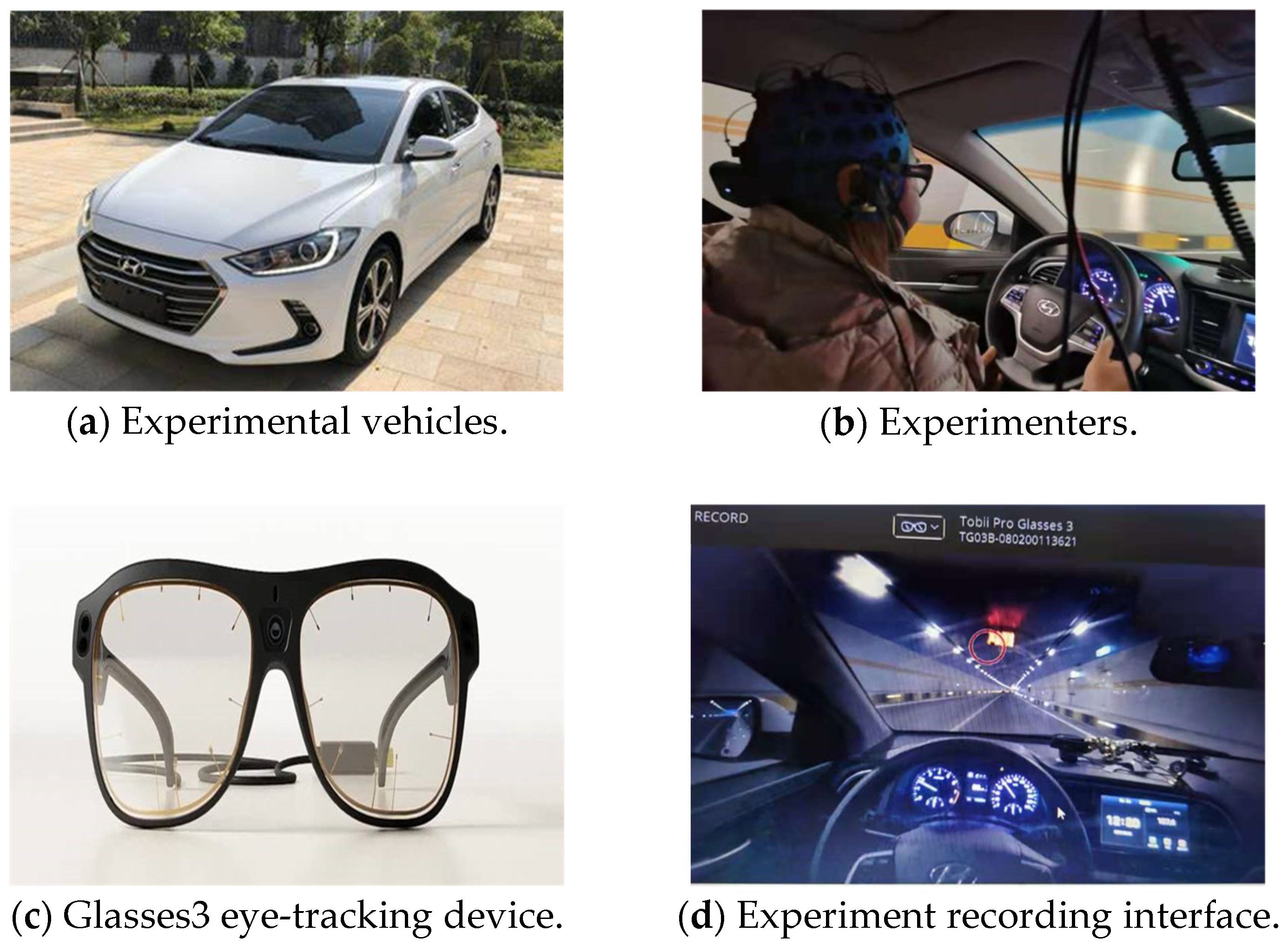
Participants: Forty local drivers of varying ages, genders, occupations, and levels of education were selected as subjects for the experiment. Before participating in the experiment, each driver completed a written consent form and a personal information questionnaire, which primarily included: (1) the driver’s age and gender; (2) the driver’s occupation and driving age; (3) the number of traffic accidents; (4) the driver’s visual acuity or corrected visual acuity level; and (5) the driver’s physical and mental health status. The questionnaire revealed that the age distribution of the sample drivers ranged from 20 to 70 years old (mean = 41.50, standard deviation = 15.56), with thirty males and ten females, and only one male experimenter had more than five traffic accidents. All drivers had more than three years of experience, with ten driving between four and six years and four driving for more than fifteen years. More than half of the test subjects reported that they regularly drove on the highway and were in excellent physical and mental condition during the experiment. The vehicle, acquisition, recording, and output comprise the experimental model’s four components. The practical driving vehicle was an automatic Hyundai Pilot. There were two components to the collection equipment: onboard driving equipment and driver physiological data collection equipment. The vehicle driving equipment consisted of a vehicle self-diagnosis system (OBD), which recorded the driving status and speed of the vehicle, and an illuminance meter, which collected the tunnel data. The driver’s physiological information collection device collected information using the Glasses3 version of a wearable eye-tracking device, which can capture the driver’s visual environment, eye state, and pupil changes and realize the eye dynamic collection function. The recording device consisted of front and rear cameras installed on the interior windshield of the vehicle to capture and record the driving status of the driver. The output device was the ErgoLAB multi-channel data synchronization recording module, which exported synchronous vehicle data, driving behavior, eye movement, physiological, and EEG data. The experimental vehicles, personnel, and instruments are depicted in Figure 2.

2.2. Experimental Procedure

The experimental process began at the Zhangjiakou Chicheng South Toll Station and concluded at the Prince City Toll Station. The line’s total length is 40 km. Round-trip experiments were scheduled at various times throughout the day.
The experiment included a phase of preparation and a phase of formal experimentation. During the preparation phase, we informed the drivers of the requirements and precautions for the investigation while they filled out the questionnaire. Then, we inquired if the driver was experiencing any discomfort or other problems. We then had the test driver wear the equipment and verify that it was properly attached. After properly securing the equipment, the eye-tracking device was calibrated, and the data acquisition system was tested. In preparation for the formal experiment, the staff made a start gesture in front of the camera mirror. Beginning the formal investigation, each device was required to collect the vehicle, tunnel, and driver data simultaneously. To complete the experiment, the driver operated the vehicle according to his or her routine; the staff recorded the conditions using the computerized real-time monitoring equipment. After one test driver completed the experiment and the associated data were saved, the next test driver was prepared to conduct the experiment and complete the formal portion.
Experimental precautions: (1) The subjects were informed in advance of the practical route to exclude outside interference and minimize the physiological and psychological impact of external factors to ensure the data’s accuracy; (2) the driver had to abide by traffic regulations and lane changes, phone use, and other behaviors were prohibited; (3) other personnel in the vehicle had to maintain silence during the experiment.

3. Speed Prediction Modeling and Analysis

3.1. Selection of Data Indicators

In the natural vehicle driving experiment, data regarding the tunnel environment, vehicle braking, and driver physiology were collected. The data collected on the tunnel environment included illumination, the longitudinal road slope, the road friction factor, and the curve radius. Simultaneously, the experiment gathered information regarding vehicle braking, including vehicle speed, steering wheel rotation angle, and braking. The driver’s physiological information included the size and position of their pupils. This study modeled the tunnel exit speed prediction based on the tunnel environment and driver characteristics. The data on vehicle braking and driver physiological information were then analyzed using Pearson’s correlations. A 95% confidence interval indicates a significant negative correlation between the vehicle speed and the illumination index (r = −0.30, Sig. = 0.00). A negative correlation between the vehicle speed and the mean pupil diameter index (r = 0.99, Sig. = 0.00) was statistically significant. Consequently, the tunnel illumination and the driver’s pupil size were selected as model parameters to predict the vehicle speed.

3.1.1. Speed Distribution

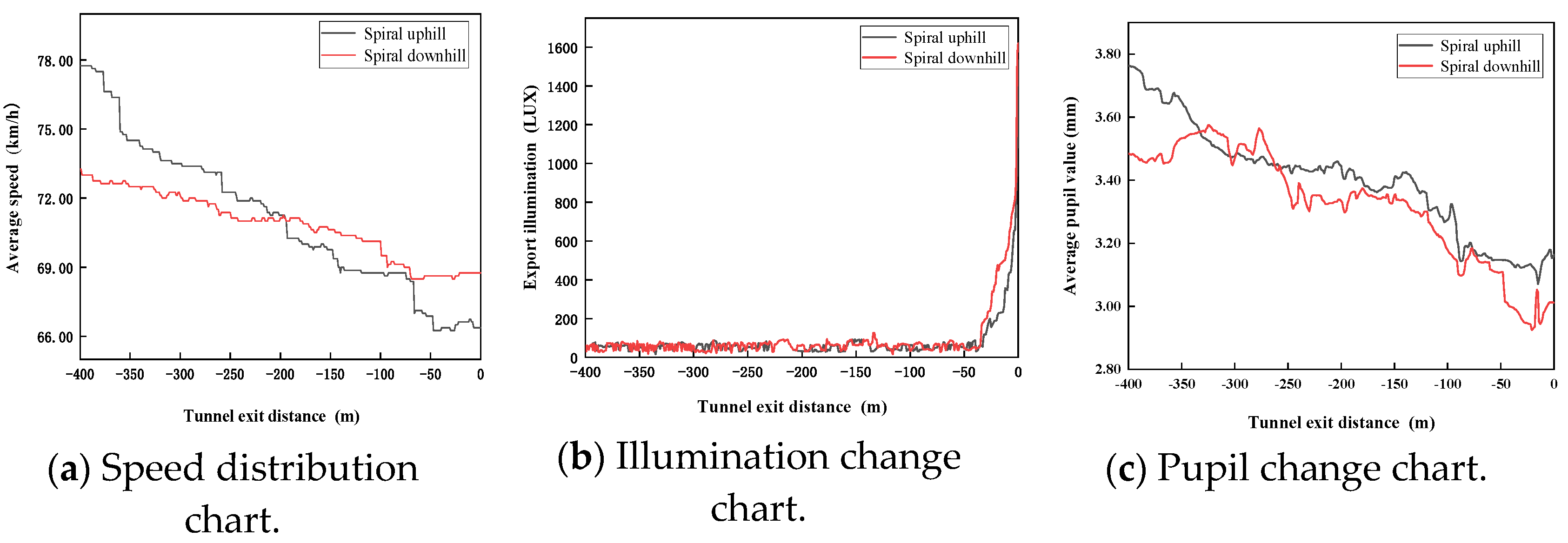
Figure 3a depicts the speed distribution of the tunnel exit phase, where 0 m represents the tunnel exit, the negative sign represents the distance from the tunnel exit, and −400 m to 0 m represents the exit section. The overall speed distribution can be observed. When exiting the tunnel, regardless of whether the driver was on the uphill spiral or the downhill spiral section, the speed decreased. In the spiral ascent phase, the average speed was 71.19 km/h, with a standard deviation of 3.25 km/h, a minimum value of 66.25 km/h, and a maximum value of 77.75 km/h. The average speed during the spiral descent phase was 70.85 km/h, with a standard deviation of 1.42, a minimum of 68.50 km/h, and a maximum of 73.25 km/h. Much more significant was the decrease in the uphill spiral speed compared to the decrease in the downhill spiral speed. In the −400 m to −200 m section of the tunnel exit, the uphill spiral speed was greater than the downhill spiral speed. However, the uphill spiral speed was slower than the downhill spiral speed from −200 m to 0 m at the exit of the tunnel. At −200 m, the uphill and downhill spiral speeds were nearly identical; at −65 m, the uphill spiral speed varied significantly, whereas the downhill spiral speed varied minimally. The difference between the uphill spiral velocity and the downhill spiral velocity was statistically significant (t = 3.68; Sig. = 0.00). When driving out of the tunnel on the downhill spiral, the drivers’ movements were relatively steady. Consequently, the running speed can be utilized as one of the indicators to respond to a shift in the driver’s behavior.

3.1.2. Illumination Change

Figure 3b depicts the change in illumination at the tunnel’s exit. Regardless of whether the tunnel’s spiral was ascending or descending, the overall evolution of illumination reveals a sharp increase in it during the tunnel’s exit phase. The average illuminance during the upward spiral phase was 79 Lux, with a standard deviation of 119, a minimum value of 16 Lux, and a maximum value of 1531 Lux. The average illuminance during the downward spiral phase was 97 Lux, with a standard deviation of 163, a minimum value of 17 Lux, and a maximum value of 1621 Lux. From −400 to −50 m, the illuminance was as low as a few tens of lux. At the tunnel’s exit, the illuminance between −25 m and 0 m reached as high as 1700 Lux, with a significant change at −25 m. The uphill spiral illuminance was significantly more effective than the downhill spiral illuminance, with a significant difference between the two (t = −5.96, Sig. = 0.00). When the drivers exited the tunnel on the uphill spiral, the illumination of the exit section was intense, and the drivers’ visual task was difficult. Therefore, the tunnel exit lighting environment was a crucial indicator of the psychological and behavioral changes among drivers.

3.1.3. Driver Pupil Changes

Figure 3 depicts the pupil diameter analysis of the drivers during the tunnel exit phase (c). As the distance between the vehicle and the entrance of the cave decreased, the uphill and downhill spiral pupil values exhibited a significant decreasing trend. Throughout the uphill spiral phase, the mean pupil size was 3.40 mm, with a standard deviation of 0.18 mm, a minimum of 3.10 mm, and a maximum of 3.80 mm. During the downhill spiral phase, the mean pupil size was 3.33 mm, with a standard deviation of 0.18 mm, a minimum of 2.93 mm, and a maximum of 3.57 mm. There was a significant positive correlation between the mean pupil value of the downhill spiral (r = 0.89, Sig. = 0.00) and the mean pupil value of the downhill spiral (within the 95% confidence interval). During the exit phase of the tunnel, the drivers’ pupils gradually contracted, and the drivers’ mental load and visual task increased [18]. Consequently, the driver pupil value variation was an excellent quantitative indicator of the drivers’ visual adaptation and load level in the spiral tunnel.

3.2. Speed Prediction Model

The speed model is based on the idea that artificial neural networks with feedback memory are capable of self-learning. The illumination and the drivers’ pupils were selected as the tunnel environment and psychological load indicators for constructing a time-series speed prediction model for the exit phase of a spiral tunnel. In order to study driving safety in a long spiral tunnel, it was essential to investigate the significant effects of the tunnel environment changes and the drivers’ psychological load changes.

3.2.1. NARX Model

A nonlinear autoregressive dynamic neural network is NARX. A typical NARX neural network consists of an input layer, a hidden layer, an output layer, and delays at the input and output layers. Figure 4 depicts the basic structure of a NARX neural network.

3.2.2. Model Process and Results

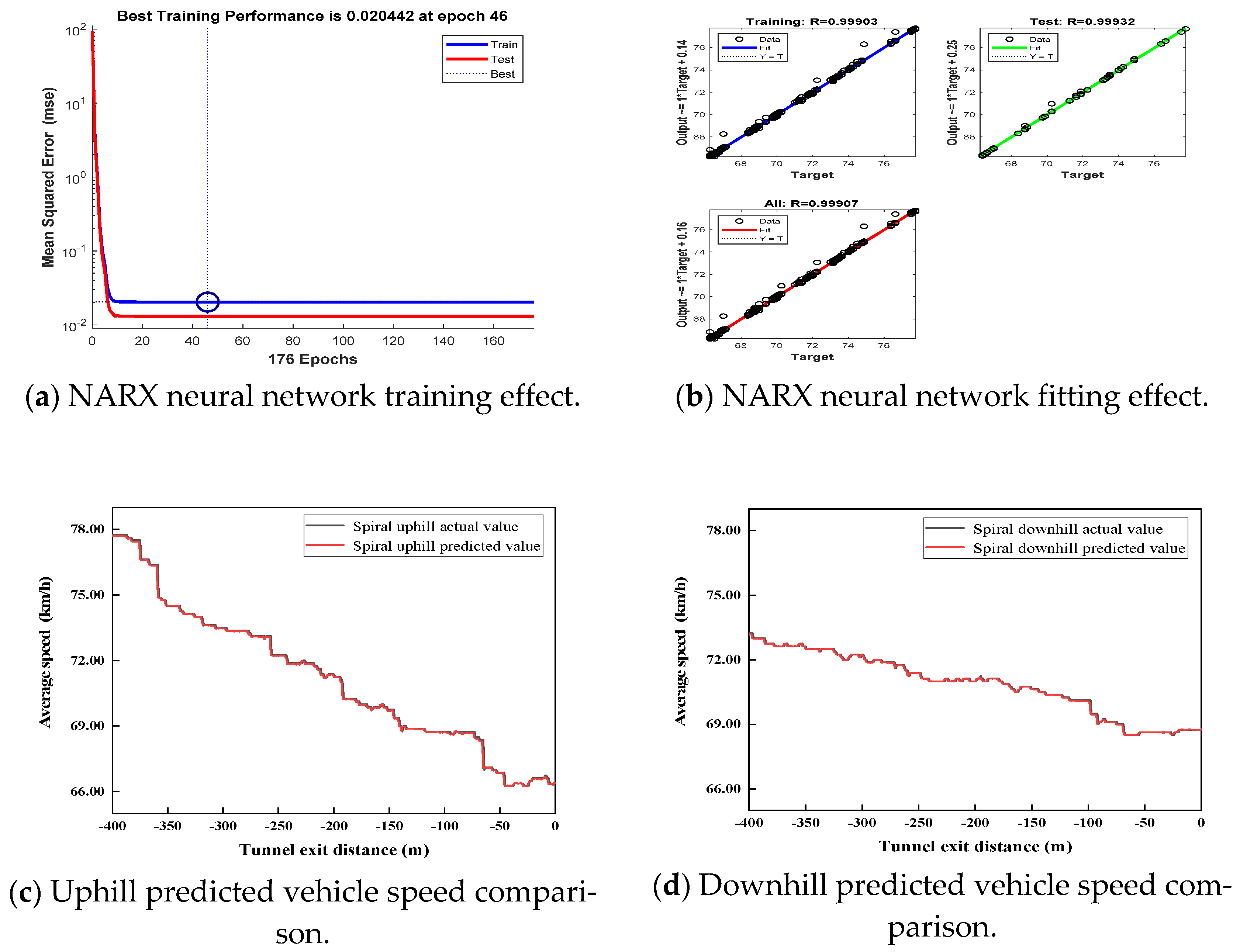
The authors of this paper constructed a time-series NARX neural network model in Matlab using 70% of all the data as training data, 15% as validation data, and 15% as test data. The number of hidden layer neurons and the input and output delays of the network have a substantial effect on the network’s training effect and final prediction performance. After multiple tests, the default value for the number of neurons in the hidden layer was ten. The ratio of the input-to-output delay was 1:2 by default. The weights were updated utilizing the gradient descent method. Figure 5 depicts the impact of the NARX neural network training on the drivers’ performance in the exit segment of an uphill spiral tunnel. As shown in the graph, the validation set error of the NARX neural network increased after 46 training sessions. This indicates the completion of the training. The error of the entire data set was 0.020442, the goodness of fit for all data was 0.999, and the correlation coefficients between the input and error fell within the confidence interval. Therefore, the NARX neural network model accurately predicted the speed of vehicles driven by humans through the exit segment of the uphill spiral tunnel. Similarly, the NARX neural network was used to predict the spiral tunnel’s exit section.
Figure 5 compares the predicted speed of the uphill and downhill spiral slopes of the tunnel exit segment to the actual speed of the vehicle. In the 95% confidence interval, there was a significant positive correlation between the predicted average rate of the uphill spiral and the predicted average speed of the downhill spiral (r = 0.96, Sig. = 0.00). The overall trends of the predicted and actual rates were identical. The predicted average speed on the uphill spiral was 71.16 km/h, with a standard deviation of 3.23, and minimum and maximum values of 66.24 km/h and 77.74 km/h, respectively. The predicted average speed on the downhill spiral was 70.85 km/h, with a standard deviation of 1.41, and minimum and maximum values of 68.50 km/h and 73.21 km/h, respectively.

4. Traffic Safety Risk Evaluation

4.1. Driving Sight Distance Calculation

According to the literature [19], forward-looking time is the amount of time a driver spends visually concentrating on the road ahead and following the expected driving trajectory while maneuvering a vehicle. This metric demonstrates that maintaining the correct running sight distance during the exit phase of a tunnel reduces driving risk and improves driver comfort as the running sight distance changes states more smoothly. Equation (1) demonstrates how to calculate the apparent running distance. The experiment determined that the drivers’ average reaction time during the long tunnel exit phase was approximately 1 s. The formula for calculating the tunnel exit phase look-ahead time is L = V i / 1.3 , where V i represents the predicted driver’s continuous speed change, t represents the driver’s reaction time, the road friction factor f takes the value of 0.65, and the road slope g takes the value of 0.019. A certain critical safety distance l i = 5 m must be considered when braking the vehicle to ensure driving safety. The principle of least-squares enables the fitting of the observed data and the evaluation of the suitability of the selected indicators through curve fitting. Equation (2) is a polynomial coefficient equation y 1 for calculating the driver’s operating sight distance in the tunnel exit phase.
l s = L V i t 3.6 V i 2 254 ( f + g ) l 1
y 1 = 1.477 e 10 x 4 + 1.017 e 7 x 3 + 2.265 x 2 + 0.001 x + 3.152
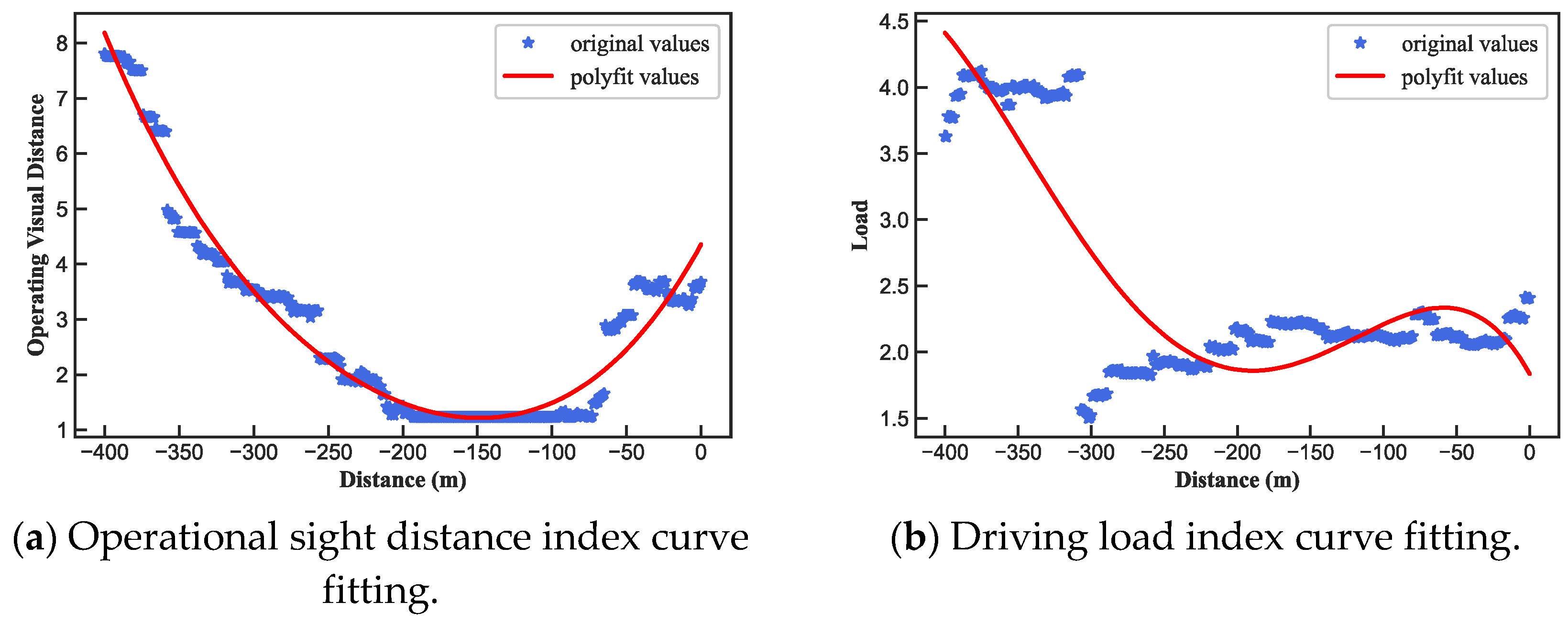
According to the results, the correlation coefficient of the running sight distance curve is R 2 = 0.98, which is the optimal value. As depicted in Figure 6, the tunnel exit operating sight distance demonstrates a decreasing and then increasing trend. From −400 m to −200 m from the tunnel’s exit, the sight distance decreased continuously. The running sight distance was consistent between −200 and −70 m. The operating sight distance increased from −50 m to 0 m.

4.2. Driving Load

According to the literature [20,21], the driving load of a driver is dependent on a number of variables. The greater the load value of driving is, the more anxious the driver becomes and the more unpleasant the driving becomes. The ambitious experiment’s vehicle braking information data analysis reveals a significant negative correlation between the car speed and the steering wheel rotation angle (r = −0.36, Sig. = 0.00). Vehicle speed can best characterize the vehicle’s motion state, so the predicted vehicle speed and the actual steering wheel angle were chosen as the model’s characterization variables. The driving-load variable serves as the dependent variable in the regression model. The regression coefficient of the model was [−0.090, −0.053], and the intercept of the equation was −2.474. The established regression equation is Equation (3). This model demonstrates that the correlation coefficient between the predicted vehicle speed and the actual steering wheel angle on the driving load index was equal to 0.92. Similarly, the principle of least-squares was used to fit the data. Equation (4) is the polynomial coefficient equation for the tunnel exit phase driver load.
y 2 = 0.090 x 1 0.053 x 2 2.474
y 2 = 1.000 e 9 x 4 9.252 e 7 x 3 + 0.0002 x + 1.832
The correlation coefficient for fitting a curve was R 2 = 0.73, which meets the driving load index fitting specifications. As illustrated in Figure 6, the driving load value of the tunnel exit in the −400 m to −300 m segment fluctuated significantly, whereas the driving load value of the tunnel exit in the −300 m to −50 m segment tended to be smooth. As the tunnel exit is approached, the driving load value gradually increased, indicating that the driving load by vehicle braking and the magnitude of the tunnel exit environment changes impact the tunnel exit section.

4.3. Follow Time Distance

As a measure of a driver’s psychological state while driving, the driving load is subjective. Consequently, it does not accurately depict the driver’s driving process in a specific tunnel environment. To objectively evaluate the driver’s state of driving in the tunnel exit section, the predicted speed V i was assumed to be the actual speed in the study. Under the assumption of different control groups, Equation (5) can compute the following time distance D between the rear and front cars.
T H W = D V i
In accordance with the available literature [22], the front vehicle distances D were set to 10, 17.5, and 25 m in order to obtain driver braking data for the tunnel exit section. Figure 7 depicts the variation in the following distance time based on the following distance setting. The subsequent time distance increased gradually as the subsequent distance increased. The length at the tunnel’s exit was negatively proportional to the subsequent time distance. The following distance was shorter the closer the driver was to the entrance. At the vehicle distance of D = 10 m, the mean value of T H W 1 was 0.51 s, the standard deviation was 0.23 s, the minimum value was 0.46 s, and the maximum value was 0.54 s. At the vehicle distance of D = 17.5 m, the mean value of T H W 2 was 0.89 s, the standard deviation was 0.40 s, the minimum value was 0.81 s, and the maximum value was 0.95 s. At the vehicle distance of D = 25 m, the mean value of T H W 3 was 1.27 s, the standard deviation was 0.06 s, the minimum value was 1.16 s, and the maximum value was 1.36 s. Based on the preceding findings, we can conclude that the vehicles maintained a greater distance between them when the following time distance was greater. Thus, the driver will have a greater psychological margin, which will promote the safe operation of the vehicle in tunnel exit traffic.

4.4. K-Means-Based Clustering Analysis of Driving Behavior

4.4.1. Clustering Analysis of Driving Behavior

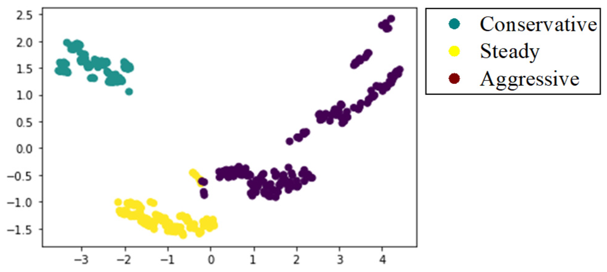
During the exit phase of a tunnel, driver behavior changes varied significantly. Consequently, the K-means cluster analysis algorithm categorizes the classes and evaluates the driving behavior based on various dimensions. As model parameters, the driving running sight distance, the driving load, and the following time distance were chosen to evaluate the road environment and conditions during the tunnel exit phase. This study utilized the K-means algorithm to categorize the driving behavior of drivers in the −400 m to 0 m segment of the tunnel exit into three distinct categories: conservative, smooth, and aggressive. Figure 8 depicts the clustering outcomes. The clustering result is K = 3, and the clustering performance evaluation index profile coefficient is 0.594. This suggests that the clustering performance was satisfactory. In addition, 35% of the samples were conservative, and the behavioral tendencies of the drivers were dynamic. The smooth category comprised 45% of the total sample, and the drivers’ behavioral preferences were average. Finally, 20% of the results were in the aggressive category, and the drivers’ behavioral tendencies were weak.

4.4.2. Driving Behavior Expectations

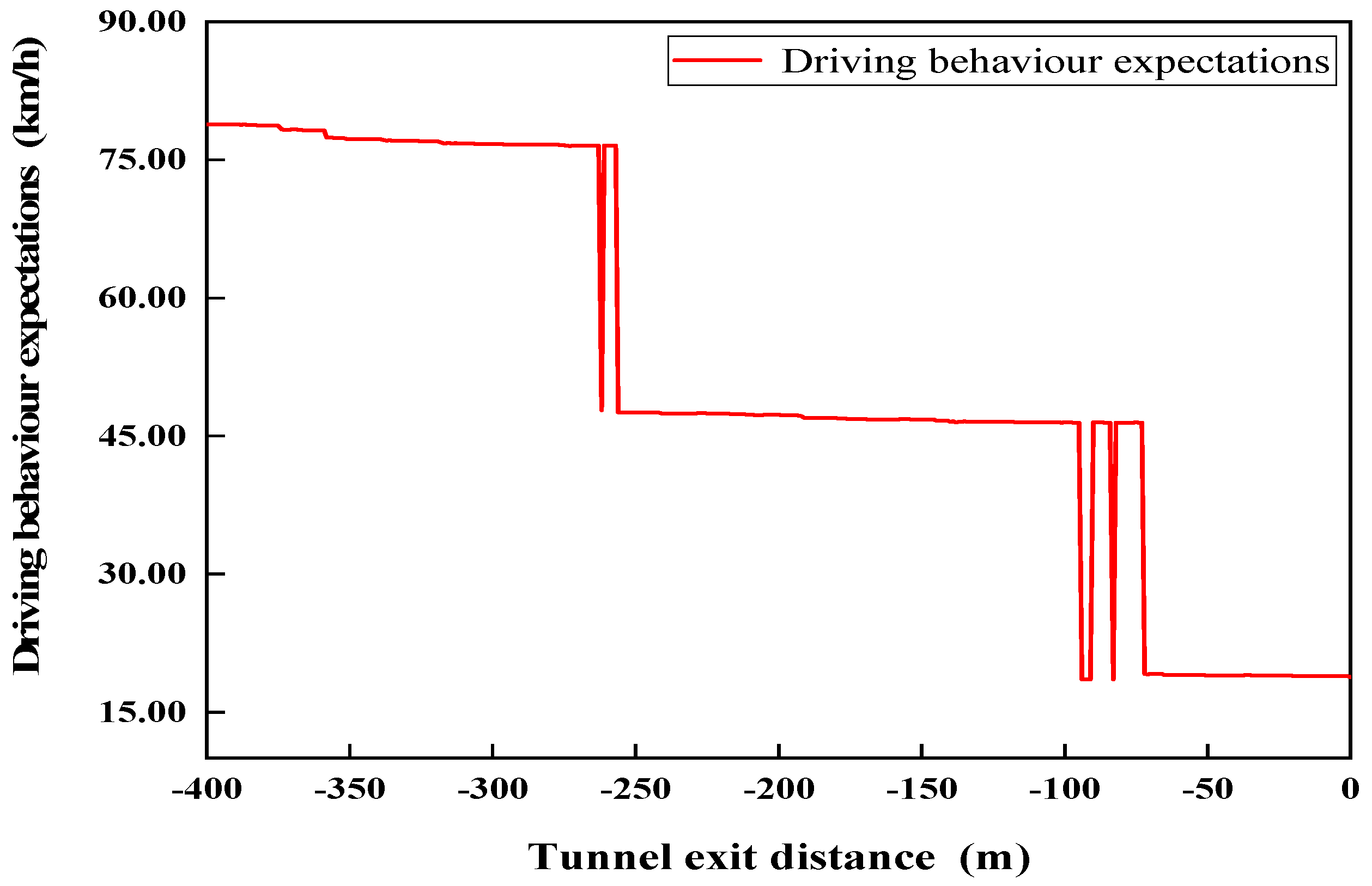
According to the literature [16,17], the subjective evaluation of the driver’s driving behavior during the exit phase of the tunnel can be quantified. Weights were assigned to the types of driving behavior identified by the cluster analysis. This paper denotes the driver behavior factor K as 0.8 for the conservative type, 0.5 for the smooth type, and 0.2 for the aggressive type. The greater the value of K, the more stable the driver’s state of driving is in the tunnel section. Based on the psychological load, safety, and other considerations, the driving behavior expectation L can reflect the driver’s maximum regular speed. Using v 0 (the model-predicted rate) and v * (the experimental tunnel section speed limit of 80 km/h), we can calculate the expected driving behavior for the tunnel exit phase using Equation (6).
L x = K × 50 ( 1 + V 0 V * )
The tunnel exit phase driving behavior expectation shows a downward gradient trend, as shown in Figure 9. At −400 m to −250 m, the driving expectation value decreased from 78.87 km/h to 47.57 km/h. At −265 m to −250 m, the driving expectation value fluctuated from 47.57 to 76.55 km/h. Between −250 m and −100 m, the driving expectation value remained at 46.97 km/h. The driving expectation fluctuated from 18.58 to 46.47 km/h from −100 m to −75 m. At −75 m to the exit, the driving expectation of 18.98 km/h remained stable. This shows a significant change in the driving behavior expectations considering the driver behavior factor.

4.5. Tunnel Exit Phase Predicted Speed Analysis

Critical Safety Distance Based on the Predicted Speed of the Exit Phase
Based on the literature [23] and combined with Equation (7) for the tunnel driving environment, the critical safe speed value of V 0 = 100.2157 km/h was obtained for the exit section of the tunnel. The exit phase predicted speed clustering analysis yielded three clustering center speed distributions at 80 km/h, 73 km/h, and 68 km/h, and all were lower than the critical safe speed.
V 0 = 127 f [ 1 1.2 t 3.6 + ( 1 1.2 t 3.6 ) 10 127 f ]
According to Equations (8) and (9), we can obtain the critical safety distance S 0 and critical warning safety distance S 1 for the exit section of the tunnel.
S 0 = 1 36 ( t 2 + t 3 2 ) V 0 + V 0 2 25.92 f G + d 0
S 1 = V 0 t + 1 3.6 ( t 2 + t 3 2 ) V 0 + V 0 2 25.92 f G + d 0
The interpretation of the parameters in the formula is shown below: V 0 critical safety speed for the exit section of the tunnel; f road friction coefficient 0.65; t driver reaction time of 1 s; t 2 braking delay time 0 s; t 3 time taken to increase the deceleration from 0 to the maximum deceleration of 0.2 s; G gravitational acceleration of 9.8 m/s2; d 0 he minimum safety distance that should be maintained with the obstacle vehicle after the main vehicle has stopped is 0.1 m.
For the exit section of the tunnel, the critical safety speed and the safety distance of the rate at the center point of the K-means clustering were calculated, respectively. Both the acute and warning safety distances decreased as the vehicle’s speed decreased. Table 1 displays the safe passing distance reference for the tunnel exit section.

4.6. Tunnel Exit Phase Speed Control Measures

The driving behavior expectation distance, critical safety distance, and warning safety distance were selected as the input layer variables. This study used the predicted operating speed as the simulation label for a BP neural network and the variable speed limit as the output [24]. This allows for reasonable speed control during the tunnel’s exit phase. To ensure the continuity of the vehicle’s running speed on the tunnel exit section, the tunnel exit segment was divided into various speed limit intervals. The running speed difference between the tunnel sections was reduced to have a restraining effect on small car drivers, forcing them to slow down in advance of the tunnel exit section.
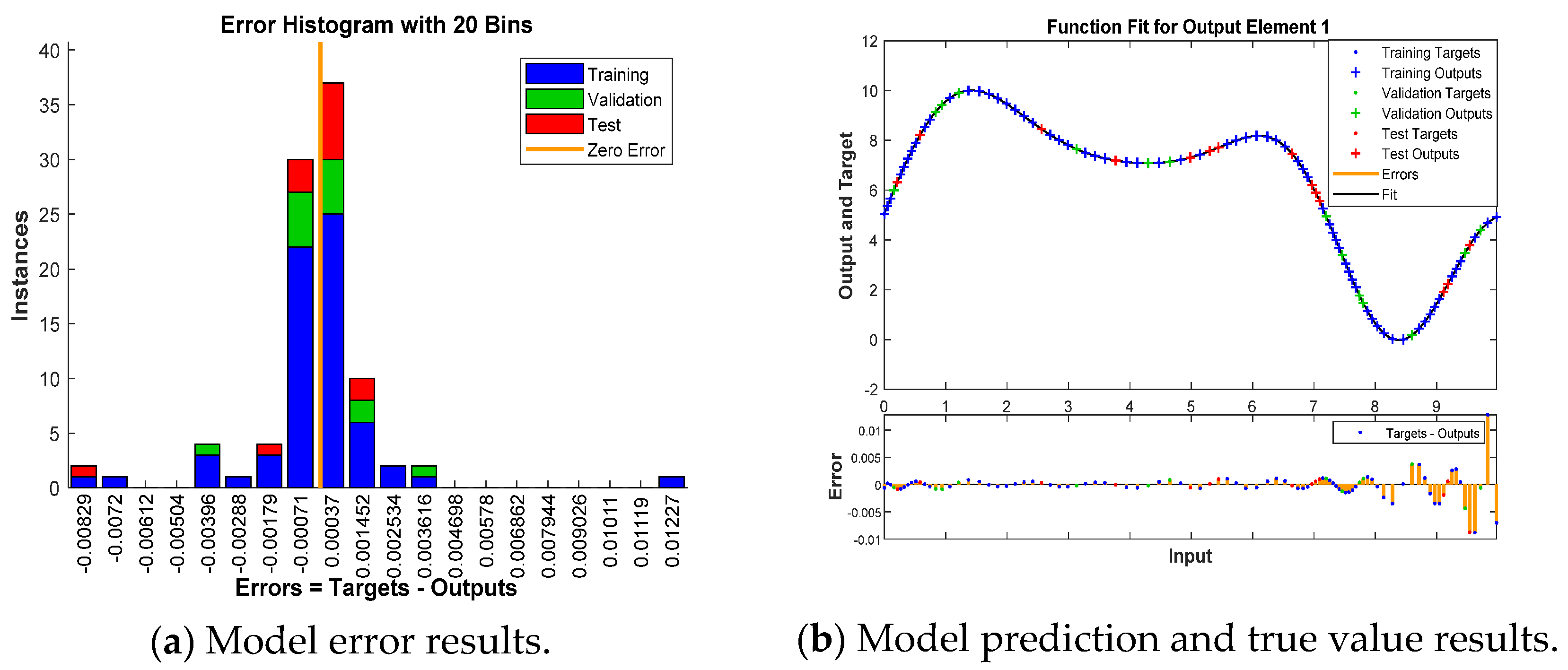
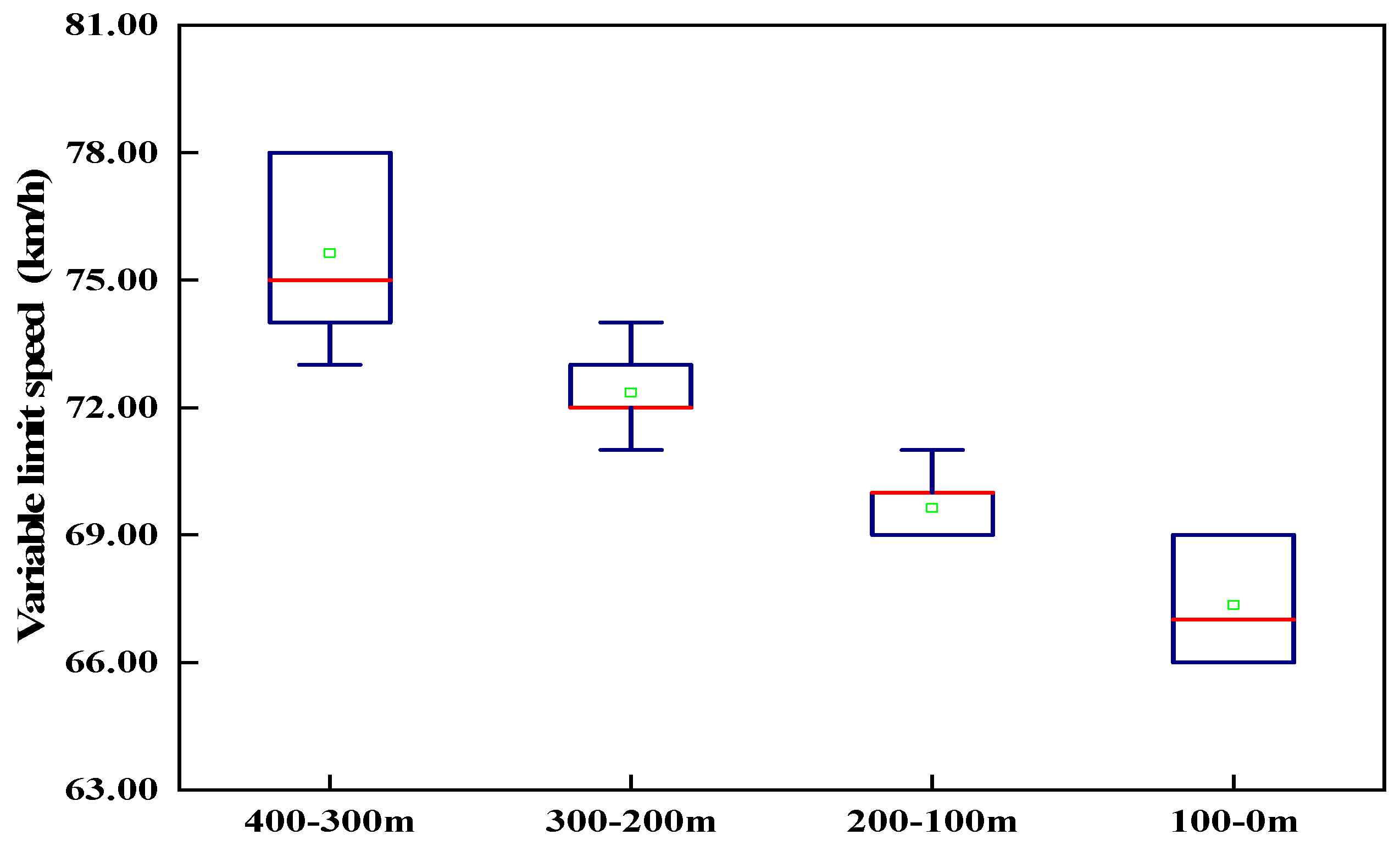
Figure 10a demonstrates that after training the BP neural network, the error of the entire data set was 0.0067315, and the goodness-of-fit for all data was 0.999. Figure 10b illustrates the overall model outcomes. The input and error correlation coefficients fell within the confidence interval. Consequently, the BP neural network model was used to accurately predict the variable speed limit for drivers in the tunnel exit section. Figure 11 depicts the outcomes of the variable speed limit at various intervals during the tunnel’s exit phase. Derived in the distance from the tunnel exit section from −400 m to −300 m, the drivers’ speed control was set to 75 km/h. In the distance between −300 m and −200 m from the tunnel exit, the drivers maintained a speed of 72 km/h. From −200 m to −100 m from the tunnel exit, the drivers’ driving speed control was 70 km/h. At a distance of −100 m from the tunnel exit, the drivers maintained a speed of 67 km/h. From −400 m to 0 m, the entire interval speed average was 71 km/h, and the variable speed limit was lower than the 80 km/h Jinjiazhuang spiral tunnel speed limit. The use of variable speed limits allowed the drivers to maintain a smooth level of comfort during the exit phase of the tunnel and reduced the risk of traffic accidents in the tunnel’s exit section by limiting the speed during the exit phase.

5. Conclusions

The authors of this paper investigated the speed prediction model in the exit phase of the tunnel, selected the Jinjiazhuang spiral tunnel for a natural vehicle experiment, explored the change law of driving behavior in the exit phase of the helical tunnel, established a NARX speed prediction model based on driver characteristics at the exit phase of the spiral tunnel, and performed cluster analysis on driving behavior. The authors also investigated the changes in driver speed and the laws of driving behavior in the tunnel’s exit phase. This study provides research to ensure traffic safety in tunnels’ exit phases.
The following is a summary of the conclusions reached in this study:
(1)
The driver is influenced by the exit environment. Under extreme concentration, the driving load fluctuates noticeably. According to an analysis of the tunnel exit section’s driver characteristics and environmental features, the vehicle’s speed decreased continuously during both the uphill and downhill spiral phases in the tunnel exit section. Due to the effect of road alignment, the uphill spiral speed decreased more gradually than the downhill spiral speed. As the illumination of the tunnel’s exit section fluctuated drastically, causing the drivers’ pupils to contract rapidly, the drivers’ field of vision constantly decreased. The drivers slowed down during vehicle braking, and load fluctuations caused changes in the environment. The substantial influence of ecological illumination on the drivers during the tunnel exit phase has a negative effect on traffic safety [25].
(2)
During the tunnel’s exit phase, the drivers’ driving behavior and driving expectations changed significantly. During the tunnel exit phase, the reduced visual range and fluctuating driving load significantly altered the drivers’ behavior. The closer a driver was to the exit, the more aggressive their driving behavior became. Taking into account behavioral factors in driving expectations revealed a downward trend in driving expectations. 75 m before tunnel exit, the expected speed was as low as 18.98 km/h. This demonstrates that effective control of the drivers’ speed during the tunnel’s exit phase had a significant impact on traffic safety during the tunnel’s exit phase.
(3)
Setting dynamic safety and comfort speeds to keep drivers comfortable during the tunnel exit phase can effectively reduce tunnel exit traffic risk. Taking into account significant differences in the environmental impact and substantial changes in driver characteristics during the tunnel exit phase, setting variable speed limits within the safe driving speed tolerance range and decreasing speed dispersion is advantageous to the safe operation of tunnel exit phase traffic.
In conclusion, the unique small radius and continuous longitudinal slope of the particular road alignment of the long spiral tunnel pose certain safety risks for vehicle braking and driver behavior. By controlling the speed of the tunnel’s exit phase in a reasonable manner, traffic safety risks associated with drivers’ increased unconscious acceleration and deceleration due to environmental changes can be reduced. Setting variable speed limit control measures to minimize the psychological load of drivers closer to the exit distance can protect driver safety during the tunnel exit phase.

6. Discussions and Perspectives

Despite the fact that this paper presents an analysis of the behavioral changes of drivers during the exit phase of a spiral tunnel based on natural vehicle experimental data and proposes a reference value for the tunnel exit section speed, there are issues with the limited sample interval data, the relatively low traffic flow, and insufficient control of the variables. In a subsequent study, therefore, we will combine the simulation experiment method with the tunnel data collection to further investigate the spiral tunnel driver driving risk.
With the rapid development of data mining techniques, such as driver physiological data and vehicle handling behavior, the technical means to evaluate and predict human factors in the “human–machine–environment” system in real time are becoming more sophisticated. Under the guiding principles of “people-oriented”, dynamic monitoring, control, and intervention of drivers’ human risk levels (including physiological and psychological states and driving-behavioral risk states), real-time dynamic variable speed limits can effectively reduce traffic accidents and enhance road safety levels. Assessing and predicting the risk state of drivers in real time can aid in the design and development of intelligent driving assistance systems.

Author Contributions

Formal analysis, S.Z.; investigation, X.W.; writing—original draft, X.X.; writing—review & editing, X.X. and C.S.; supervision, X.K. All authors have read and agreed to the published version of the manuscript.

Funding

This research was funded by the Foundation of State Key Laboratory of Mechanical Behavior and System Safety of Traffic Engineering Structures (No. ZZ2020-03), Hebei Natural Science Foundation (No. E2019210305), Foundation of S&T Program of Hebei (No. 20557673D), and 2022 Hebei Province, the Introduction of Foreign Intellectual Projects.

Institutional Review Board Statement

Not applicable.

Informed Consent Statement

Informed consent was obtained from all subjects involved in the study.

Data Availability Statement

Data are not publicly available, though the data may be made available on request from the corresponding author.

Conflicts of Interest

The authors declare no conflict of interest.

References

  1. Aarts, L.; Schagen, I.V. Driving speed and the risk of road crashes: A review. Accid. Anal. Prev. 2006, 38, 215–224. [Google Scholar] [CrossRef]
  2. Avijit, M.; Tyagi, A. Speed prediction models for car and sports utility vehicle at locations along four-lane median divided horizontal curves. J. Mod. Transp. 2018, 26, 278–284. [Google Scholar] [CrossRef] [Green Version]
  3. Bassani, M.; Catani, L.; Salussolia, A. A Driving Simulation Study to Examine the Impact of Available Sight Distance on Driver Behavior Along Rural Highways. Accid. Anal. Prev. 2019, 131, 200–212. [Google Scholar] [CrossRef] [PubMed]
  4. Cooper, J.M.; Medeirosward, N.; Strayer, D.L. The impact of eye movements and cognitive workload on lateral position variability in driving. Hum. Factors J. Hum. Factors Ergon. Soc. 2013, 55, 1001–1014. [Google Scholar] [CrossRef] [PubMed] [Green Version]
  5. Cai, X.; Lei, C.; Peng, B. Road Traffic Safety Risk Estimation Based in Driving Behavior and Information Entropy. China J. Highw. Transp. 2020, 33, 190–201. [Google Scholar] [CrossRef]
  6. Chen, Z.; Wang, X.; Zhang, X. Modeling of Driver Acceleretion and Deceleration Behavior in Mountain Freeways. China J. Highw. Transp. 2020, 33, 167–175. [Google Scholar] [CrossRef]
  7. Du, Z.; Pan, X.; Yang, Z. Research on Visual Turbulence and Driving Safety of Freeway Tunnel Entrance and Exit. China J. Highw. Transp. 2007, 20, 101–105. [Google Scholar] [CrossRef]
  8. Du, Z.; Pan, X.; Guo, X. Evaluation Index’s Application Studies on Safety at Highway Tunnel’s Entrance and Exit. J. Tongji Univ. Nat. Sci. 2008, 3, 325–329. [Google Scholar]
  9. Figueroa, A.M. Subjective and Objective Risks Consideration in Modeling Highway Safety; Purdue University: West Lafayette, IN, USA, 2005. [Google Scholar]
  10. Guo, K. Car Manoeuvring Dynamics; Jilin Science and Technology Press: Changchun, China, 1991. [Google Scholar]
  11. Guo, Z.; Dai, Y.; Zhou, X. Critical Safety Speed and Its Application Research on Risk Characteristic Section of Expressway Tunnel (Tunnel Group). China J. Highw. Transp. 2010, 23, 116–122. [Google Scholar] [CrossRef]
  12. Guo, Q.; Wang, X.; Chen, Z. Modeling Operation Speed in Mountainous Freeways: A Driving Simulator Study. J. Tongji Univ. Nat. Sci. 2019, 47, 1004–1010. [Google Scholar]
  13. Huang, J.; Ji, Z.; Peng, X. Driving Style Adaptive Lane-changing Trajectory Planning and Control. China J. Highw. Transp. 2019, 32, 226–239+247. [Google Scholar] [CrossRef]
  14. Lamm, R. Possible design procedure to promote design consistency in highway geometric design on two lane rural roads. Transp. Res. Rec. 1998, 1195, 111–122. [Google Scholar] [CrossRef]
  15. Reyes, M.L.; Lee, J.D. Effects of Cognitive Load Presence and Duration on Driver Eye Movements and Event Detection Performance. Transp. Res. Part F: Traffic Psychol. Behav. 2008, 11, 391–402. [Google Scholar] [CrossRef]
  16. Shang, R.; Zhang, S. A Study on Tunnel Traffic Security System of Expressway. Highway 2006, 12, 127–130. [Google Scholar]
  17. Wang, Q. Variable Speed Limit Control for Long Freeway Tunnel Entrances and Exits. Master’s Thesis, Chang’an University, Xi’an, China, 2015. [Google Scholar]
  18. Wang, X.; Chen, Z.; Guo, Q. Transferability Analysis of the Freeway Continuous Speed Model. Accid. Anal. Prev. 2021, 151, 105944. [Google Scholar] [CrossRef] [PubMed]
  19. Xu, J.; Sun, Z.; Long, Y. Study on car following characteristics of minibus across River Bridge Based on natural driving data. China J. Highw. Transp. 2021, 34, 1–13. [Google Scholar] [CrossRef]
  20. Yang, Y. Study on the Minimum Following Distances of Vehicles on Freeway. Master’s Thesis, Chang’an University, Xi’an, China, 2016. [Google Scholar]
  21. Yang, Y.; Chen, Y.; Wu, C. Effect of Highway Directional Signs on Driver Mental Workload and Behavior Using Eye Movement and Brain Wave. Accid. Anal. Prev. 2020, 146, 105705. [Google Scholar] [CrossRef]
  22. Yuan, Q.; Yan, N.; Hao, W. Research on pedestrian risk assessment and early warning algorithm based on psychological safety distance. China J. Highw. Transp. 2021, 34, 1–14. [Google Scholar] [CrossRef]
  23. Zhu, T.; Wu, L.; Hu, Y. Research on Characteristics of Drivers’ Mental Workload in Extra-long Expressway Tunnels Based on the Factor Model. China J. Highw. Transp. 2018, 31, 165–175. [Google Scholar]
  24. Zhao, X.; Ju, Y.; Li, J. Evaluetion of the Effect of PRMs in Extra-long Tunnels Based in Driving Behavior and Visual Characteristics. China J. Highw. Transp. 2020, 33, 29–41. [Google Scholar] [CrossRef]
  25. Zheng, L.; Qiao, X.; Ni, T. Car-following Behavior of Passenger Cars on River Crossing Bridge Based on Naturalistic Driving Data. China J. Highw. Transp. 2021, 34, 240–250. [Google Scholar] [CrossRef]
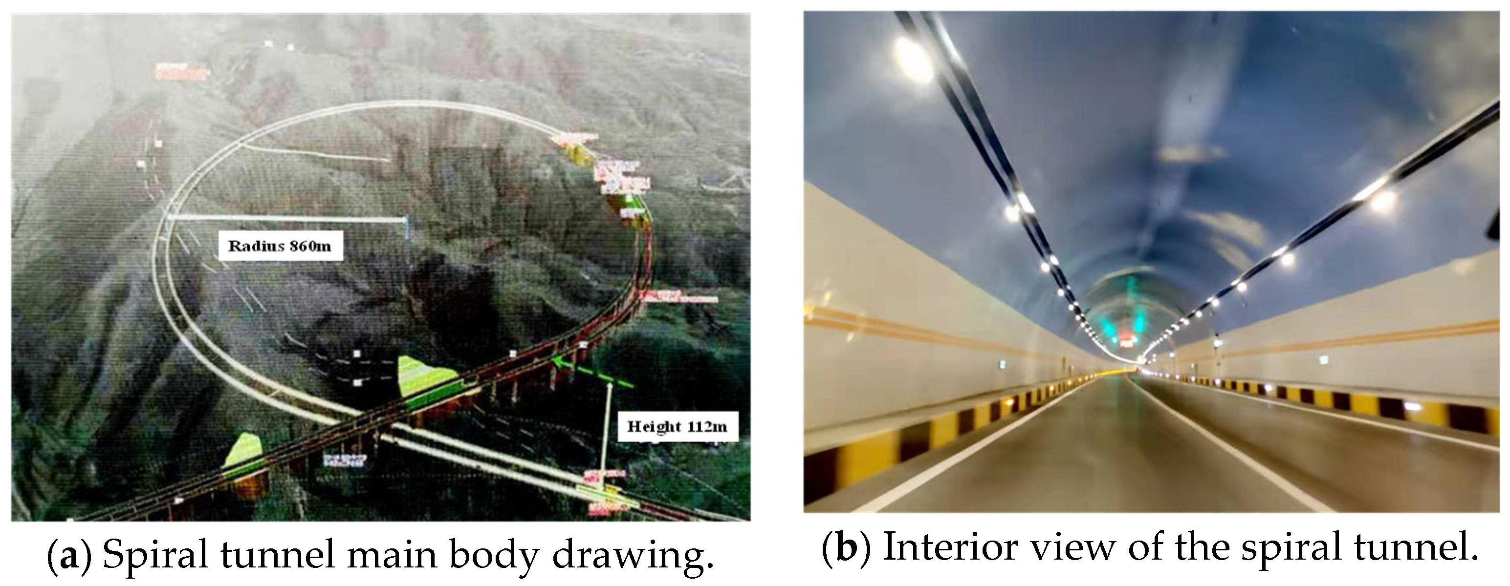
Figure 1. Spiral tunnel diagram.
Sustainability 14 15736 g001
Figure 2. Experimental equipment diagram.
Sustainability 14 15736 g002
Figure 3. Changes in speed and illuminance at the exit phase of the tunnel.
Sustainability 14 15736 g003
Figure 4. The basic structure of a NARX neural network.
Sustainability 14 15736 g004
Figure 5. Tunnel exit prediction speed model result graph.
Sustainability 14 15736 g005
Figure 6. Curve fitting diagram of operation sight distance and driving load index.
Sustainability 14 15736 g006
Figure 7. THW changes under the set pitch of the car.
Sustainability 14 15736 g007
Figure 8. Driving behavior clustering results.
Sustainability 14 15736 g008
Figure 9. Expected changes in driving behavior during the tunnel exit phase.
Sustainability 14 15736 g009
Figure 10. BP neural network model results.
Sustainability 14 15736 g010
Figure 11. Variable speed limit values in different intervals of the tunnel exit phase.
Sustainability 14 15736 g011
Table 1. Safety distances of the tunnel exit phase.
Vehicle Speed (km/h)Critical Safety Distance (m)Early Warning Safety Distance (m)
100.215763.713163.929
8041.086121.086
7334.404107.404
6829.99697.996
Publisher’s Note: MDPI stays neutral with regard to jurisdictional claims in published maps and institutional affiliations.