Article

Energy Demand of the Road Transport Sector of Saudi Arabia—Application of a Causality-Based Machine Learning Model to Ensure Sustainable Environment

1
Department of Civil and Environmental Engineering, College of Engineering, King Faisal University, Al-Ahsa 31982, Saudi Arabia
2
Applied Research Center for Environment & Marine Studies, King Fahd University of Petroleum & Minerals (KFUPM), Dhahran 31260, Saudi Arabia
3
Interdisciplinary Research Center for Renewable Energy and Power Systems, King Fahd University of Petroleum & Minerals, Dhahran 31261, Saudi Arabia
4
Climate Change Response Unit, Wellington City Council, 113 The Terrace, Wellington 6011, New Zealand
5
Department of Civil Engineering, College of Engineering, University of Bahrain, Isa Town P.O. Box 32038, Bahrain
6
Department of Civil and Environmental Engineering, University of Utah, 110 Central Campus Drive, MCE-1435, Salt Lake City, UT 84112, USA
7
Department of Civil and Environmental Engineering, King Fahd University of Petroleum & Minerals (KFUPM), Dhahran 31260, Saudi Arabia
8
Electrical Engineering Department, King Fahd University of Petroleum & Minerals, Dhahran 31261, Saudi Arabia
*
Authors to whom correspondence should be addressed.
Sustainability 2022, 14(23), 16064; https://doi.org/10.3390/su142316064
Submission received: 18 September 2022 / Revised: 28 November 2022 / Accepted: 29 November 2022 / Published: 1 December 2022
(This article belongs to the Special Issue Renewable Energy and Greenhouse Gas Emissions Reduction)

Abstract

:
The road transportation sector in Saudi Arabia has been observing a surging growth of demand trends for the last couple of decades. The main objective of this article is to extract insightful information for the country’s policymakers through a comprehensive investigation of the rising energy trends. In the first phase, it employs econometric analysis to provide the causal relationship between the energy demand of the road transportation sector and different socio-economic elements, including the gross domestic product (GDP), number of registered vehicles, total population, the population in the urban agglomeration, and fuel price. Then, it estimates future energy demand for the sector using two machine-learning models, i.e., artificial neural network (ANN) and support vector regression (SVR). The core features of the future demand model include: (i) removal of the linear trend, (ii) input data projection using a double exponential smoothing technique, and (iii) energy demand prediction using the machine learning models. The findings of the study show that the GDP and urban population have a significant causal relationship with energy demand in the road transportation sector in both the short and long run. The greenhouse gas emissions from the road transportation in Saudi Arabia are directly proportional to energy consumption because the demand is solely met by fossil fuels. Therefore, appropriate policy measures should be taken to reduce energy intensity without compromising the country’s development. In addition, the SVR model outperformed the ANN model in predicting the future energy demand of the sector based on the achieved performance indices. For instance, the correlation coefficients of the SVR and the ANN models were 0.8932 and 0.9925, respectively, for the test datasets. The results show that the SVR is better for predicting energy consumption than the ANN. It is expected that the findings of the study will assist the decision-makers of the country in achieving environmental sustainability goals by initiating appropriate policies.

1. Introduction

The unprecedented increase in global energy demand requires advanced and comprehensive analyses of energy drivers at national, regional, and international levels. The correlation between energy demand and its independent factors can be understood using econometric methods [1,2,3]. The results of causal analysis help understand the most important factor of energy demand and assist in accurately estimating future energy demand. It is essential to estimate future energy demand as it has significant policy implications regarding energy security and future economic growth patterns. Recent developments in computing technology, intelligent forecasting methodologies, and algorithms have paved the way for a major breakthrough in modeling and simulation. Machine learning models regress energy demand using socio-economic, demographic, and climatic variables. Typically, these variables are nonlinear. Therefore, energy modeling became a critical issue for practitioners and scientists to contribute to creating sound plans and policies. One of the crucial steps in energy planning is to assess current energy use and forecast future needs [4,5].
Road transportation is one of the major energy consumption sectors in Saudi Arabia [6]. Since renewable energy resources are not used on a large scale in Saudi Arabia for road transportation, it results in continuous increases in the domestic consumption of petroleum products and the associated increase in greenhouse gas (GHG) emissions. The residents of rich urban areas tend to rely on personal automobiles for most of their travel needs [7]. Saudi Arabia has the highest vehicle ownership in the Middle East [8]. The recent royal decree on allowing women to drive will put 9 million potential new drivers on the road [9]. This increasing number of cars will significantly increase the energy demand in road transportation. Future energy demand can be met by analyzing the factors that have historically influenced energy use and making more accurate predictions based on these factors and historical trends. Econometrics techniques can help to find the key drivers from a set of drivers [10]. However, concerning future demand estimation, the traditional regression method cannot address the nonlinearity of different energy demand components. Previous studies suggested adjusting nonlinearity while dealing with energy consumption [11]. Therefore, it is crucial for the Kingdom to investigate the energy demands of road transportation with cutting-edge methods that will enlighten policymakers and decision-makers.
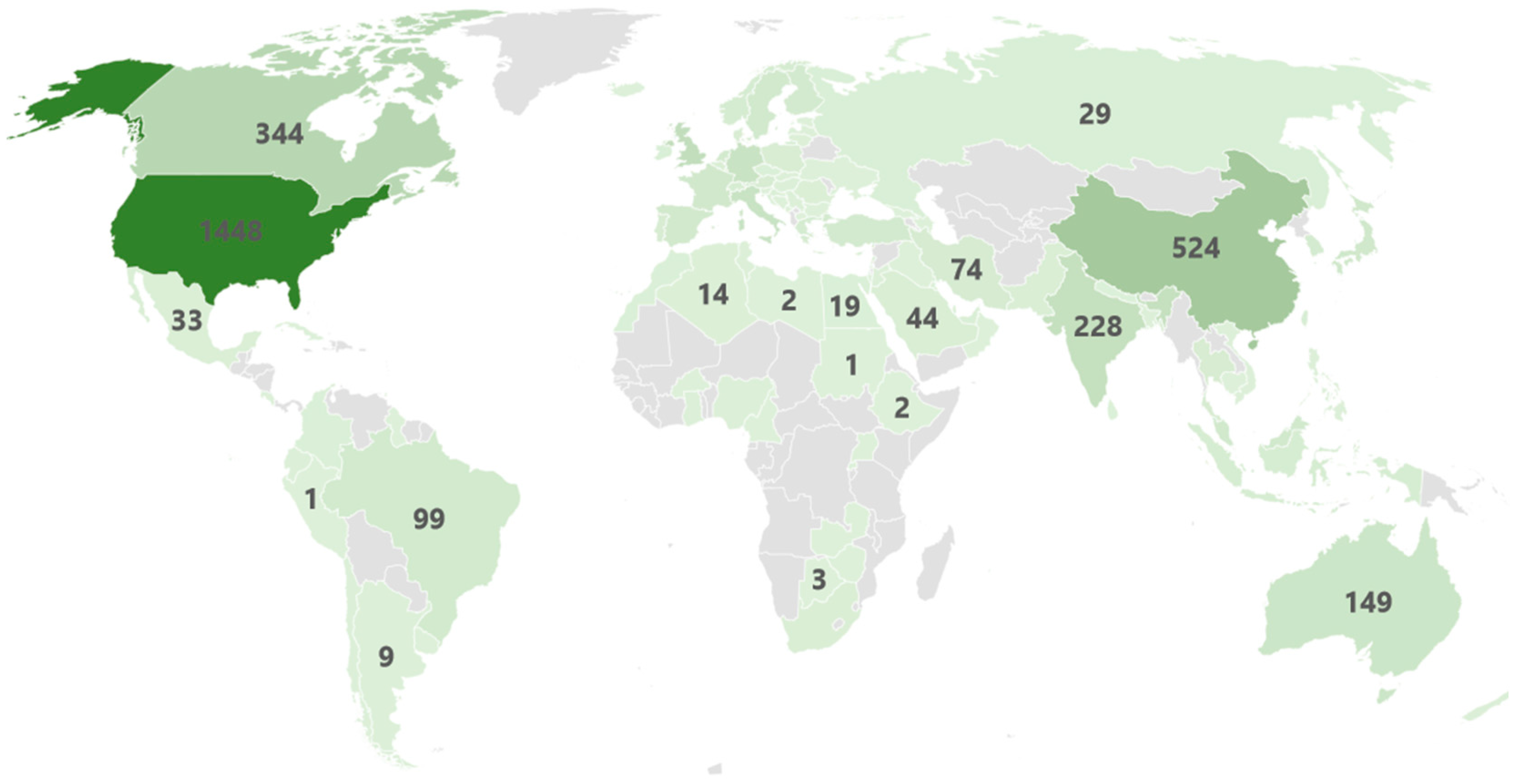
In the relevant literature, the researchers considered different combinations of many variables, which include GDP, gross national product (GNP), population, transport amount (vehicle-kilometer), freight transport amount (ton-kilometer), passenger transport amount (person-kilometer), number of registered vehicles, urbanization rate, and fuel price for developing transport energy models [12,13,14,15,16,17]. Multivariate, cointegration, and regression analysis can explain the influence of different indicators on energy demand. In Ref. [18], a few selected countries investigated the causal interrelationship between energy consumption and GDP. Ozturk and Acaravchi [19] studied the impact of energy use on GDP growth. Canyurt et al. [20] proposed an energy model using a genetic algorithm, selecting GDP, population, and import and export as inputs. Geem [14] proposed a neural network energy model for South Korea. Azadeh et al. [21] reported a fuzzy regression algorithm based Iranian energy model. Denoised electricity demand data allowed An et al. [22] to isolate the seasonal component and use it to train an ANN model. Uzlu et al. [23] used data on Turkey’s GDP, population, imports, and exports to inform a neural network approach to optimizing the country’s energy demand. Deshani et al. [24] took the first difference of the input series. They used a k-means clustering technique to select ANN model inputs for the prediction of the electricity demand. Table A1 in the Appendix A section summarizes various methodologies employed in literature to model energy demand in general and transportation energy demand. Figure 1 presents the article distribution of different countries worldwide based on the results received in Scopus with the keyword-transportation energy demand from the year 2000 to 2022. In contrast, Figure 2 presents the results obtained with the keywords transportation energy demand and greenhouse gas emissions for the same period. It was also evident from the search that the number of publications over the years are growing almost exponentially due to the importance of the topic.
However, according to information presented in Table A1, it was revealed that a significant trend toward applying artificial intelligence (AI) and other regression techniques in energy demand modeling in the transport sector globally. The artificial neural networks approaches are most popular amongst various AI methods. On the other hand, support vector regression, another dominant AI model, has not been explored frequently to model transportation energy demand. However, the SVR requires fewer parameters than other AI models and reaches the global optimum solution at a lower expense. It also does not suffer from the overfitting problem [25]. Due to its benefits, it has been employed in research and industries for decades [26,27,28,29]. This approach was successfully used in a wide range of applications such as building energy consumption [30], energy performance [31], solar radiation [32], and electricity load [33]. Successful application of SVR was also found in transportation engineering and planning; for instance, it was used in intelligent transportation systems [34], retro-reflectivity degradation of traffic signs [35], short-term travel time [36], electric vehicle charging duration time [37], freeway speed [38], and real-time crash risk on urban expressways [39]. In Saudi Arabia’s context, there is a dearth of research on energy demand modeling in the transportation sector of Saudi Arabia that makes use of AI methods. In addition, to the best of the author’s knowledge, the support vector regression is yet unexplored for Saudi Arabia’s transportation energy modeling. Considering the mentioned notes, this article develops a causality-based machine-learning scheme for modeling the energy demand in the transport sector of Saudi Arabia. The significant contributions of the article are as follows:
  • This research employs a vector error correction model (VECM) for causality test analysis to identify a short and long-term relationship between the dependent and explanatory variables;
  • This paper develops an SVR model for forecasting energy consumption in the Kingdom’s road transportation between 2018 and 2030 using a double exponential smoothing method using the projected input dataset.
  • Finally, it compares the results from the SVR model with an ANN model to identify a suitable model for Saudi Arabia’s energy demand in the transportation sector. The ANN model is chosen for comparison purposes due to its popularity in transportation sector energy demand modeling.
The following sections of the article are organized as follows: Section 2 provides a methodology that includes model development data, causality analysis approach, and prediction approach. Section 3 illustrates the results associated with causality analysis and energy demand projection models. Finally, the article is concluded in Section 4 with policy implication-related remarks.

2. Methodology

This section briefly discusses the data used for the development of AI-based energy demand models in the transport sector of Saudi Arabia. In addition, it introduces the approaches for causality analysis and energy demand projection. In addition, the step-by-step procedure for the model development is shown using a flow chart in Section 2.4.

2.1. Model Data

The initial and most critical step for causality test analysis and model development is the selection of input variables. The data type of the explanatory variables is crucial for causality test analysis because the VECM requires panel data with trends to identify the short and long-run relationship between the dependent and explanatory parameters [10]. This study adopted VECM for causality analysis because it is a widely used model for estimating short- and long-run causal relationships among dependent and explanatory variables [3,40]. Another reason for using VECM is that it is suitable if some of the explanatory variables are co-integrated among themselves. For example, this study identified that GDP, fuel price, urban population, and passenger vehicle number are the factors of transport emissions. Here, GDP and fuel price are co-integrated among themselves as GDP often depends on fuel price. Given that an explanatory variable is co-integrated among themselves, VECM can effectively be used for causality tests. Another advantage of using VECM is that it cannot only estimate the causal relationships between dependent and independent variables, but it can also estimate causal relationships among the de-pendent variables themselves [3].
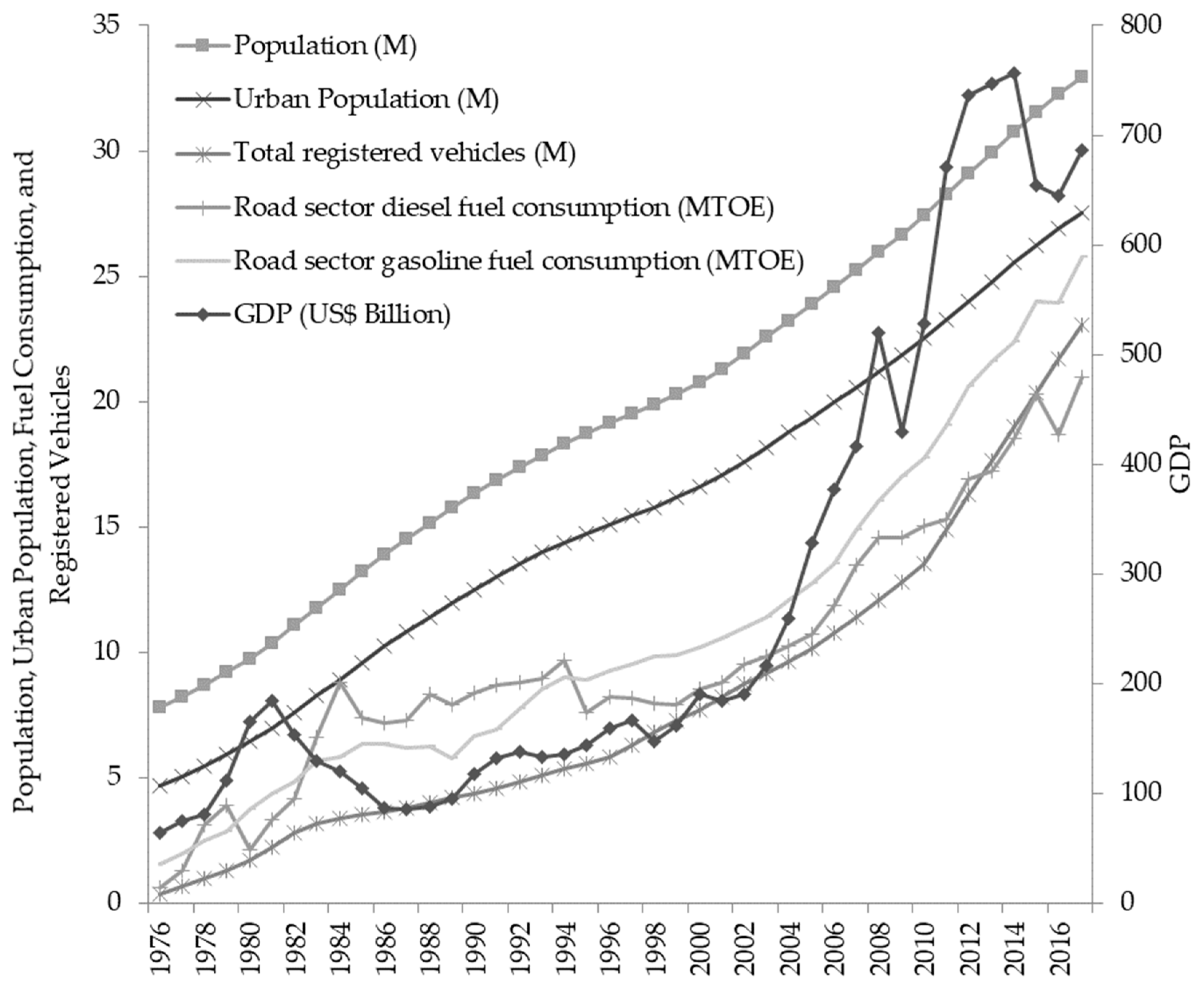
For forecasting energy demand, this study developed some AI-based energy demand models. We note that the accuracy of the energy demand-forecasting model is highly reliant on selected input variables. A high number of input variables may lead to overfitting and overtraining, resulting in reduced accuracy of models. Many socio-economic and demographic factors like GDP, population size, imports, exports, employment rate, and economic performance influence energy demand and forecasts. A country’s GDP is correlated with energy consumption. Some studies reveal that the most important elements of energy consumption are GDP, imports, exports, population size, fuel price, and the number of populations in urban agglomeration. Considered an indicator of a nation’s economic health, GDP measures overall economic activity. When GDP rises, people’s living standards rise along with them, leading to increased energy consumption. The amount of energy used is directly related to the number of people since more energy is used as the population grows. Hence, GDP, the number of registered vehicles, total population, fuel price, and the number of populations in urban agglomeration are input variables in this study. Figure 3 shows the trends of some of the variables for Saudi Arabia.

2.2. Causality Analysis Approach

Causality analysis based on the VECM has three major steps: unit root test, cointegration test, and short- and long-run Granger causality test. The current study aims to identify the critical drivers of road transport energy consumption, where energy consumption is the dependent variable, and socio-economic variables such as GDP, urban population, fuel price, and vehicle numbers are the explanatory variables. Therefore, the relationship between energy consumption and socio-economic variables can be represented as [3,40]:
Et = α + β1 GDPt + β2 Pt + β3 Ut + β4 Vt + εt
In the above equation, E, GDP, P, U, and V are road transport energy consumption, annual GDP, fuel price, urban population, and passenger vehicle number, respectively. The parameter α and t is intercept and year, respectively. The β1 to β4 are coefficients for GDP, P, U, and V, respectively, and εt is the constant error term.

2.2.1. Unit Root Test

One of the preconditions for using a VECM is that all variables need to be non-stationary at one level and stationary at their first differences. Therefore, the stationary test is crucial in a VECM, requiring a logarithmic form of the previous equation. The logarithmic form can be written as follows [3,40]:
ln(Et) = ln(α) + β1ln (GDPt) + β2 ln (Pt) + β3 ln (Ut) + β4 ln (Vt) + ln (εt)
The stationarity of the data set may be checked, and the integration sequence of the explanatory factors can be investigated using the Augmented Dickey–Fuller (ADF) and Phillips–Perron (PP) tests. The ADF test is used because it is considered to be the most widely used unit root test [42]. However, according to Azlina et al. [43], the ADF test often fails to reject a unit root. Therefore, this study used the PP and ADF tests for a robust result. The PP test is used because it is suitable mainly for small datasets, and this study has used a small length of time-series data from 1996 to 2017.

2.2.2. Co-Integration Test

Another precondition for developing a VECM is that at least two of the variables used in the study need to be co-integrated. Johansen’s cointegration test investigates the existence of cointegration among variables [44]. This test is used in this study because it is evident from the unit root test that all the variables are integrated in the same order, and the test performs better in such situations [45]. Thus, the Johansen cointegration test’s trace statistic and maximum Eigenvalue statistics are computed to examine the cointegration of the parameters. Trace and maximum Eigenvalue statistics are the two widely used statistics for identifying the number of co-integrating equations [10].

2.2.3. Granger Causality Test

Once it is evident that there is at least one co-integrating equation, a VECM can be developed, and the Granger causality test can be performed using that VECM framework [26]. The Granger causality test examines both the short- and long-term causality and provides the direction of causality. The error correction term (ECT) of a VECM indicates the adjustment speed towards attaining long-run equilibrium and helps to understand the long-run relationship and causality direction between the dependent and explanatory variables. The Wald F statistics of the Granger Causality test are for understanding the causal relationships and their directions among variables in the short run because this is the most widely used technique to explain short-run relationships [10].

2.3. Prediction Approach

The five main steps of the adopted methodology for future energy demand estimation include (i) input analysis, (ii) input projection, (iii) model construction, (iv) model testing, and (v) output (road transportation energy consumption in Saudi Arabia) forecasting:
Step
1: Input Processing—All the input data exhibit an increasing trend. Each variable’s linear trend is removed by developing a first-order linear regression model with the year as an input. A set of modified variables is obtained by eliminating the linear trend. In the next stage, normalization is performed to scale the data within the range between −1 and 1;
Step
2: Input Projection—A double exponential smoothing technique is employed to project the input data between 2018 and 2030;
Step
3: Model Development—The model is developed using the normalized input data between 1976 and 2004;
Step
4: Model Testing—The model is tested for the training data between 1976 and 2004 and the testing data between 2004 and 2017, considering suitable error measures;
Step
5: Output Forecasting—The model is utilized to make projections regarding the output. (road transport energy consumption in Saudi Arabia) for the period between 2018 and 2030 using the projected input data.

2.3.1. Double Exponential Smoothing

The analysis of the GDP, the number of registered vehicles, the total population, and the population in urban agglomeration data reveals a long-run trend. Double exponential smoothing is preferred over single exponential smoothing because it takes into account both the average and pattern. For n-periods-ahead prediction (Ft+n), the double exponential forecasting equation is as follows [46,47,48]:
Ft+n = Pt + nbt
where Pt is the projected intercept; bt is the projected slope. The equations are as follows [46,47,48]:
Pt = αyt + (1 − α) (Pt−1 + bt−1) for 0 ≤ α ≤ 1
bt = γ(PtPt−1) + (1 − γ) bt−1 for 0 ≤ γ ≤ 1
where [xt] represents the raw data sequence, α and γ are the data and trend smoothing factors, respectively. The selected initial values of P1 and b1 are equal to the observed value at t = 1 (i.e., x1) and the difference between the observed values at t = 2 and t = 1 (i.e., x2x1), respectively.

2.3.2. Support Vector Regression

The SVR was initially proposed by Cortes and Vapnik [49] on the basis of the structural risk minimization principle. The technique allows us to reduce the generalization error constraint without worrying too much about the training error. Generalization error is critical in evaluating the algorithm’s accuracy in forecasting unseen data. Although the applications of SVR were initially restricted to pattern recognition problems, the regression problems can also be solved now. The SVR builds an optimal geometric hyperplane for separating the data. It also uses nonlinear mapping ( ) to transform the data into a high-dimensional feature set before performing the linear regression in the transformed feature space [50,51,52].
For a mathematical explanation of the concept, let us consider x R n and y R , the hyper-plane function, y = f ( x ) = w . ( x ) + b , where w R n   = weight vector, and c R   = bias. The function ( x ) is a nonlinear transformation from R n to a higher dimensional space. Now, it is required to discover the w and b values for the determination of the x values by minimizing the regression risk [49,50,51,52]:
R = 1 2   i = 1 n { f ( x i ) y i } 2 + λ 2 w 2
where λ is the regularization constant, n indicates the sample inputs ( x 1 , . , x n ) , ( y 1 , . , y n ) refers to target output, and w represents the optimal desired weights vector of the regression hyperplane and can be represented as:
w * = i = 1 N ( β i β i * ) ( x i )
where β i , β i * are the solutions to the mentioned quadratic equation [51]. The regression equation can be rewritten by substituting w * :
f ( x , β , β * ) = i = 1 N ( β i β i * ) ( ( x i ) . ( x j ) + b = i = 1 n ( β i β i * ) K ( x i , x j ) + b
Here, K ( x i , x j ) is known as the kernel function, which is the product of the vectors x i and x j in the feature space. The considered kernel function can be a linear, polynomial, or radial basis function (RBF) and is written as:
K ( x i   , x j ) = e x p [ x i x j 2 2 σ 2 ]
where the user provides σ.
One common form of a cost function is Vapnik’s ε -insensitive loss function [53]:
E ε ( f ( x i ) y i ) = { | f ( x i ) y | ε ,     for   | f ( x i ) y | ε 0         Otherwise
Now, the quadratic problem is defined as:
Minimize   1 2 i = 1 n j = 1 n ( β i β i * ) ( β j β j * ) K ( x i , x j ) ε i = 1 n ( β i + β i * ) + i = 1 n ( β i β i * ) y i
Subject   to :   i = 1 n ( β i β i * ) = 0 ,   0 a n C ,   0 a n C
The β i   and   β i * are the forces which push and pull the estimate f ( x i ) towards the target output y i [54]. The constant C values cause penalties for errors in estimation for balancing the training error and generalization capability. The biases are determined using the Karush–Kuhn–Tucker (KKT) conditions [49,50,51,52].

2.3.3. Artificial Neural Networks

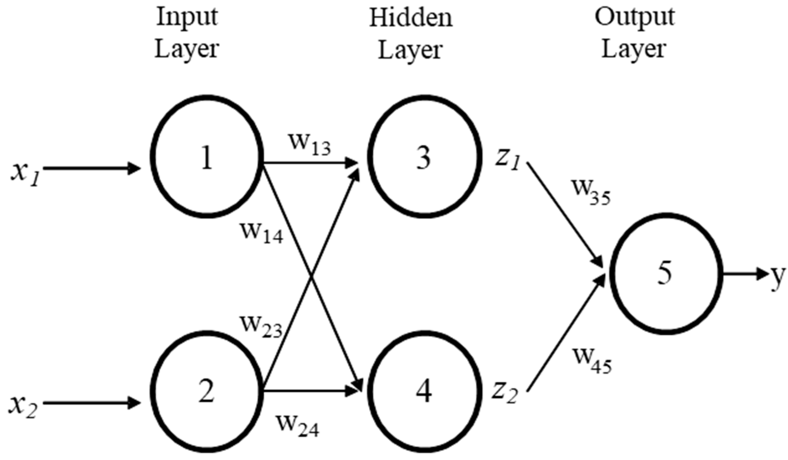
An ANN is a system of interconnected computing nodes (neurons). The information is processed similarly to how the human brain would. Multilayer perceptron (MLP) networks are the most popular type of neural networks. Each layer consists of neurons. Every neuron has a different weight associated with it. The information is passed from the input layer through hidden layers and finally reaches the output layer. Every neuron except the neuron in the input layer receives the information from the neurons in the preceding layer. After this, the neuron passes information to the output through a sigmoid function [55,56,57,58]. A training algorithm is adopted to obtain the weights while the algorithm minimizes the cost function, such as mean squared error considering the target and the model output. A general representation of a neural network is shown in Figure 4. As can be seen, the network consists of two inputs, one output, and one hidden layer. The input layer is not associated with any calculations; it simply transfers the input to the first hidden layer, while the remaining connections carry real-valued connection weights that modify the signal strength carried by other nodes. As inputs, the node of hidden layers and output layer receives the sum of the previous layer’s weighted outputs and the bias. The corresponding activation function modifies the input and transfers the result to the nodes of the subsequent layer or the environment.
The output of a node in the hidden layer and the output layer are in the following part as adopted from [55,56,57,58]. The output of the hidden node j:
z j = f ( q ) = e q e q + 1 ,   w h e r e   q = i w i j x i + w o j
where wij is the weight of the connection from the ith input node to the jth hidden node, and w0j is the bias of the jth hidden node. In the preceding example, the activation function of the hidden node is a sigmoid function with an input of q.
The final output can be represented as [56,57]:
y = w 35 z 1 + w 45 z 2
where w35 and w45 are the weights, and z1 and z2 are the output of the third and fourth nodes, respectively.

2.4. Model Development

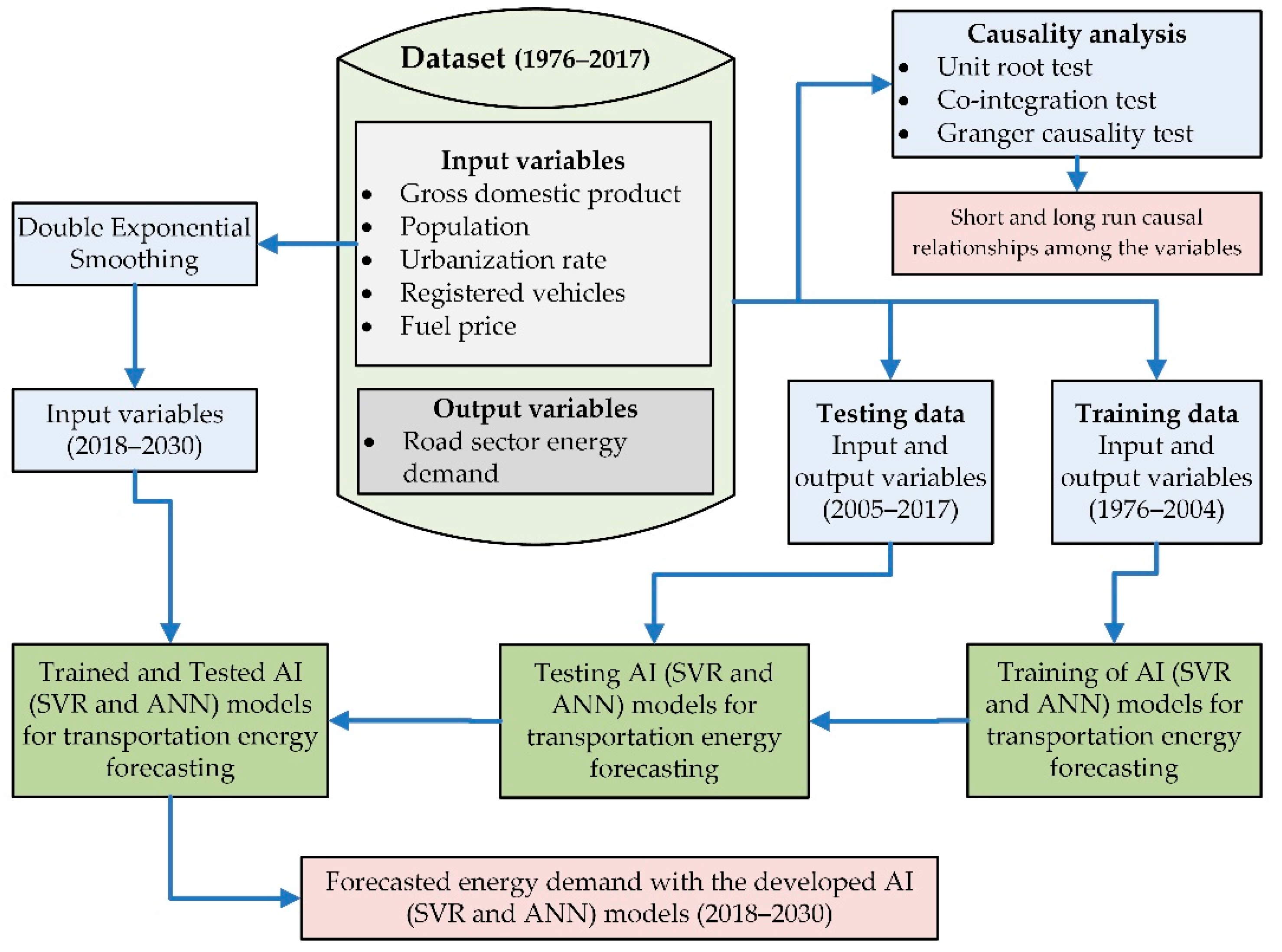
The ANN and SVR models were developed using MATLAB software. Data sets from 1976 to 2017 were used for analysis. Data from 1976–2004 were utilized for training, whereas data from 2005–2017 were used for testing. The data were projected up to 2030 using a double exponential smoothing technique. Data and trend smoothing factors were selected using the systematic trial and error process. Road transportation energy consumption was modeled using the projected input. Two important hyperparameters which need to be specified in the SVR model are appropriate C and ε values. With the goal of maintaining a balance between the learning error and the complexity of the model, C determines the optimal number of support vectors. The lower and higher C values are associated with underfitting and overfitting, respectively. When used to SVR, the ε is a normalization setting that establishes a compromise between error margin and model robustness to produce optimal adaptation on a new testing dataset. The smoothness of SVR’s response is affected by the value of ε. As a result, the model’s complexity and predictive validity rely on the parameter value of ε. After many systematic trial and error experiments, the values of C and ε are fixed to 1000 and 0.001, respectively. The conceptual framework of the suggested AI-model for predicting Saudi Arabia’s energy needs for road transport is depicted in Figure 5.
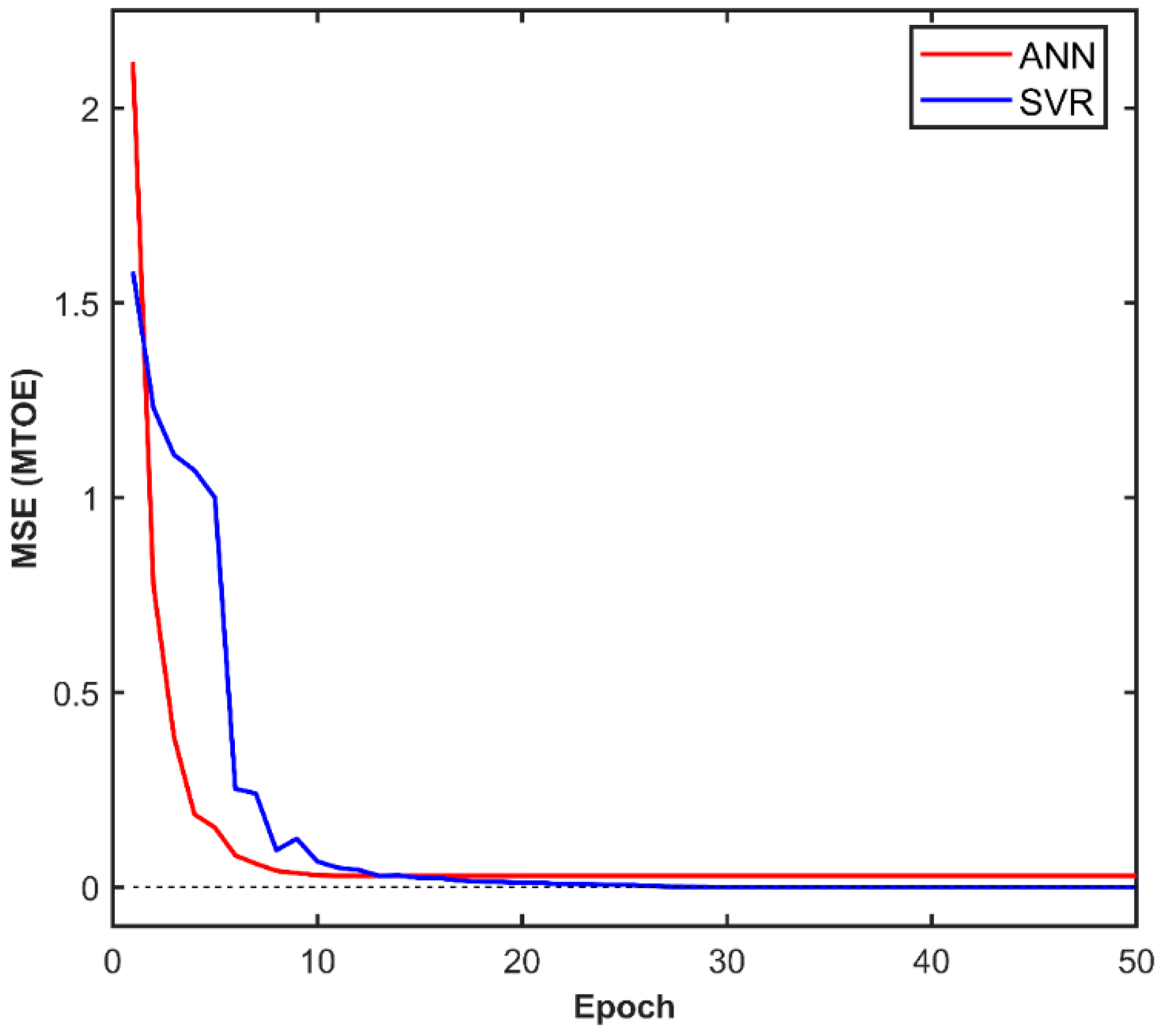
The important hyperparameters of an ANN include the number of hidden layers, the number of neurons in each layer, the learning algorithm, the activation function, the learning rate, and the learning goal. Due to the small dataset, only one hidden layer was considered in this study. The number of neurons in the hidden layer was ascertained through a systematic trial and error approach considering 1 to 4 neurons. The mean absolute percentage error values for the training dataset varied between 4.34% and 9.35% for the considered neurons. The testing results varied between 4.82% and 5.26% for the same number of neurons. The ANN with three neurons in the hidden layer with an activation function of tan-sigmoid, a learning rate of 0.00002, and a goal of 0.000001 produce the best result considering both the training and the testing results. Figure 6 presents the comparative analysis of ANN and SVR models in terms of mean squared error (MSE) index where the minimum values for the models were 0.0295 (MTOE) and 0.0001 (MTOE), respectively.

3. Results and Discussion

The section starts by demonstrating the results obtained from causality analysis approaches. Then, it presents the result of the developed SVR-based energy demand model along with different statistical performance measures to verify the efficacy of the developed model. Finally, a comparative analysis between the SVR-based and ANN-based approaches is also discussed.

3.1. Causality Analysis Model Results

In the unit root test, two specifications are used: the ‘intercept’ and the ‘Intercept and Trend.’ Table 1 presents the ADF and the PP test results for both specifications. All the variables are non-stationary at the level and stationary at their first differences, which is the first condition for developing a VECM for causality test analysis. The second condition for creating a VECM is the existence of cointegration between at least two of the variables. The Johansen cointegration test is performed to understand the cointegration among variables. The result is presented below in Table 2. The Johansen cointegration test result based on the Trace statistics and the Maximum Eigenvalue statistics shows that at least one co-integrating equation exists at a 1% significance level. The summary of the co-integrating equation is presented in Table 3. The signs of the coefficient values of the explanatory variables indicate that GDP and the number of vehicles have a positive relationship with transport energy consumption. In contrast, the relationship is negative between the urbanization rate and fuel prices. An increase in GDP or vehicle number increases transport energy consumption, while an increase in urbanization rate or fuel price decreases energy consumption. Since cointegration exists among variables and all the variables are non-stationary ‘at level’ and stationary ‘at their first differences’, a VECM has been developed to understand the long- and short-run causal relationship between transport energy consumption and its explanatory variables, as can be seen in Table 4.
The Granger causality test result shows that GDP and urbanization rate have short-run and long-run-causal relationships with transport energy consumption. However, the number of vehicles and fuel prices do not have a noteworthy causal relationship with energy consumption. Although vehicle number does not have a short-run causal relationship with fuel consumption, there is a causal relationship running from vehicle number to urban population rate and GDP. This means that policy measures are required to promote alternative modes of transportation, especially in urban areas. Since GDP has a strong causal relationship with transport energy consumption in the short and long run, energy intensity needs to be immediately reduced through appropriate policy measures. In addition, urbanization needs to be managed through high-density urban development instead of urban sprawl.

3.2. AI-Based Model Results

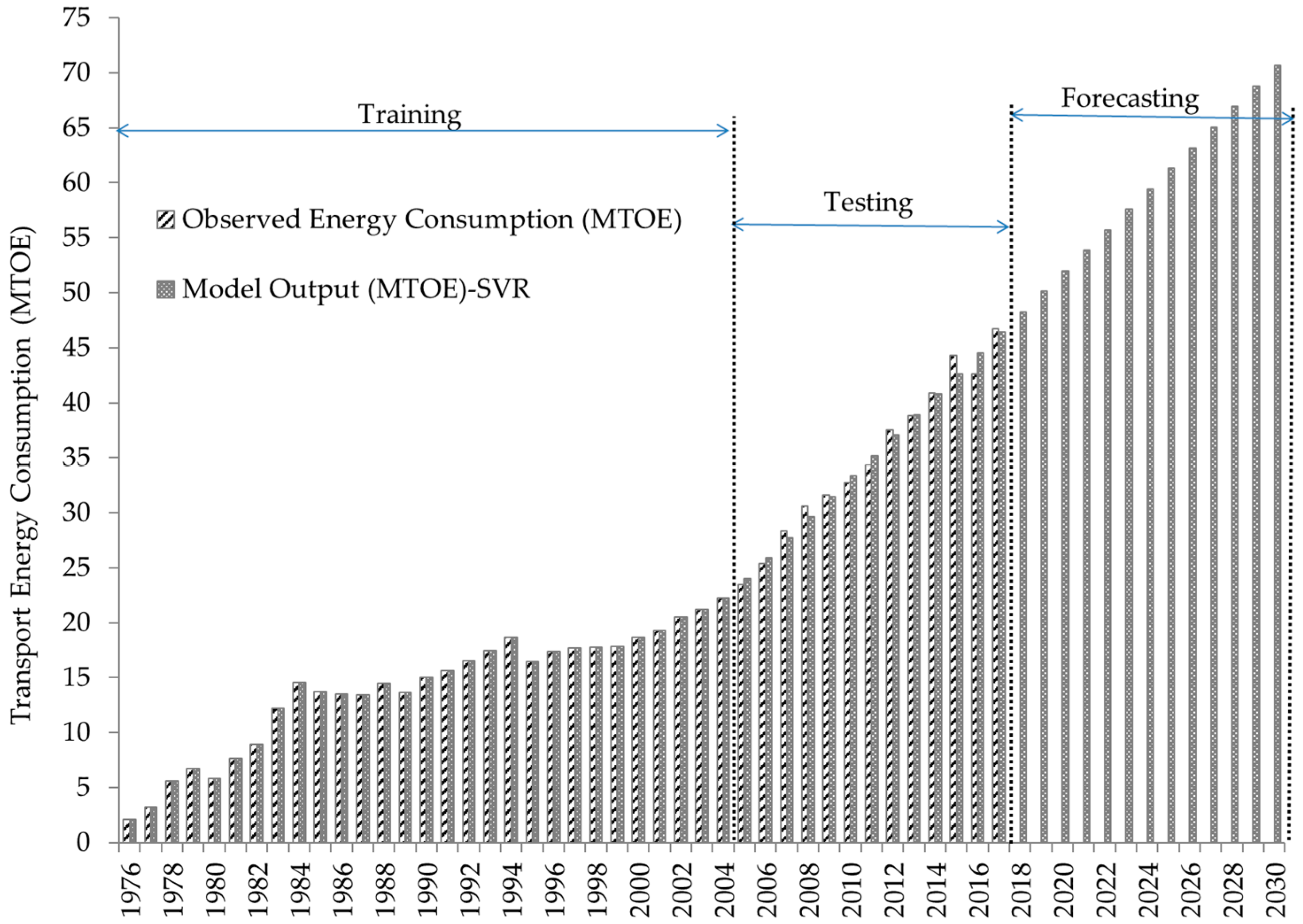
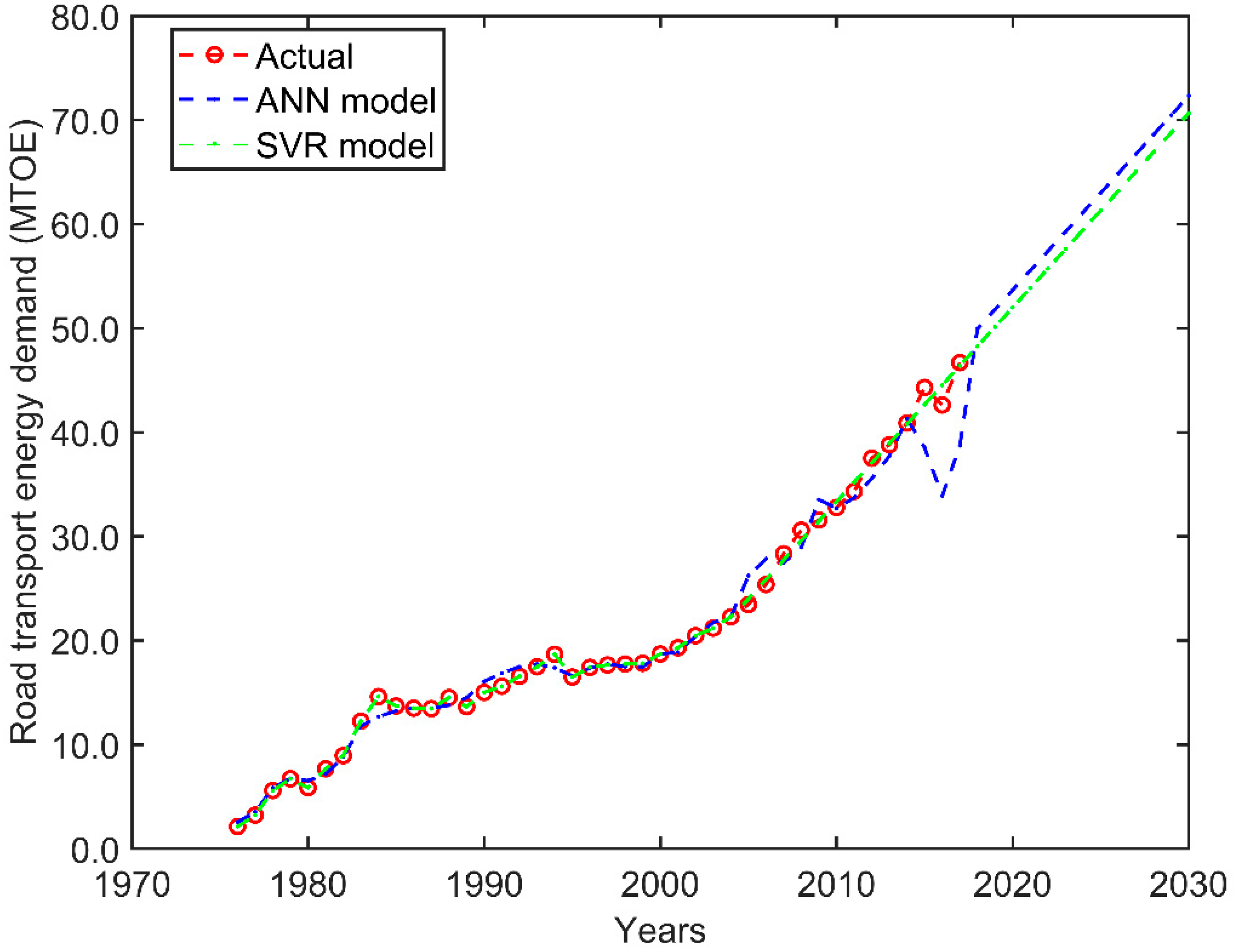
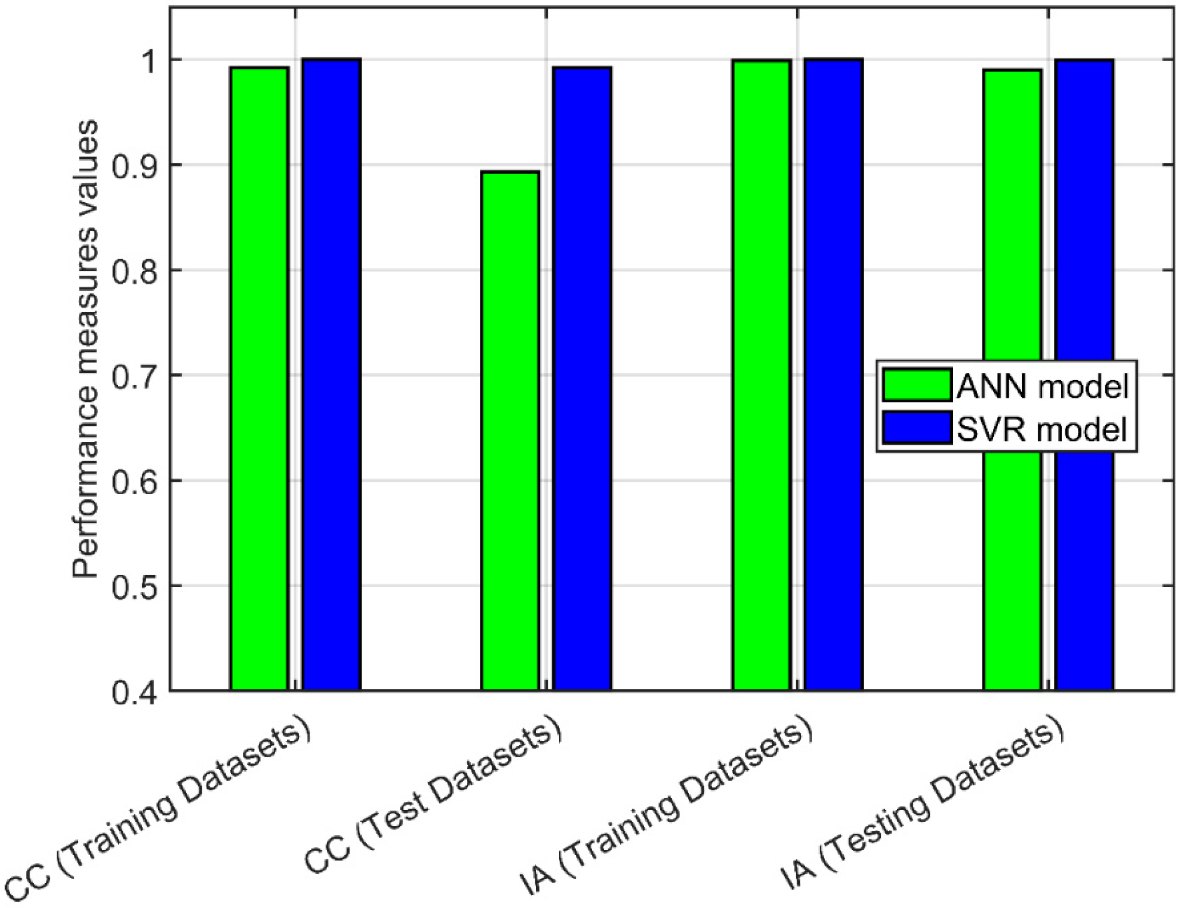
The input variables are forecasted to project the road transportation energy demand for Saudi Arabia between 2017 and 2030 (Figure 7 and Figure 8). Both the training (1976–2004) and testing (2005–2017) datasets are used to assess the created model’s efficacy. The model appears to produce results near the observed values for both training and testing datasets. Figure 9 presents the comparative illustrations of the machine learning models predicted energy demand for the road transportation sector of Saudi Arabia with actual energy demand. As can be seen, the SVR model predicted numbers are much closer to the actual numbers than ANN predicted numbers. Therefore, the superiority of the SVR model over the ANN model for the case under study (Saudi Arabia’s transportation sector energy prediction) is verified. The effectiveness of the model is assessed with the help of the root mean squared error (RMSE), mean absolute error (MAE), mean absolute percentage error (MAPE), correlation coefficient (CC), and Willmott’s index of agreement (IA). The values of IA for an ideal match and complete disagreement are 1 and 0, respectively [59]. The created model shows satisfactory performance on the training and testing datasets, as shown by the estimated values of the investigated performance measures (Table 5). The comparative analyses of the achieved performance indices for both machine-learning models are presented in Figure 10.
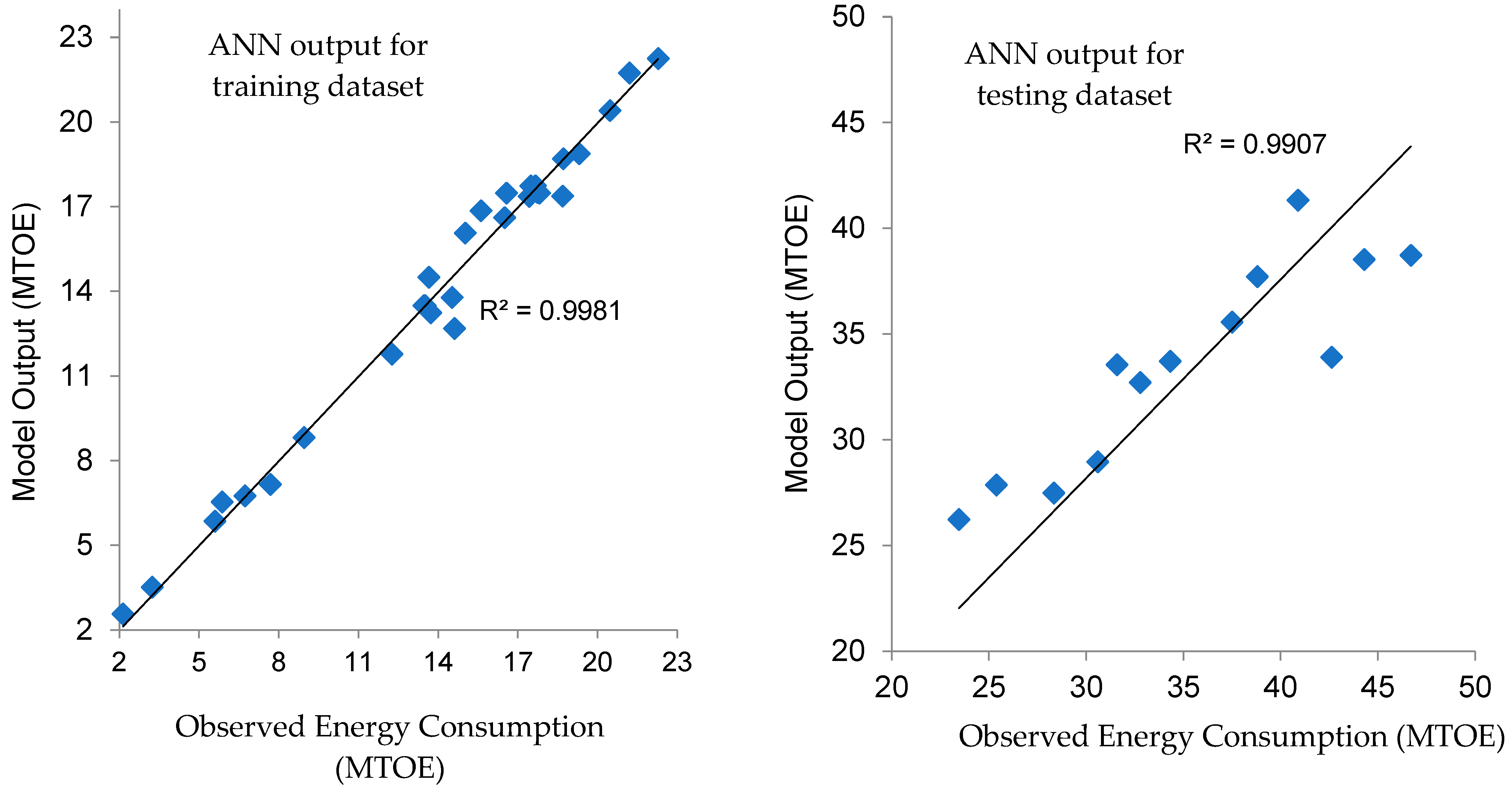
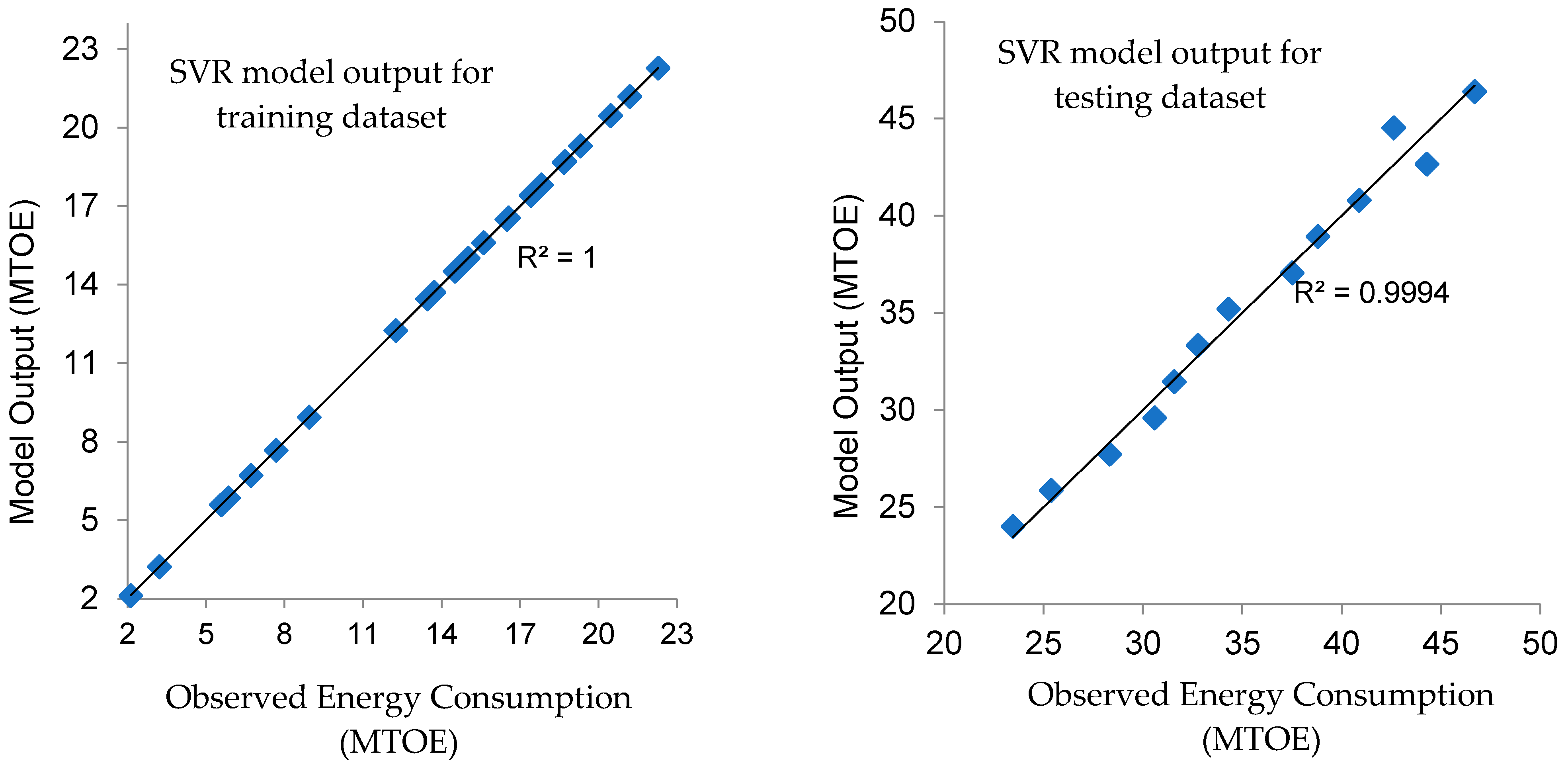
Figure 11 is a scatter plot illustrating the correlation between the data and the model’s predictions. An identity line, i.e., a y = x line, is generally drawn as the reference. The data points coincide with the identity line whenever the model’s predictions and observations are in perfect numerical agreement. For both the test and training datasets, the scatter diagram of the observable data and the model output showed that the prediction model reasonably conforms to the observed data. The coefficients of determination (R2) values are also satisfactory. Removing the trend line to concentrate on the nonlinear aspect of energy consumption and employing the twofold smoothing procedure for given input projection may account for the reliability of the observed data and the model’s predictions.

4. Conclusions and Policy Implementation

The rising energy usage of Saudi Arabia’s transport sector poses challenges to policymakers in achieving the country’s sustainability goals. As a result, the Kingdom must identify the factors that influence energy consumption trends in the sector and develop mitigation plans without compromising the country’s development. Considering the mentioned note, this article studied a few selected socio-economic drivers (GDP, fuel price, urban population, and passenger vehicle number) and their impacts on the energy trends of the sector using econometric analysis. Then, it predicted the future energy demand of the sector employing machine learning tools.
The econometric model analysis revealed that the GDP and urban population have short- and long-run causal relationships with road transport energy consumption. As of the co-integration test, the GDP affected energy consumption negatively, while urbanization affected it positively. Therefore, Saudi Arabia needs to shift its GDP growth towards a low-energy-intensive economy and manage its urban population growth tactfully to reduce both short-and long-run road transport energy demand. In addition, road transportation’s greenhouse gas emissions are directly proportionate to energy consumption because fossil fuels are the only source of energy in Saudi Arabia. Investments in renewables, public transport infrastructures, and low-carbon service sectors could be crucial to breaking the nexus between GDP, urbanization rate, and road transport energy consumption. In addition, promoting electric vehicles powered by renewables and fuel-efficient cars can be a valid option to reduce transport fuel consumption. Shift urban sprawl to smart growth to decouple the urban population from road transport energy consumption. Such a shift is likely to promote active travel (walking, cycling, etc.) and support public transport services, thereby reducing road transport energy consumption. These policy options are crucial for Saudi Arabia to tackle the critical drivers of energy demand in the transport sector and achieve environmental sustainability.
Prediction results of the future energy demand of road transportation employing machine learning models validated the efficacy of the SVR model over the ANN model. All selected statistical performance measures (RMSE, MAE, CC, and IA) for both training and testing datasets were better for the SVR model than the ANN model. For instance, the IA for the ANN model was 0.9899 for the testing dataset, whereas the value was only 0.9996 for the SVR model. Therefore, the concerned authorities can utilize the model for scenario development using different policy approaches to curtail road energy consumption. Although the overall performance of both machine learning models was adequate, both models did not realize the recent changes in energy demand well. Including additional relevant variables with longer time-series data can enhance the model performance. Moreover, other promising machine learning techniques including transparent machines, deep learning models, etc. can also be explored as an extension of this research to model energy demand of various sectors of the country.

Author Contributions

Conceptualization, S.M.R., M.A.H., U.G. and A.A.M.; methodology, S.M.R., M.A.H., M.S. and U.G.; software, S.M.R., M.A.H. and M.S.; validation, S.M.R., M.A.H., U.G., M.S., U.M., M.T.K. and A.A.M.; writing—original draft preparation, S.M.R., M.A.H., M.M.R., M.S. and O.R.; writing—review and editing, F.S.A.-I., S.M.R., M.A.H., U.G., M.S., U.M., M.T.K., O.R., M.M.R., A.A.M., M.A. and M.K.I.; supervision, S.M.R., M.A.H., F.S.A.-I., M.S. and M.M.R.; project administration, S.M.R., M.S. and M.A.H. All authors have read and agreed to the published version of the manuscript.

Funding

This research was funded by the Deanship of Scientific Research at King Faisal University (KFU), Al-Ahsa 31982, Saudi Arabia, through Project No. GRANT1517.

Institutional Review Board Statement

Not applicable.

Informed Consent Statement

Not applicable.

Data Availability Statement

The data that support the findings of this study are available from the corresponding author, M.M.R. ([email protected]), upon reasonable request.

Acknowledgments

The authors acknowledge the support received from the Deanship of Scientific Research at King Faisal University (KFU), King Fahd University of Petroleum & Minerals (KFUPM), and Al-Imam Mohammad Ibn Saud Islamic University, Saudi Arabia, University of Bahrain, and University of Utah, USA.

Conflicts of Interest

The authors declare no conflict of interest.

Appendix A

Table A1. Review of the energy demand estimation in the road transport sector.
Country and Ref. MethodologyModel DataForecasting PeriodPredicted
Variable
Predictor Variables
India by Bose et al. in 1997 [60] LEAP (Long-range Energy Alternatives Planning)1981–19891990–2010Passenger transport energy consumptionTotal number of vehicles, VMT (vehicles miles traveled), occupancy level, modal split, and fuel efficiency
Europe by Zachariadis et al. in 2003 [61] Macro-economic forecast1970–19992000–2030Transport energy demandGDP, population, VMT, occupancy rate, and fuel consumption
Nepal by Dhakal in 2003 [62] LEAP1998–20002005–2020Passenger transport energy consumptionTotal number of vehicles, annual vehicle kilometers traveled, occupancy level, and fuel efficiency
Turkey by Ozturk et al. in 2004 [19] Genetic algorithm1975–20022002–2020Energy demandPopulation, GDP, house production, export, and import
Turkey by Haldenbilen et al. in 2005 [22]Linear and quadratic equations using harmonic search1990–20002002–2020Energy demandPopulation, GDP, and VMT
Murat and Ceylan in 2006 [13]ANN1970–20012002–2020Energy demandGNP, population, annual average vehicle km, and historical energy data
Greece by Polemis in 2006 [63]Log-linear model1978–2003Not specifiedDiesel demandPer capita income and vehicle fleet, and gasoline and diesel prices
South Korea by Geem et al. in 2007 [64] ANN1980–2007Not specifiedEnergy demandGDP, import, export, and population
Turkey by Edigar et al. in 2007 [65] Autoregressive Integrated Moving Average (ARIMA)1950–20042005–2020Primary energy demandGDP, population, import, and export
Turkey by Sozen et al. in 2007 [66] ANN1968–2005Not specifiedNet energy demandGDP, population, import, and export
Turkey by Ceylan et al. in 2008 [67] Linear and quadratic equations using harmonic search1970–20052006–2025Road transport energy demandPopulation, GDP, and VMT
China by Yan et al. in 2009 [68]LEAP2000–20052005–2030Road transport energy demandTotal number of vehicles, VMT, and fuel economy
Taiwan by Lu et al. in 2009 [69]Grey forecasting model1990–20062007–2025Road transport energy demandPopulation, GDP, and VMT
Pakistan by Shabbir et al. in 2010 [70]LEAP20002000–2030 Urban passenger transport energy consumptionTotal number of vehicles, VMT, occupancy level, modal split, and fuel efficiency
Iran by Behrang et al. in 2011 [71] Bee algorithm1981–20052006–2030Energy demandpopulation, GDP, export, and import
South Korea by Geem in 2011 [14]ANN1990–20072008–2025Energy demandGDP, population, passenger transport amount, number of vehicle registrations, and oil price
Jordan by AhmedAl-Ghandoor et al. in 2012 [72]Adaptive neuro-fuzzy inference system (ANFIS)1985–20092010–2030Energy demandvehicles no./year, vehicle ownership and income level, and fuel price
Croatia by Pukšec et al. in 2013 [73]Energy demand of transport (EDT) modelNot specified2008–2050Long-term energy demandRailway, road, seawater and coastal, inland waterway, and air transports
Iran by Sadri et al. in 2014 [74]LEAP and EnergyPLAN1997–20082009–2025Long-term energy demandGDP and population
United States by Kialashaki and Reisel in 2014 [75]ANN and multiple linear regression1981–20092010–2030Energy demandGDP, population, oil price, and vehicles
Thailand by Tansawat et al. in 2015 [76]Linear and log-linear regression models2007Not specifiedTransport fuel consumptionGross provincial product, total number of sedans and gas stations, and a few dummy variables
Malaysia by Azam et al. in 2016 [77]LEAP1990–20122013–2040Long-term energy demandHistorical data
China by Chai et al. in 2016 [78]ARIMA and ETS (Error, Trend, Seasonal) models1971–20112012–2020Energy demandGDP, employment, urbanization rate, core business tax, total road turnover, highway mileage, car manufacturing charges, and automobile industry output
Saudi Arabia by Alshehry and Belloumia in 2017 [79]Environmental Kuznets curve 1971–2011Not specifiedTransport CO2 emissionsGDP, transport CO2 emissions, and transport energy consumption
China by Teng et al. in 2017 [80]Group method of data handling1980–20112012–2052Long-term energy demandGDP, population, urbanization rate, incomes, passenger, and freight turnovers, registered vehicle numbers, and fuel retail price index
24 countries in the Latin America by Llorca et al. in 2017 [81]Stochastic frontier approach1990–2010Not specifiedEnergy demandGDP, population, energy price index, gross value added, and population density
China by Peng et al. in 2018 [82]CPREG model20152015–2050Energy demand and GHG emissionsGDP, population, vehicle miles traveled, and vehicle stock
New Zealand by Hasan et al. in 2019 [10]Regression1990–20162017–2030Emissions from the road transport sectorDemography and urban economics, energy, socio-economic development transport factors, and politics and policies
Indonesia by Deendarlianto et al. in 2020 [83]Sustainable mobility project (SMP) model1999 –20132014–2030Energy demandGDP, population, vehicle type, travel distance, and fuel economy
Turkey by Talebi et al. in 2021 [84]ANN1975–20162020–2030Energy demandGDP, population, oil prices, ton-km, vehicle-km, and passenger-km
Taiwan by Yao et al. in 2021 [85]Convolutional neural network1999–2019Up to 2025Energy demandGDP, population, number of registered vehicles, passenger transport value, and oil price
Turkey by Sahraei et al. in 2021 [86]Multivariate adaptive regression splines1975–20192020–2030Energy demandGDP, population, oil price, vehicle-km, passenger-km, and ton-km
Malaysia by Solaymani in 2022 [87]Autoregressive distributed lag (ARDL)1978–2018Not specifiedCO2 emissions GDP, urbanization, energy and carbon intensity, and renewable energy in energy mix.
Turkey by Turgut et al. in 2021 [88]OPTSGULL algorithm 1970–20172018–2028Energy demandGDP, population, employment, trade, inflation, crude oil price, total amount of goods transported, and total vehicle travel in km
Turkey by Özdemiïr and Dörterler in 2022 [89]Linear, exponential, and quadratic models assisted by heuristic algorithm1970–20132014–2034Energy demandGDP, total vehicle kilometer/year, population
Morocco Oubnaki et al. in 2022 [90]Regression models1990–20142020–2030Energy demandGDP, population, urbanization, fuel price, working women rate, number of vehicles registration and active vehicles on the road, and activity rate by gender and category
28 European countries by Maaouane et al. in 2022 [91]ANN1990–20192020–2050Energy demandGDP, population, population density, gasoline and diesel price, purchasing power parity, price index, and household final consumption expenditure
Turkey by Sahraei and Çodur in 2022 [86]Hybrid meta-heuristic ANN1975–2019 (First 80%)1975–2019 (Last 20%)Energy demandGDP, population, oil price, passenger-km, vehicle-km, and ton-km
Pakistan by Asim et al. in 2022 [92]LEAP2003–20182019–2035Energy consumptionHistorical energy consumption data

References

  1. Shah, I.; Iftikhar, H.; Ali, S. Modeling and Forecasting Electricity Demand and Prices: A Comparison of Alternative Approaches. J. Math. 2022, 2022, 3581037. [Google Scholar] [CrossRef]
  2. Nan, R.; Xu, H. The Relationship between Energy Consumption and Economic Growth Based on Vector Error Correction Model. Chem. Eng. Trans. 2018, 67, 817–822. [Google Scholar]
  3. Rahman, M.M.; Hasan, M.A.; Shafiullah, M.; Rahman, M.S.; Arifuzzaman, M.; Islam, M.K.; Islam, M.M.; Rahman, S.M. A Critical, Temporal Analysis of Saudi Arabia’s Initiatives for Greenhouse Gas Emissions Reduction in the Energy Sector. Sustainability 2022, 14, 12651. [Google Scholar] [CrossRef]
  4. Fonseca, J.; Vieira, M.; Madeira, H. Training Security Assurance Teams Using Vulnerability Injection. In Proceedings of the 14th IEEE Pacific Rim International Symposium on Dependable Computing, Taipei, Taiwan, 15–17 December 2008; IEEE: Piscataway, NJ, USA, 2008; pp. 297–304. [Google Scholar]
  5. Porteiro, R.; Hernández-Callejo, L.; Nesmachnow, S. Electricity Demand Forecasting in Industrial and Residential Facilities Using Ensemble Machine Learning. Rev. Fac. Ing. 2022, 102, 9–25. [Google Scholar] [CrossRef]
  6. Rahman, S.M.; Al-Ismail, F.S.; Haque, M.E.; Shafiullah, M.; Islam, M.R.; Chowdhury, M.T.; Alam, M.S.; Razzak, S.A.; Ali, A.; Khan, Z.A. Electricity Generation in Saudi Arabia: Tracing Opportunities and Challenges to Reducing Greenhouse Gas Emissions. IEEE Access 2021, 9, 116163–116182. [Google Scholar] [CrossRef]
  7. Trewin, D. Year Book, Australia 2001. Available online: https://archive.org/stream/australianyearbook20011/Australian_Yearbook_2001-3_djvu.txt (accessed on 14 September 2022).
  8. World Atlas The 15 Richest Countries In The World—WorldAtlas. Available online: https://www.worldatlas.com/articles/the-richest-countries-in-the-world.html (accessed on 14 September 2022).
  9. Central Intelligence Agency of USA The World Factbook. Available online: https://www.cia.gov/the-world-factbook/about/cover-gallery/2017-cover/ (accessed on 14 September 2022).
  10. Hasan, M.A.; Frame, D.J.; Chapman, R.; Archie, K.M. Emissions from the Road Transport Sector of New Zealand: Key Drivers and Challenges. Environ. Sci. Pollut. Res. 2019, 26, 23937–23957. [Google Scholar] [CrossRef]
  11. Lee, C.; Chang, C. The Impact of Energy Consumption on Economic Growth: Evidence from Linear and Nonlinear Models in Taiwan. Energy 2007, 32, 2282–2294. [Google Scholar] [CrossRef]
  12. Haldenbilen, S.; Ceylan, H. Genetic Algorithm Approach to Estimate Transport Energy Demand in Turkey. Energy Policy 2005, 33, 89–98. [Google Scholar] [CrossRef]
  13. Murat, Y.S.; Ceylan, H. Use of Artificial Neural Networks for Transport Energy Demand Modeling. Energy Policy 2006, 34, 3165–3172. [Google Scholar] [CrossRef]
  14. Geem, Z.W. Transport Energy Demand Modeling of South Korea Using Artificial Neural Network. Energy Policy 2011, 39, 4644–4650. [Google Scholar] [CrossRef]
  15. Zhang, M.; Mu, H.; Li, G.; Ning, Y. Forecasting the Transport Energy Demand Based on PLSR Method in China. Energy 2009, 34, 1396–1400. [Google Scholar] [CrossRef]
  16. Kankal, M.; Akpınar, A.; Kömürcü, M.İ.; Özşahin, T.Ş. Modeling and Forecasting of Turkey’s Energy Consumption Using Socio-Economic and Demographic Variables. Appl. Energy 2011, 88, 1927–1939. [Google Scholar] [CrossRef]
  17. Limanond, T.; Jomnonkwao, S.; Srikaew, A. Projection of Future Transport Energy Demand of Thailand. Energy Policy 2011, 39, 2754–2763. [Google Scholar] [CrossRef]
  18. Soytas, U.; Sari, R. Energy Consumption and GDP: Causality Relationship in G-7 Countries and Emerging Markets. Energy Econ. 2003, 25, 33–37. [Google Scholar] [CrossRef]
  19. Ozturk, H.; Canyurt, O.; Hepbasli, A.; Utlu, Z. Residential-Commercial Energy Input Estimation Based on Genetic Algorithm (GA) Approaches: An Application of Turkey. Energy Build. 2004, 36, 175–183. [Google Scholar] [CrossRef]
  20. Canyurt, O.E.; Ceylan, H.; Ozturk, H.K.; Hepbasli, A. Energy Demand Estimation Based on Two-Different Genetic Algorithm Approaches. Energy Sources 2004, 26, 1313–1320. [Google Scholar] [CrossRef]
  21. Azadeh, A.; Ghaderi, S.; Sohrabkhani, S. Annual Electricity Consumption Forecasting by Neural Network in High Energy Consuming Industrial Sectors. Energy Convers. Manag. 2008, 49, 2272–2278. [Google Scholar] [CrossRef]
  22. An, N.; Zhao, W.; Wang, J.; Shang, D.; Zhao, E. Using Multi-Output Feedforward Neural Network with Empirical Mode Decomposition Based Signal Filtering for Electricity Demand Forecasting. Energy 2013, 49, 279–288. [Google Scholar] [CrossRef]
  23. Uzlu, E.; Kankal, M.; Akpınar, A.; Dede, T. Estimates of Energy Consumption in Turkey Using Neural Networks with the Teaching–Learning-Based Optimization Algorithm. Energy 2014, 75, 295–303. [Google Scholar] [CrossRef]
  24. Deshani, K.; Hansen, L.; Attygalle, M.D.T.; Karunarathne, A. Improved Neural Network Prediction Performances of Electricity Demand: Modifying Inputs through Clustering. In Proceedings of the Second International Conference on Computational Science and Engineering, Coimbatore, India, 26–28 October 2012; pp. 137–147. [Google Scholar]
  25. Li, Q.; Meng, Q.; Cai, J.; Yoshino, H.; Mochida, A. Applying Support Vector Machine to Predict Hourly Cooling Load in the Building. Appl. Energy 2009, 86, 2249–2256. [Google Scholar] [CrossRef]
  26. Jiang, Y.; Zhao, Q.; Lu, Y. Ensemble Based Data Stream Mining with Recalling and Forgetting Mechanisms. In Proceedings of the 11th International Conference on Fuzzy Systems and Knowledge Discovery (FSKD), Xiamen, China, 19–21 August 2014; IEEE: Piscataway, NJ, USA, 2014; pp. 430–435. [Google Scholar]
  27. Liao, S.; Chu, P.; Hsiao, P. Data Mining Techniques and Applications–A Decade Review from 2000 to 2011. Expert Syst. Appl. 2012, 39, 11303–11311. [Google Scholar] [CrossRef]
  28. Hong, W. Hybrid Evolutionary Algorithms in a SVR-Based Electric Load Forecasting Model. Electr. Power Energy Syst. 2009, 31, 409–417. [Google Scholar] [CrossRef]
  29. Shafiullah, M.; Abido, M.A.; Al-Mohammed, A.H. Power System Fault Diagnosis: A Wide Area Measurement Based Intelligent Approach, 1st ed.; Elsevier: Amsterdam, The Netherlands, 2022; ISBN 9780323884303. [Google Scholar]
  30. Jain, R.; Smith, K.M.; Culligan, P.J.; Taylor, J.E.; Jain, R.K.; Taylor, J.E. Forecasting Energy Consumption of Multi-Family Residential Buildings Using Support Vector Regression: Investigating the Impact of Temporal and Spatial Monitoring. Appl. Energy 2014, 123, 168–178. [Google Scholar] [CrossRef]
  31. Kavousi-Fard, A.; Samet, H.; Marzbani, F. A New Hybrid Modified Firefly Algorithm and Support Vector Regression Model for Accurate Short Term Load Forecasting. Expert Syst. Appl. 2014, 41, 6047–6056. [Google Scholar] [CrossRef]
  32. Omid, M.; Khoshnevisan, B.; Ramedani, Z.; Keyhani, A.; Shamshirband, S. Potential of Radial Basis Function Based Support Vector Regression for Global Solar Radiation Prediction. Energy Rev. 2014, 39, 1005–1011. [Google Scholar] [CrossRef]
  33. Chia, Y.; Lee, L.; Shafiabady, N.; Isa, D. A Load Predictive Energy Management System for Supercapacitor-Battery Hybrid Energy Storage System in Solar Application Using the Support Vector Machine. Appl. Energy 2015, 137, 588–602. [Google Scholar] [CrossRef]
  34. Fu, R. An Improved Support Vector Machine Algorithm and Its Application in Intelligent Transportation System. Chem. Eng. Trans. 2016, 51, 601–606. [Google Scholar]
  35. Jamal, A.; Reza, I.; Shafiullah, M. Modeling Retroreflectivity Degradation of Traffic Signs Using Artificial Neural Networks. IATSS Res. 2022, in press. [Google Scholar] [CrossRef]
  36. Meng, M.; Toan, T.D.; Wong, Y.D.; Lam, S.H. Short-Term Travel-Time Prediction Using Support Vector Machine and Nearest Neighbor Method. Transp. Res. Rec. J. Transp. Res. Board 2022, 2676, 353–365. [Google Scholar] [CrossRef]
  37. Ullah, I.; Liu, K.; Yamamoto, T.; Shafiullah, M.; Jamal, A. Grey Wolf Optimizer-Based Machine Learning Algorithm to Predict Electric Vehicle Charging Duration Time. Transp. Lett. 2022, 15, 1–18. [Google Scholar] [CrossRef]
  38. Zou, Y.; Hua, X.; Zhang, Y.; Wang, Y. Hybrid Short-Term Freeway Speed Prediction Methods Based on Periodic Analysis. Can. J. Civ. Eng. 2015, 42, 570–582. [Google Scholar] [CrossRef]
  39. Sun, J.; Sun, J.; Chen, P. Use of Support Vector Machine Models for Real-Time Prediction of Crash Risk on Urban Expressways. Transp. Res. Rec. J. Transp. Res. Board 2014, 2432, 91–98. [Google Scholar] [CrossRef]
  40. Rahman, M.M.; Rahman, S.M.; Rahman, M.S.; Hasan, A.; Shoaib, S.A.; Rushd, S. Greenhouse Gas Emissions from Solid Waste Management in Saudi Arabia—Analysis of Growth Dynamics and Mitigation Opportunities. Appl. Sci. 2021, 11, 1737. [Google Scholar] [CrossRef]
  41. The World Bank. World Development Indicators DataBank. Available online: https://databank.worldbank.org/source/world-development-indicators (accessed on 16 September 2022).
  42. Fedorova, D. Selection of Unit Root Test on the Basis of Length of the Time Series and Value of Ar (1) Parameter. Statistika 2016, 96, 3. [Google Scholar]
  43. Azlina, A.; Law, S.; Mustapha, N. Dynamic Linkages among Transport Energy Consumption, Income and CO2 Emission in Malaysia. Energy Policy 2014, 73, 598–606. [Google Scholar] [CrossRef]
  44. Johansen, S.; Juselius, K. Maximum Likelihood Estimation and Inference on Cointegration—With Appucations to the Demand for Money. Oxf. Bull. Econ. Stat. 1990, 52, 169–210. [Google Scholar] [CrossRef]
  45. Güzel, A.E.; Arslan, Ü. On the Nexus between Exchange Rate and Income Distribution in Turkey: ARDL Bound Testing Analysis. Econ. J. Emerg. Mark. 2019, 11, 1–7. [Google Scholar] [CrossRef] [Green Version]
  46. Sullivan, W.G.; Claycombe, W.W. Fundamentals of Forecasting, 1st ed.; Reston Pub. Co.: Reston, VA, USA, 1977; ISBN 978-0879093006. [Google Scholar]
  47. Lukman, M.; Tanan, B.; Khairina, D.M.; Daniel, Y.; Widagdo, P.P.; Sidqi, F.; Sumitra, I.D. Forecasting Product Selling Using Single Exponential Smoothing and Double Exponential Smoothing Methods. IOP Conf. Ser. Mater. Sci. Eng. 2019, 662, 032031. [Google Scholar] [CrossRef]
  48. Adamuthe, A.C.; Gage, R.A.; Thampi, G.T. Forecasting Cloud Computing Using Double Exponential Smoothing Methods. In Proceedings of the ICACCS 2015—2nd International Conference on Advanced Computing and Communication Systems, Coimbatore, India, 5–7 January 2015. [Google Scholar] [CrossRef]
  49. Cortes, C.; Vapnik, V.; Saitta, L. Support-Vector Networks. Mach. Learn. 1995, 20, 273–297. [Google Scholar] [CrossRef]
  50. Boser, B.E.; Guyon, I.M.; Vapnik, V.N. A Training Algorithm for Optimal Margin Classifiers. In Proceedings of the Fifth Annual ACM Workshop on Computational Learning Theory, Pittsburgh, PA, USA, 27–29 July 1992; ACM: New York, NY, USA, 1992; pp. 144–152. [Google Scholar]
  51. Vapnik, V. The Nature of Statistical Learning Theory; Springer: New York, NY, USA, 1995. [Google Scholar]
  52. Shafiullah, M.; Abido, M.A.; Al-Mohammed, A.H. Artificial Intelligence Techniques. In Power System Fault Diagnosis; Elsevier: Cambridge, MA, USA, 2022; Chapter 3; pp. 69–100. [Google Scholar] [CrossRef]
  53. Smola, A.J.; Schölkopf, B. A Tutorial on Support Vector Regression. Stat. Comput. 2004, 14, 199–222. [Google Scholar] [CrossRef] [Green Version]
  54. Burges, C.J.C. A Tutorial on Support Vector Machines for Pattern Recognition. Data Min. Knowl. Discov. 1998, 2, 121–167. [Google Scholar] [CrossRef]
  55. Usman, M.; Hussain, H.; Riaz, F.; Irshad, M.; Bashir, R.; Shah, M.H.; Zafar, A.A.; Bashir, U.; Kalam, M.A.; Mujtaba, M.A.; et al. Artificial Neural Network Led Optimization of Oxyhydrogen Hybridized Diesel Operated Engine. Sustainability 2021, 13, 9373. [Google Scholar] [CrossRef]
  56. Shahriar, M.S.; Shafiullah, M.; Rana, M.J.; Ali, A.; Ahmed, A.; Rahman, S.M. Neurogenetic Approach for Real-Time Damping of Low-Frequency Oscillations in Electric Networks. Comput. Electr. Eng. 2020, 83, 106600. [Google Scholar] [CrossRef]
  57. Shafiullah, M.; Abido, M.A.; Al-Mohammed, A.H. Intelligent Fault Diagnosis for Distribution Grid Considering Renewable Energy Intermittency. Neural Comput. Appl. 2022, 34, 16473–16492. [Google Scholar] [CrossRef]
  58. Ahmed, E.; Usman, M.; Anwar, S.; Ahmad, H.M.; Nasir, M.W.; Malik, M.A.I. Application of ANN to Predict Performance and Emissions of SI Engine Using Gasoline-Methanol Blends. Sci. Prog. 2021, 104, 00368504211002345. [Google Scholar] [CrossRef]
  59. Willmott, C.J. On the Validation of Models. Phys. Geogr. 1981, 2, 184–194. [Google Scholar] [CrossRef]
  60. Bose, R.; Srinivasachary, V. Policies to Reduce Energy Use and Environmental Emissions in the Transport Sector: A Case of Delhi City. Energy Policy 1997, 25, 1137–1150. [Google Scholar] [CrossRef]
  61. Zachariadis, T.; Kouvaritakis, N. Long-Term Outlook of Energy Use and CO2 Emissions from Transport in Central and Eastern Europe. Energy Policy 2003, 31, 759–773. [Google Scholar] [CrossRef]
  62. Dhakal, S. Implications of Transportation Policies on Energy and Environment in Kathmandu Valley, Nepal. Energy Policy 2003, 31, 1493–1507. [Google Scholar] [CrossRef]
  63. Polemis, M. Empirical Assessment of the Determinants of Road Energy Demand in Greece. Energy Econ. 2006, 28, 385–403. [Google Scholar] [CrossRef]
  64. Geem, Z.; Roper, W. Energy Demand Estimation of South Korea Using Artificial Neural Network. Energy Policy 2009, 37, 4049–4054. [Google Scholar] [CrossRef]
  65. Ediger, V.; Akar, S. ARIMA Forecasting of Primary Energy Demand by Fuel in Turkey. Energy Policy 2007, 35, 1701–1708. [Google Scholar] [CrossRef]
  66. Sözen, A.; Arcaklioglu, E. Prediction of Net Energy Consumption Based on Economic Indicators (GNP and GDP) in Turkey. Energy Policy 2007, 35, 4981–4992. [Google Scholar] [CrossRef]
  67. Ceylan, H.; Ceylan, H.; Haldenbilen, S.; Baskan, O. Transport Energy Modeling with Meta-Heuristic Harmony Search Algorithm, an Application to Turkey. Energy Policy 2008, 36, 2527–2535. [Google Scholar] [CrossRef]
  68. Yan, X.; Crookes, R. Reduction Potentials of Energy Demand and GHG Emissions in China’s Road Transport Sector. Energy Policy 2009, 37, 658–668. [Google Scholar] [CrossRef]
  69. Lu, I.; Lewis, C.; Lin, S. The Forecast of Motor Vehicle, Energy Demand and CO2 Emission from Taiwan’s Road Transportation Sector. Energy Policy 2009, 37, 2952–2961. [Google Scholar] [CrossRef]
  70. Shabbir, R.; Ahmad, S. Monitoring Urban Transport Air Pollution and Energy Demand in Rawalpindi and Islamabad Using Leap Model. Energy 2010, 35, 2323–2332. [Google Scholar] [CrossRef]
  71. Behrang, M.A.; Assareh, E.; Assari, M.R.; Ghanbarzadeh, A. Total Energy Demand Estimation in Iran Using Bees Algorithm. Energy Sources Part B Econ. Plan. Policy 2011, 6, 294–303. [Google Scholar] [CrossRef]
  72. Al-Ghandoor, A.; Samhouri, M.; Al-Hinti, I.; Jaber, J.; Al-Rawashdeh, M. Projection of Future Transport Energy Demand of Jordan Using Adaptive Neuro-Fuzzy Technique. Energy 2012, 38, 128–135. [Google Scholar] [CrossRef]
  73. Pukšec, T.; Krajačić, G.; Lulić, Z.; Mathiesen, B.V.; Duić, N. Forecasting Long-Term Energy Demand of Croatian Transport Sector. Energy 2013, 57, 169–176. [Google Scholar] [CrossRef] [Green Version]
  74. Sadri, A.; Ardehali, M.M.; Amirnekooei, K. General Procedure for Long-Term Energy-Environmental Planning for Transportation Sector of Developing Countries with Limited Data Based on LEAP (Long-Range Energy Alternative Planning) and EnergyPLAN. Energy 2014, 77, 831–843. [Google Scholar] [CrossRef]
  75. Kialashaki, A.; Reisel, J. Transport Energy Demand Modeling of the United States Using Artificial Neural Networks and Multiple Linear Regressions. In Proceedings of the ASME 2014 8th International Conference on Energy Sustainability collocated with the ASME 2014 12th International Conference on Fuel Cell Science, Engineering and Technology, Boston, MA, USA, 30 June–2 July 2014; Volume 2. [Google Scholar] [CrossRef]
  76. Tansawat, T.; Pochan, J.; Mofadal, A. Transport Energy Consumption Model for Thailand Provinces. In Proceedings of the 5th Atrans Symposium Student Chapter Session, Bangkok, Thailand, 24–25 August 2012; pp. 187–195. [Google Scholar]
  77. Azam, M.; Othman, J.; Begum, R.A.; Abdullah, S.M.S.; Nor, N.G.M. Energy Consumption and Emission Projection for the Road Transport Sector in Malaysia: An Application of the LEAP Model. Environ. Dev. Sustain. 2016, 18, 1027–1047. [Google Scholar] [CrossRef]
  78. Chai, J.; Lu, Q.Y.; Wang, S.Y.; Lai, K.K. Analysis of Road Transportation Energy Consumption Demand in China. Transp. Res. Part D Transp. Environ. 2016, 48, 112–124. [Google Scholar] [CrossRef]
  79. Alshehry, A.S.; Belloumi, M. Study of the Environmental Kuznets Curve for Transport Carbon Dioxide Emissions in Saudi Arabia. Renew. Sustain. Energy Rev. 2017, 75, 1339–1347. [Google Scholar] [CrossRef]
  80. Teng, G.; Xiao, J.; He, Y.; Zheng, T.; He, C. Use of Group Method of Data Handling for Transport Energy Demand Modeling. Energy Sci. Eng. 2017, 5, 302–317. [Google Scholar] [CrossRef]
  81. Llorca, M.; Baños, J.; Somoza, J.; Arbués, P. A Stochastic Frontier Analysis Approach for Estimating Energy Demand and Efficiency in the Transport Sector of Latin America and the Caribbean. Energy J. 2017, 38, 153–174. [Google Scholar] [CrossRef] [Green Version]
  82. Peng, T.; Ou, X.; Yuan, Z.; Yan, X.; Zhang, X. Development and Application of China Provincial Road Transport Energy Demand and GHG Emissions Analysis Model. Appl. Energy 2018, 222, 313–328. [Google Scholar] [CrossRef]
  83. Deendarlianto; Widyaparaga, A.; Widodo, T.; Handika, I.; Chandra Setiawan, I.; Lindasista, A. Modelling of Indonesian Road Transport Energy Sector in Order to Fulfill the National Energy and Oil Reduction Targets. Renew. Energy 2020, 146, 504–518. [Google Scholar] [CrossRef]
  84. Enerji, U.; Yapay, T.; Ağları, S.; Merve, M.; Çodur, K. Transportation Energy Demand Modeling with Artificial Neural Networks. J. Inst. Sci. Technol. 2021, 11, 2706–2715. [Google Scholar] [CrossRef]
  85. Yao, S.; Xu, Y.P.; Ramezani, E. Optimal Long-Term Prediction of Taiwan’s Transport Energy by Convolutional Neural Network and Wildebeest Herd Optimizer. Energy Rep. 2021, 7, 218–227. [Google Scholar] [CrossRef]
  86. Sahraei, M.A.; Çodur, M.K. Prediction of Transportation Energy Demand by Novel Hybrid Meta-Heuristic ANN. Energy 2022, 249, 123735. [Google Scholar] [CrossRef]
  87. Solaymani, S. CO2 Emissions and The Transport Sector in Malaysia. Front. Environ. Sci. 2022, 9, 714. [Google Scholar] [CrossRef]
  88. Turgut, M.S.; Eliiyi, U.; Turgut, O.E.; Öner, E.; Eliiyi, D.T. Artificial Intelligence Approaches to Estimate the Transport Energy Demand in Turkey. Arab. J. Sci. Eng. 2021, 46, 2443–2476. [Google Scholar] [CrossRef]
  89. Özdemïr, D.; Dörterler, S. An Adaptive Search Equation-Based Artificial Bee Colony Algorithm for Transportation Energy Demand Forecasting. Turk. J. Electr. Eng. Comput. Sci. 2022, 30, 1251–1268. [Google Scholar] [CrossRef]
  90. Oubnaki, H.; Haouraji, C.; Mounir, B.; Mounir, I.; Farchi, A. Energy Consumption in the Transport Sector: Trends and Forecast Estimates in Morocco. In Proceedings of the E3S Web of Conferences (ICEG’2021), Qingdao, China, 27–29 August 2021. [Google Scholar]
  91. Maaouane, M.; Chennaif, M.; Zouggar, S.; Krajačić, G.; Duić, N.; Zahboune, H.; Kerkour ElMiad, A. Using Neural Network Modelling for Estimation and Forecasting of Transport Sector Energy Demand in Developing Countries. Energy Convers. Manag. 2022, 258, 115556. [Google Scholar] [CrossRef]
  92. Asim, M.; Usman, M.; Abbasi, M.S.; Ahmad, S.; Mujtaba, M.A.; Soudagar, M.E.M.; Mohamed, A. Estimating the Long-Term Effects of National and International Sustainable Transport Policies on Energy Consumption and Emissions of Road Transport Sector of Pakistan. Sustainability 2022, 14, 5732. [Google Scholar] [CrossRef]
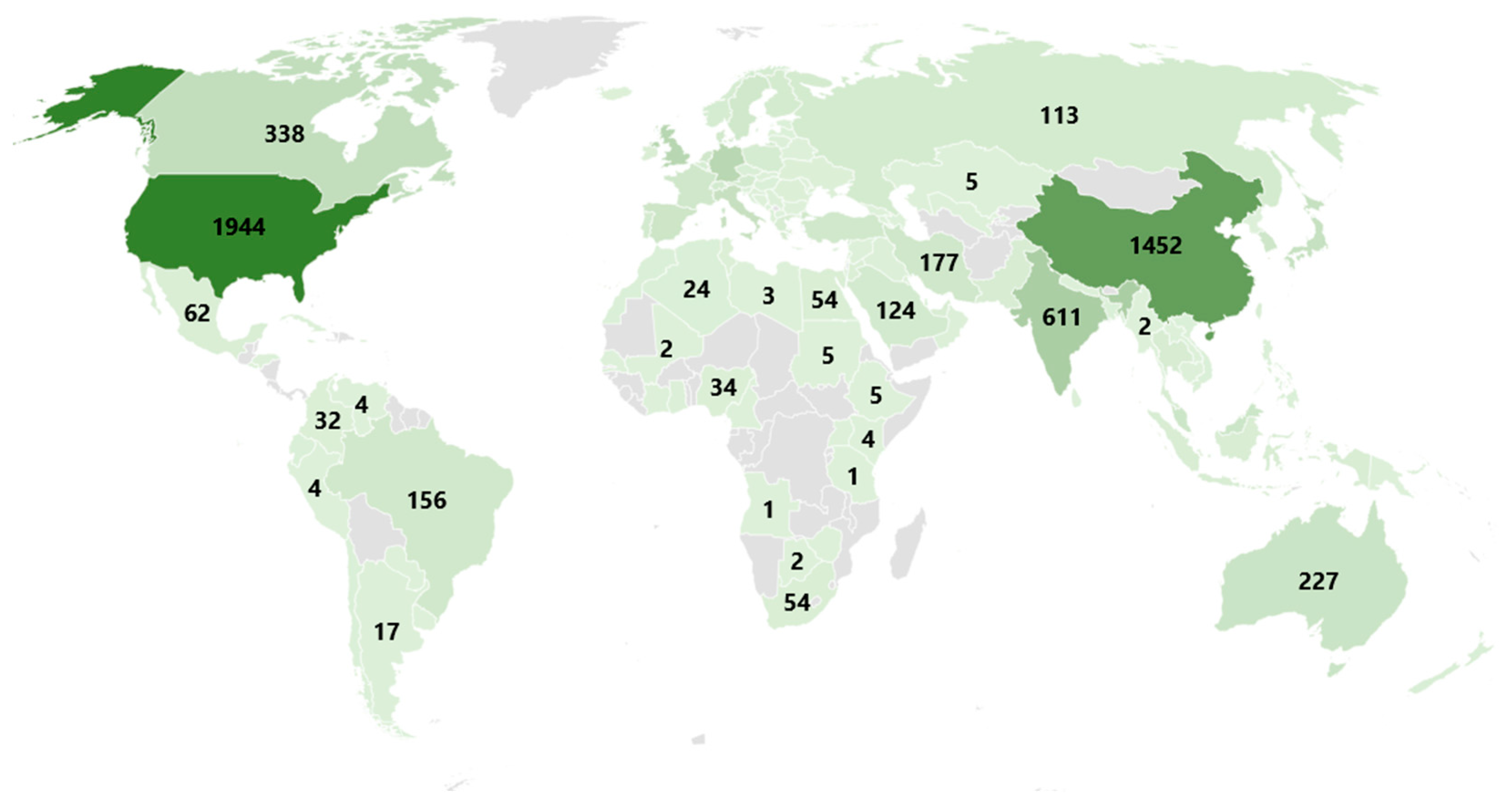
Figure 1. Worldwide publication trends obtained from Scopus with the keyword transportation energy demand.
Sustainability 14 16064 g001
Figure 2. Worldwide publication trends obtained from Scopus with the keywords transportation energy demand and greenhouse gas emissions.
Sustainability 14 16064 g002
Figure 3. The trends of input and output data along with road sector fuel consumption for the period between 1976 and 2017 (Adapted from [41]).
Sustainability 14 16064 g003
Figure 4. A simplified illustration of an ANN.
Sustainability 14 16064 g004
Figure 5. Conceptual illustration of the proposed AI-model for Saudi Arabia’s energy demand forecasting in the road transportation sector.
Sustainability 14 16064 g005
Figure 6. Comparative illustrations of the ANN and SVR models in terms of MSE index.
Sustainability 14 16064 g006
Figure 7. Energy consumption from road transport and model output of the neural network.
Sustainability 14 16064 g007
Figure 8. Road transport energy consumption and model output of the SVR.
Sustainability 14 16064 g008
Figure 9. Comparative illustrations of the actual versus machine learning model predicted energy demand of the road transportation sector of Saudi Arabia.
Sustainability 14 16064 g009
Figure 10. Comparisons of the performance measures (CC and IA) in predicting future transportation energy demand for the developed machine learning models.
Sustainability 14 16064 g010
Figure 11. Observed energy consumption and outputs of the neural network and the SVR models.
Sustainability 14 16064 g011aSustainability 14 16064 g011b
Table 1. The unit root test result.
At LevelADF (Lag Length)PP (Lag Length)
InterceptIntercept and TrendInterceptIntercept and Trend
E2.03 (1)−2.23 (0)2.42 (3)−2.54 (6)
GDP−0.50 (0)−1.92 (0)−0.50 (0)−2.06 (1)
P−1.18 (0)−1.04 (0)−1.43 (1)−1.31 (1)
U4.14 (3)−3.66 ** (4)4.65 (2)−3.95 ** (2)
V1.36 (1)−0.68 * (1)7.09 (2)−1.18 (2)
At first differenceInterceptIntercept and TrendInterceptIntercept and Trend
E−4.81 (0) *** −6.19 (0) ***−4.82 (2) *** −6.20 (1) ***
GDP−3.82 (2) ***−3.75 (0) **−3.84 (2) ***−3.73 (2) **
P−3.43 (0) **−3.39 (0) *−3.43 (0) **−3.39 (0) *
U−2.50 * (4)2.34 (3)−2.07 * (2)0.30 (2)
V−039 (0) *−2.00 (0)−0.39 (0)−2.00 (0)
Note: E, GDP, P, U, and V are road transport energy consumption, annual GDP, fuel price, urban population, and passenger vehicle number, respectively. The numbers in parentheses are lag lengths, while the asterisks (***, **, *) denote statistical significance at the 0.01, 0.05, and 0.1 levels, respectively.
Table 2. Results of the Johansen cointegration test.
Hypothesized Number of
Co-Integrating Equation(s)
r = 0r = 1r = 2r = 3r = 4
Trace statistics113.91 ***61.58 ***27.047.210.57
Maximum Eigenvalue statistics52.33 ***34.54 ***19.836.640.57
Note: *** indicate significance at 0.01 level.
Table 3. Summarized form of the co-integrating equation.
Dependent Variable: TE
Explanatory VariablesCoefficientsStandard Errort-Statistics
Constant11.813.710.86
GDP0.0030.0170.176
P−127.1035.91−3.54
U−17.732.53−7.00
V14.351.8219.23
Table 4. Granger causality test result.
Short-Run Granger Causality—F StatisticsLong-Run Granger Causality—t-Statistics
Ln (E)Ln (GDP)Ln (P)Ln (U)Ln (V)Error Correction Term (ECT)
Ln (E)-3.93 * (0.07)0.04 (0.85)3.63 * (0.08)0.20 (0.66)−1.58 (0.14)
Ln (GDP)1.52 (0.24)-8.02 ** (0.02)5.21 ** (0.04)4.53 * (0.05)1.98 * (0.07)
Ln (P)3.11 (0.10)0.01 (0.92)-0.01 (0.91)0.03 (0.86)0.45 (0.66)
Ln (U)0.60 (0.45)0.29 (0.60)0.79 (0.39)-3.31 * (0.09)1.91 * (0.08)
Ln (V)0.003 (0.96)2.17 (0.17)0.19 (0.67)3.02 (0.10)-0.19 (0.85)
Note: p-values are shown in parentheses, and the symbols ** and * denote statistical significance at the 0.05 and 0.1 levels, respectively.
Table 5. Performance measures of developed ANN and SVR models.
HeadingRMSE (MTOE)MAE (MTOE)MAPECCIA
Training Datasets (ANN)0.70.434.340.99240.9989
Testing Datasets (ANN)3.915.397.530.89320.9899
Training Datasets (SVR)0.00.000.0011
Testing Datasets (SVR)0.90.731.910.99250.9996
Publisher’s Note: MDPI stays neutral with regard to jurisdictional claims in published maps and institutional affiliations.