From Theory to Practice: Can LEAP/FAO Biodiversity Assessment Guidelines Be a Useful Tool for Knowing the Environmental Status of Livestock Systems?

Abstract

Biodiversity loss is a global concern, and agriculture is one of the economic sectors responsible for this impact. The assessment of ecosystems under the influence of livestock production is essential for knowing their integrity and ability to provide ecosystem services. The aim of this investigation was to evaluate the application of LEAP/FAO guidelines for quantitative assessment of biodiversity in the livestock sector at the local scale (farm level) in a group of six study cases in Uruguay. A set of 20 indicators was used, including seven key thematic issues: habitat protection, habitat change, wildlife conservation, invasive species, pollution, aquatic biodiversity, off-farm feed, and landscape-scale conservation. The results show that the LEAP biodiversity assessment guidelines can be useful to characterize the state of ecosystems under pastoral use and some specific components of their biodiversity, as well as assess the interaction of the production system with the environment and plan management accordingly. This work also provides an analysis of the methodology used and recommendations to facilitate its application by the sector. The results from the application of the indicators show a great deal of wild biodiversity that uses grazing systems based on native grasslands as habitats and the acceptable integrity of these ecosystems. On average, farms have 83% of their native ecosystem, with a value of 3.5 for the Ecosystem Integrity Index. In terms of the richness of different groups, there was an average number of species of 112 herbaceous plants, 48 woody plants, 48 spiders, 150 birds, and 14 fish. The main goal of this work is to help in the wider application of the guidelines by facilitating decisions about methodology, necessary resources, and technical support. Moreover, another goal is to show the importance of native grasslands-based livestock systems for biodiversity conservation.

1. Introduction

Biodiversity is essential for ecosystem functioning and human well-being through service provision, but the rate of species richness decline exceeds a hundred times the estimated normal rate between previous mass extinctions [1]. One of the main drivers of species extinction is habitat loss caused by human conversion of natural ecosystems to other uses, mainly for producing commodities for consumption [2]. Land use for animal production influences the earth system in a variety of ways, including local-scale modification of the environment, affecting a wide spectrum of issues (i.e., biodiversity, soil health, nutrient cycling, and the hydrology cycle) [3]. However, livestock systems differ in their impact and significance on biodiversity. At one extreme, undisturbed habitats could be impacted by the conversion of primary forests into pastures or feed crops [4,5,6]. At the other extreme, in places with a long livestock history, many organisms have specifically adapted to habitats associated with the presence of domestic herbivores, and they now play important roles in maintaining permanent grassland habitats with high biodiversity levels, as in Europe [7,8,9,10], America [11,12], Africa [13,14], and Oceania [15,16]. Occasionally, livestock can play a similar ecological role to that of wildlife (i.e., bison in North American rangelands [17]) or play important roles in seed dispersion [18].

Between these two extreme situations, a large number of impacts can be described. Grazing can be a cause of erosion by trampling and changing the soil’s physical and chemical properties, such as bulk density, moisture content, pH, and nutrient content [19,20]. Overgrazing can also lead to biodiversity loss by degrading plant community composition, diversity, and productivity [21]. Nutrient excess caused by excretion or fertilization can alter the nutrient cycle, promoting habitat changes [22], causing significant diffuse pollution by nitrogen and phosphorus [23], and consequently eutrophication and acidification in both terrestrial and aquatic ecosystems [24]. Acidification modifies species composition and the structure of terrestrial ecosystems [25].

Biodiversity has an essential role not only for its intrinsic value but also for the key role it plays in supporting ecosystem services that benefit human societies and economies [26,27]. Anthropogenic environmental changes will continue to cause biodiversity loss in the coming decades, with higher rates of species extinction that could threaten the stability of the ecosystem services on which humans depend [28]. It is therefore important to assess the state of biodiversity in livestock systems in order to monitor their current integrity and ability to continue providing ecosystem services. However, biodiversity assessment has its difficulties due to its intrinsic complexity (site specificity with different composition, structure, and function), scale issues, and problems related to reducing biodiversity assessment to a single measure or conservation objective [2]. Many quantitative indicators and assessment methods have been developed to evaluate biodiversity, but it still presents considerable challenges. Reaching an international consensus for the evaluation of the effects of production systems is still a work in progress [27,29].

In this sense, the Food and Agriculture Organization (FAO) has promoted a multi-stakeholder initiative that is committed to improving the environmental performance of livestock supply chains (Livestock Environmental Assessment and Performance; LEAP). The partnership integrates governments, the private sector, non-governmental organizations (NGOs), and civil society organizations (CSOs), which all identify the need for comparative and standardized indicators to switch the focus of dialogue with stakeholders from methods to improved management measures. The LEAP develops comprehensive guidance and methodology for understanding the environmental performance of livestock supply chains in order to shape evidence-based policy measures and business strategies [30].

Most of the LEAP guidelines recommend the use of Life Cycle Assessment (LCA) as the main methodology for environmental assessment [31]. Although the use of LCA in biodiversity assessment is considered a necessary trend [32] and there has been some effort towards adapting the methodology [33], it is still difficult to apply this complete methodology for biodiversity analysis at the local level [2]. This is because biodiversity is site-specific, and LCA biodiversity impacts reports will always be expressed in relation to a functional unit (e.g., per kg of carcass or live weight), with no agreed metrics to standardize this assessment. 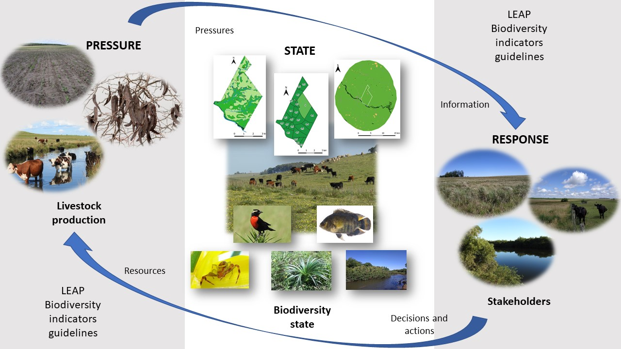For this reason, although the LEAP biodiversity guidelines for quantitative assessment [2] recommend several life cycle impact analysis (LCIA) models for regional to global assessment, they propose that the most suitable approach for local assessments is to use the Pressure-State-Response (PSR) indicators framework, which is based on causality. Indicators are used to assess the pressure of human activities (e.g., pollution, habitat, and climate change) that lead to changes in the state of the environment or the state of biodiversity (e.g., abundance, richness, or composition of species, ecosystem degradation). This assessment promotes responses (i.e., decisions and actions) from stakeholders (e.g., politicians and producers) aimed at achieving a more sustainable state, either by mitigating the negative effects by taking measures to reverse the damage or by conserving habitats and biodiversity [2].

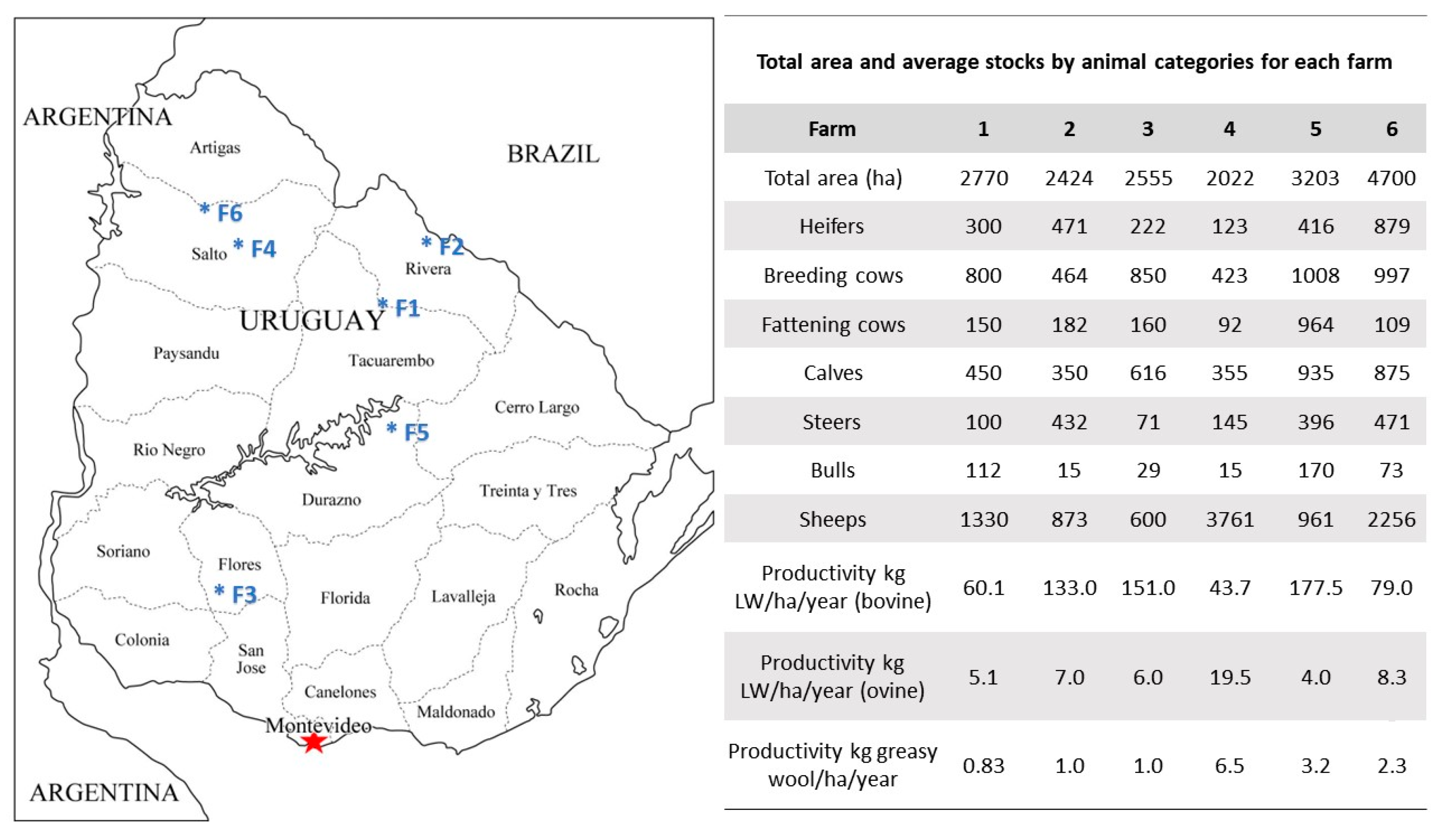
The objective of this investigation was to evaluate the application of the LEAP/FAO guidelines for quantitative assessment of biodiversity in the livestock sector [2] at the local scale (farm level) in a set of study cases in the livestock sector of Uruguay. The focus was on the feasibility of using all the recommended indicators, the selection of methodology, and the importance of interpreting the results based on the assessment’s scope and goal.

2. Materials and Methods

2.1. Study Cases

The investigation was carried out on six farms belonging to the Uruguayan Federation of CREA groups (FUCREA). The study cases were randomly selected from an anonymous database by some predetermined criteria: farms with a complete bovine cycle (breeding cattle to fattening steers) and sheep production; three of them with 100% of the native grasslands area; and the other three with a 25 to 30% substitution of native grasslands by cultivated pastures. The selection of study cases was carried out among full-cycle farmers so that all animal categories were present. A previous analysis of the databases made by CREA showed that systems with between 25 and 30% substitution of native grasslands by pastures represented a common model of pastoral systems, and 100% of native grasslands were common in traditional systems. Of the total number of cases in each category, the selected farms were drawn. These cases represent the reality of Uruguay, where mixed systems (cattle and sheep) are dominant, native grasslands are the base of pastoral systems, and the most common intensification initiative is the incorporation of cultivated pastures [34]. The farms are large-scale (2000 to 5000 hectares) and are located in different areas of the departments of Salto, Rivera, Durazno, and Flores. The localization of farms and productive characteristics are shown in Figure A1.

2.2. Set of Indicators

The LEAP guideline [2] provides a list of recommended biodiversity pressure-state-response indicators addressing seven key thematic issues: habitat protection, habitat change, wildlife conservation, invasive species, pollution, aquatic biodiversity, off-farm feed, and landscape-scale conservation. Each of these includes a number of quantitative and qualitative measures. In this investigation, the complete list was applied, and in some cases, a single indicator was composed of multiple variables or sources of information. It was because of the interest in evaluating more than one possibility for applying the indicator.

2.2.1. Habitat Protection Indicators

Three indicators were included: (a) the inventory of wildlife habitats under the farm’s influence, (b) the proportion of semi-natural habitats, and (c) grassland restoration initiatives.

To construct these indicators, maps of the living environments were made, which imply the spatial representation of the distribution of different communities in each farm, employing photo-interpretation of satellite images and field validation. The work was carried out using the free software Q-GIS (Version 3.16.12) [35] and based on orthophotos from 2018–2019 with a resolution of 0.32 m per pixel available for download in the Spatial Data Infrastructure of Uruguay [36]. Additionally, the geographic information layer was used in the raster format “grassland cartography” of Uruguay, where the country’s grasslands are classified, which is available on the website of the Agriculture Ministry [37]. Grassland restoration initiatives were identified through direct interviews with farmers.

2.2.2. Habitat Change

Four indicators were addressed: (a) soil erosion and soil erosion risk mapping and management plans implemented, (b) the proportion of the area with degraded soil, (c) the rate of habitat conversion, and (d) livestock density.

For the soil erosion and erosion risk indicator, a map developed by Carrasco and Beretta [38] was used. The authors estimated erosion in 99 drainage basins in Uruguay, analyzing and managing the information required by the universal equations of soil loss (USLE/RUSLE) to predict the amount of soil loss due to runoff in specific areas under certain management systems and crops [39]. The results were presented in a geographic information layer in which each polygon was assigned to a class. Each class identified by a color represents a range of soil loss in tons per hectare per year [38].

Information about the state of soil degradation was obtained by applying the Ecosystem Integrity Index (EII) [40], an environmental assessment tool whose main objective is to assess the agro-ecosystem’s state in relation to an “optimum” established for the ecoregion evaluated. This index has four dimensions, one of them is the state of the soil, valuating the vegetation cover, evidence of erosion, and predisposing conditions to degradation. A map was built for each farm that shows the value of the soil component of the EII for each paddock on a scale from 0 to 5. For paddocks with values equal to or less than 3.5, it was analyzed which of the characteristics evaluated were related to bad conditions.

The area or rate of habitat conversion was obtained from the environment map by calculating the proportion of native grasslands that were transformed into cultivated pastures, crops, forests, or dams. The density of cattle was related to the carrying capacity of the pastures in order to indicate if there was an excess of cattle. Stocking rate data were extracted from the farmer databases, which are periodically updated and closed annually. Livestock values were expressed in livestock units (LU), equivalent to an animal of 380 kg standard weight. For the carrying capacity of the native grasslands, the reference was the value of the “safe stocking rate” according to Saravia et al. [41], which establishes a reference for the number of heads of cattle per hectare considering the soil type. The calculation of the carrying capacity of the cultivated pastures was carried out based on bibliographic data on cultivated pastures’ yields and the cattle requirements [42,43].

2.2.3. Wildlife Conservation

Three indicators were included: (a) actions promoting high-value conservation species; (b) particular species with high conservation values; and (c) species richness or diversity. This last indicator can include a lot of different groups and measurable variables, which can turn it into a multidisciplinary assessment.

In the present investigation, the vegetal communities included were forests (woody species richness and diversity) and herbaceous communities in reference paddocks (richness, different strata cover rate, and community map). In the case of fauna, spiders, birds, and fish were included.

A reference paddock was selected for each farm to evaluate the grassland communities. A preliminary assessment of each paddock was carried out in late 2019, during which high-definition aerial images were generated using a drone and the main plant communities to be characterized in subsequent samplings were defined. The plant communities were recognized physiognomically based on the density and height of the vegetation and according to the geomorphological characteristics of the regions in which they develop, following Lezama et al. [44]. Vegetation surveys were carried out during the summer and spring of 2020 following the phytosociological method [45]. Three sampling points representative of the global variation present in the paddock were selected for each of the different plant communities identified. At each sampling point, a 5 × 5 m plot was implemented, in which all vascular plant species present were recorded and specimens of those species that required observation under a magnifying glass were collected to be identified later. A percentage of the aerial cover of each species was visually estimated following the Braun-Blanquet [46] abundance scale for values under 5% and in steps of 5% for higher values. The coverage of species in the lower stratum was estimated using a 50 × 50 cm quadrant, placed at three different points within each plot. Additionally, the height and number of strata were recorded, as well as the total coverage of each stratum. Each species was subsequently classified according to its origin (i.e., native or adventitious) [47] and life form [48].

In the case of woody communities in native forests, the protocol for integrity assessment of the REDD+ initiative was applied [49] on farms with more than 1% of the farm area occupied by native forest. It included at least two transects per farm of 100 m long and 2 m in width. In these transects, species, the number of individuals, and size categories were recorded, and the Shannon diversity index [50] was calculated. Along the transect, five points were selected for seedling counting and assessing the cover of herbaceous plants, mulch, and canopy cover using one-square-meter plots. In addition, to calculate richness, woody species were also recorded during the application of the Ecosystem Integrity Index [40].

Arthropods were collected with two complementary techniques, pitfall traps and aspirations [51]. Pitfall traps consisted of open-top plastic containers buried in the ground slightly below the surface, which were partially filled with a preservative solution (50% propylene glycol) to preserve the arthropods that fell inside [51]. One reference paddock with native grasslands was selected in each study case, and in those with cultivated pastures, one additional paddock with annual pastures was selected. Traps were installed in each paddock in a 100-m transect, placing a pair of traps every 10 m, separated from each other by two meters. The traps were installed every season for one year and remained active for seven days; after that time, they were removed and taken to the laboratory for later identification. Complementary aspirations of the herbaceous layer were carried out using a modified garden vacuum cleaner (g-vac). Ten sample units of 1 m² were taken close to each pair of traps following the transect. Each sampling unit corresponded to one minute of aspiration, and the samples were placed in bags with 70% alcohol duly labeled. The content of the traps and aspirations was processed, and the collected arthropods were separated for posterior identification. In this study, only spiders were taxonomically classified, and the rest of the arthropods were preserved for future analysis. Spiders were identified at the species/morphospecies level. Rarefaction curves were made based on the number of samples, in order to estimate the efficiency of samplings. In addition, a non-parametric estimator of species richness (Chao 1) and the Shannon diversity index [50] were calculated. These analyses were made with the software EstimateS 9.1 [52]. The efficiency of both techniques was compared using the data of the paddock (Farm 3, native grassland) with more spiders and species. Abundance and species richness of spiders collected with g-vac and pitfalls were compared using t-tests. The data were log-transformed because they did not approach a normal distribution. These analyses were performed with the software INFOSTAT (ver.2016) [53].

For bird sampling, as recommended by Gibbons and Gregory [54], Mackinnon’s lists were used. They consist of visual and/or auditory records along paths (not previously defined) where the observed species are recorded until reaching a certain amount (15 in this case), then a new list is started where the already observed species can be included again [55]. This methodology was applied in the predominant environments of each establishment (native grassland, cultivated pasture, and forest). The bird samples were carried out in three seasons (spring, summer, and winter).

Species with high conservation values were identified for woody and herbaceous plants, birds, fish (see pollution and aquatic biodiversity indicators), and spiders based on the official Uruguayan lists of priority species for conservation [56,57]. Actions implemented to promote these species were identified through direct interviews with farmers.

2.2.4. Invasive Species

Two indicators were included: (a) a management plan in place for the control of invasive species and (b) the presence and abundance of invasive alien species.

The invasive flora species present in the farms were recorded during the application of the Ecosystem Integrity Index and with the lists of herbaceous and woody species from the richness studies. Invasive fauna species were identified from the bird and fish lists. The publications of Soutullo et al. [56], Brazeiro et al. [58], and Proyecto REDD+ Uruguay [59] were used as references.

Information about the existence of management plans for the control of invasive alien species resulted from interviews with the farmers and the observation of the management system and the applied practices.

2.2.5. Pollution and Aquatic Biodiversity

Four indicators were used: (a) management plan in place for the application of ecotoxic agrochemicals; (b) nutrient management plan in place to rationalize fertilizer application; (c) length/proportion of protected waterways; and (d) ecological indicators of eutrophication or water quality.

Information on nutrient and agrochemical (herbicides, pesticides, veterinary products, and fertilizers) management, including application following manufacturers’ guidelines, safe storage, measures to avoid application in sensitive habitats, and actions to minimize the risk of nutrient loss, resulted from interviews with the farmers and the observation of the management system and the applied practices.

Streams can be protected through livestock exclusion (e.g., fencing), edges, or buffer strips. In the “riparian zones” component of the Ecosystem Integrity Index [40], the width of the buffer zone of all the water courses of each farm was recorded. The presence of fences was identified through satellite images and field surveys.

Fish were collected using electric fishing on two streams per farm in winter and summer. Following the methodology proposed by Teixeira de Mello et al. [60], 50 pulses were performed in a 50-m section of each stream. Once the fish were collected, they were euthanized with an overdose of 2-phenoxy-ethanol (5 ml·L⁻¹), a technique approved by the Honorary Commission for Animal Experimentation (CHEA). The collected individuals were fixed in 10% formaldehyde and transported to the laboratory for further analysis. All individuals was classified at the species level. The number of individuals captured were corrected following Texeira de Mello et al. [60], estimating density (ind/m²) and fish biomass per square meter (BM, g/m²). To avoid species abundance effects, rarefaction curves were generated with the statistical package iNEXT to calculate the observed and estimated richness, thus making possible the evaluation of this sampling method’s performance [61,62]. Finally, species richness, number of individuals, density, and biomass per square meter were compared between seasons using a repeated measures ANOVA in the free R software (version 4.1.3) [63].

At each site, physicochemical parameters of the water were measured using a YSI 600OMS-V2 multiparametric probe (pH, conductivity, temperature, and dissolved oxygen), Xylem Inc., Washington DC, USA. Additionally, water samples were taken for subsequent nutrient analysis in the laboratory (total phosphorus and total nitrogen). All physicochemical variables were compared between seasons using a repeated measures ANOVA in the R software (version 4.1.3) [63].

2.2.6. Off-Farm Feed

Three indicators were included in this section: (a) an inventory of the off-farm feed being used established; (b) traceability systems for feed stuff implemented; and (c) the share of imported feed–total from areas that are certified/deforested/of high conservation value.

Information about the composition and volume (weight) of the off-farm feed and its production origin was obtained from interviews with farmers and searches for information.

2.2.7. Landscape-Scale Conservation

Two indicators were addressed: (a) measures to promote connectivity identified and implemented, and (b) landscape heterogeneity.

Information about the heterogeneity of the landscape was obtained from the land use and land cover annual map 2019 of MapBiomas Pampa, Collection 1 [64]. Using the free software Q-GIS (version 3.16.12) [35], the map was cut with a buffer area of 10 km around each farm and processed using the Landscape Ecology Statistics (LecoS) plugin [65] to obtain the landscape proportion, largest patch index, and effective mesh size [66,67] of each land use or cover (Forest Formation, Forestry, Wetland, Grassland, Farming, Non-Vegetated Area). In addition, through the interpretation of the environment maps, the physical elements that impede the mobility of organisms along natural corridors or habitats and the measures implemented to overcome them were identified.

3. Results

3.1. Habitat Protection Indicators

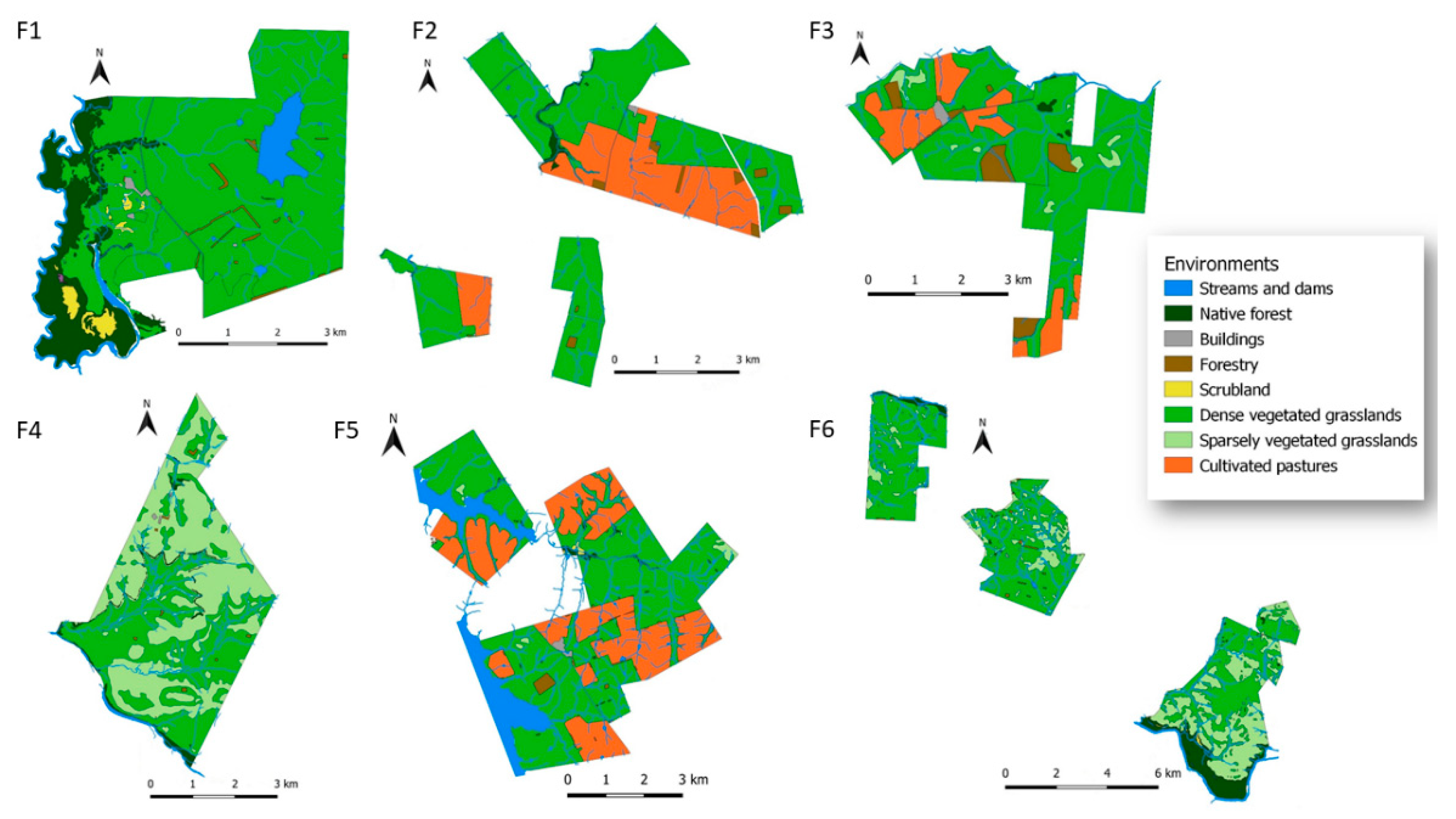
A geographic information system (GIS) was used to map the different natural and modified environments of farms (Figure A2).

None of the properties are included in the National System of Protected Areas of Uruguay (SNAP). The only protected environment with legal regulations is the native forest [68]. None of the farms had degraded areas under restoration management.

Table 1. Proportion of different environments in the studied farms (F).

Environment	F1	F2	F3	F4	F5	F6
Dense vegetated grassland	76.5	66.5	66.1	46.4	63.8	65.2
Sparsely vegetated grassland	0.0	0.0	2.2	50.5	0.9	26.2
Cultivated pastures	0.0	29.1	25.1	0.0	32.1	0.0
Native forest	15.4	1.5	0.6	2.7	1.0	7. 7
Scrubland	1. 9	0.0	0.0	0.0	0.2	0.1
Dams	4.5	0. 6	0.3	0.0	0.6	0.3
Buildings	0.6	0.4	0.7	0.1	0.4	0.1
Forestry	1.1	2.0	5.1	0.3	1.1	0.4
Total modified	6.2	32.0	31.2	0.5	34.2	0.8
Total natural	93.8	68.0	68.8	99.5	65.8	99.2

shows the percentage of semi-natural (densely vegetated grasslands, sparsely vegetated grasslands, and native forests) and modified environments (cultivated pastures, forestry, dams, and buildings) for each farm. The dominant vegetation on all farms was grassland.

3.2. Habitat Change

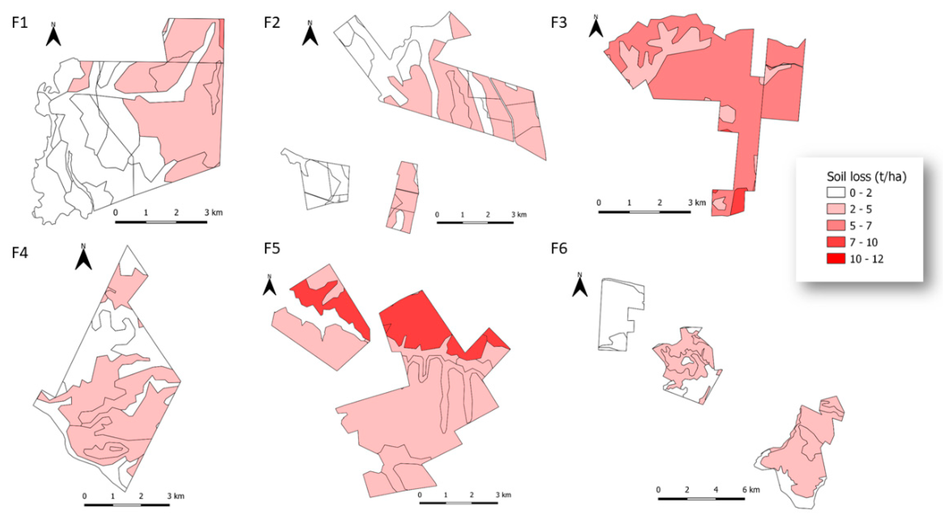
Based on the study of Carrasco and Beretta [38], part of the soils of farms 3 (2%) and 5 (24%) (F3 and F5, Figure A3) would experience an average annual soil loss of 7 ton/ha/year.

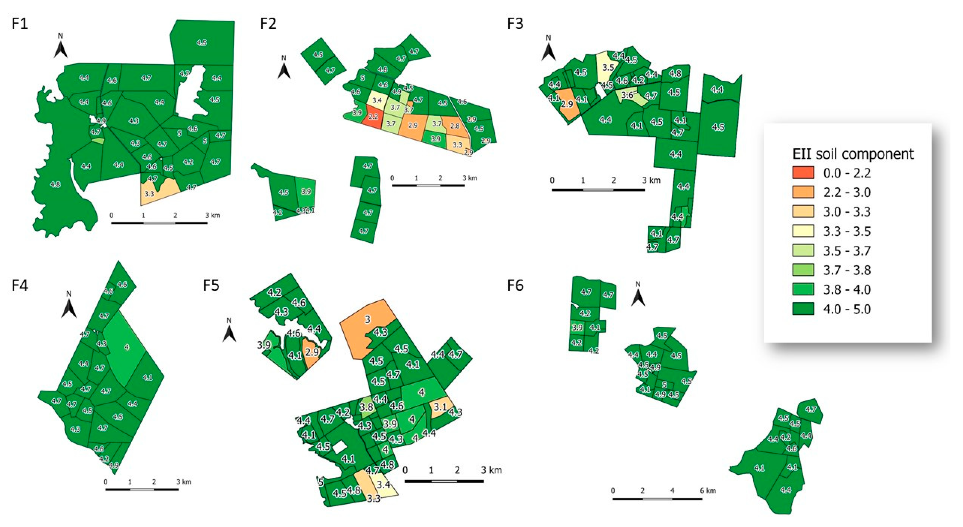
In farms 1, 2, 3, and 5, the proportion of area with values of the soil component of the EII lower than 3.5 was 2, 11, 6, and 15%, respectively. In farms 2, 3, and 5, the lowest values for the soil component generally coincided with cultivated pastures. The main reason for the EII soil component rating drop in these paddocks is the proportion of bare ground recorded. In farms 4 and 6, there were no values lower than 3.5 (Figure A4).

All farms with cultivated pastures (F2, F3, and F5, Figure A2) have a management plan to prevent soil erosion. In all farms, direct sowing is used, perpendicular to the slope. The buffer zones around the water courses or drains are not sown.

According to the livestock holding capacity calculated for cultivated pastures and the concept of “safe stocking rate” for native grassland [41], which establishes references for each ecoregion of the country, farms 1, 4, and 6 were over the sustainable carrying capacity of the farmlands (

Table A1. Livestock stocking used and carrying capacity for each farm. B: bovines, S: sheep, LU: livestock units, NG: native grassland, CPCC: cultivated pasture carrying capacity, TCC: total carrying capacity.

Farm	B	S	Others	Total LU/ha	“Safe Stocking Rate” NG	CPCC	TCC
1	0.70	0.08	0.14	0.92	0.85–0.90	0.00	0.85–0.90
2	0.78	0.06	0.06	0.90	0.80–0.85	1.09	0.91
3	0.70	0.04	0.03	0.77	0.70–0.75	1.21	0.86
4	0.41	0.31	0.02	0.74	0.65–0.70	0.00	0.65–0.70
5	0.81	0.04	-	0.85	0.85–0.90	1.17	0.99
6	0.61	0.08	0.02	0.71	0.65–0.70	0.00	0.65–0.70

).

The habitat conversion area, for farms 1, 4, and 6, in which the forage base of the productive system is based exclusively on native grasslands, had a substitution area of only 6.2, 0.5, and 0.8%, respectively. Farms 2, 3, and 5, in which there was a percentage of substitution of native grasslands for cultivated pastures, presented a modified area of 32, 31, and 34%, respectively. Table 1 shows the proportion of habitat conversion for each farm.

3.3. Wildlife Conservation

3.3.1. Flora

No special management or actions were implemented by farmers for the conservation of tall grasslands, which is an endangered ecosystem and is the habitat with the highest number of threatened species.

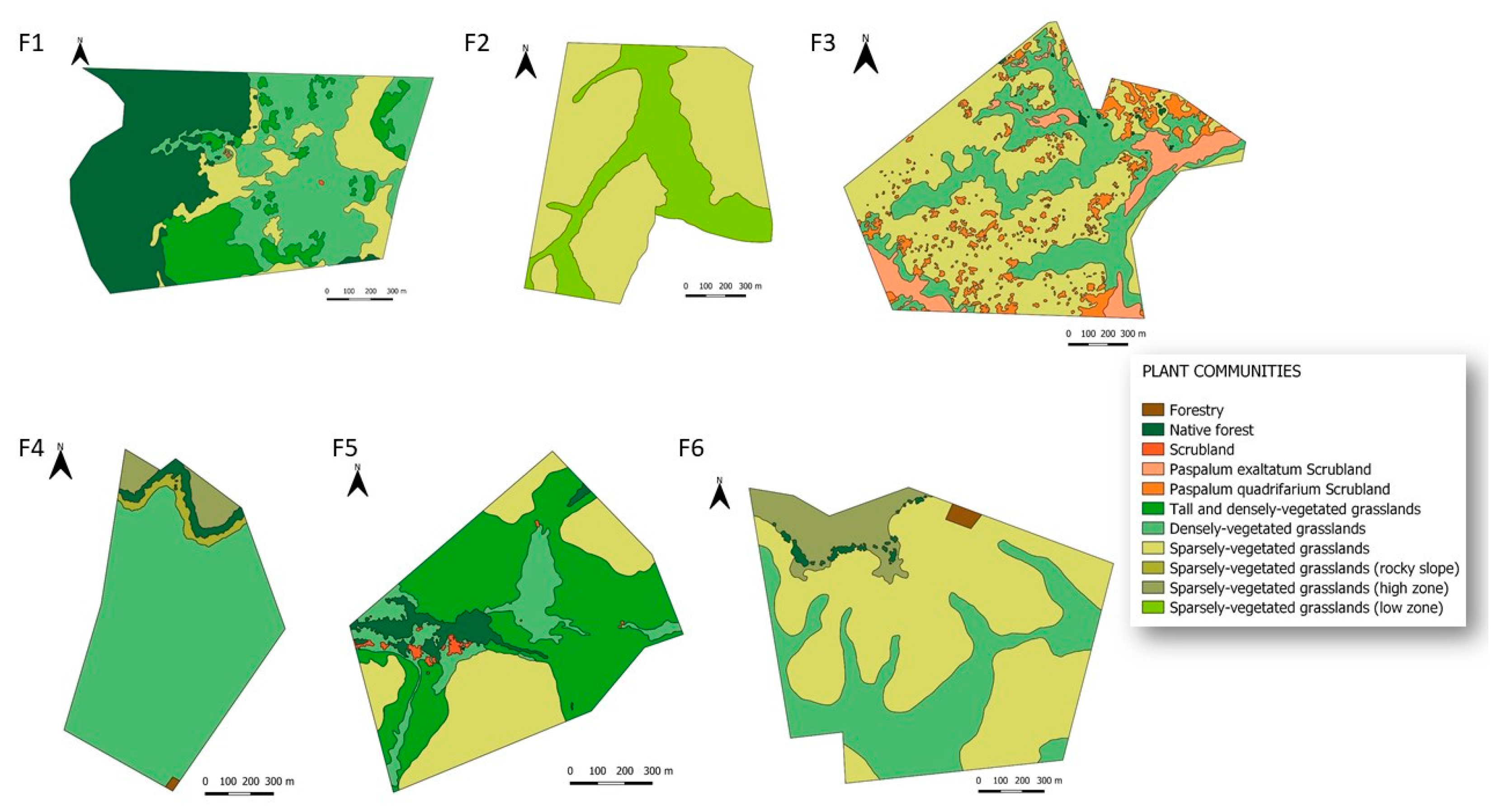
Abundant information was obtained for the selected groups of flora and fauna. For the herbaceous vegetation of native grasslands, between two and four different communities were recognized on each farm (Figure A5). These communities include sparsely vegetated grasslands, densely vegetated grasslands, tall and densely vegetated grasslands, and scrubland.

Results of the phytosociological surveys of these communities found a total of 104, 54, 138, 149, 119, and 114 species of vascular plants on farms 1 to 6, respectively. The families with the highest species richness were Poaceae, Asteraceae, and Cyperaceae for farms 1, 2, 3, and 5, while they were Poaceae, Asteraceae, and Fabaceae for farms 4 and 6 (

Table 2. Richness of herbaceous vegetation.

Farm	Nº of Families	Nº of Species	Most Species-Rich Families (Nº spp.)
1	23	103	Poaceae (32) Asteraceae (25) Cyperaceae (11)
2	13	53	Poaceae (29) Asteraceae (6) Cyperaceae (4)
3	33	136	Poaceae (41) Asteraceae (26) Cyperaceae (14)
4	42	149	Poaceae (36) Asteraceae (23) Fabaceae (9)
5	25	118	Poaceae (30) Asteraceae (24) Cyperaceae (12)
6	31	114	Poaceae (32) Asteraceae (17) Fabaceae (8)

).

For Poaceae, the dominant species were Axonopus fissifolius (Raddi) Kuhlm (farms 1 and 2), Paspalum notatum Flüggé (farms 4, 5, and 6), and Andropogon lateralis Nees (farm 3). For Asteraceae, Baccharis coridifolia DC. (farms 2, 4, 5, and 6), Vernonanthura nudiflora (Less.) H. Rob. (farm 1), and Baccharis trimera (Less.) DC (farm 3). For Cyperaceae, Cyperus brevifolius (Rottb.) Endl. ex Hassk (farm 1), Eleocharis dunensis Kük (farm 2), Carex bonariensis Desf. Ex Poir. (farm 5), Cyperus polystachyos Rottb. (farm 3), Carex phalaroides Kunth (farm 4), and Eleocharis montevidensis Kunth (farm 6). For Fabaceae, Galactia marginalis Benth (farms 2 and 5), Adesmia punctata var. sessiliflora Davyt and Izag. (farm 3), Adesmia bicolor (Poir.) DC. (farm 4), Trifolium polymorphum Poir (farm 6), and Adesmia sp. (farm 1).

A total of 13 herbaceous species considered a priority for conservation in Uruguay were recorded across five of the farms, with farm 2 being the only one where no such species were found (

Table 3. Priority herbaceous species for conservation recorded by farm (F).

Family	Species	F1	F2	F3	F4	F5	F6
Euphorbiaceae	Acalypha senilis Baill.				X
Apiaceae	Ammoselinum rosengurttii Mathias & Constance				X
Orchidaceae	Bipinnula biplumata (L. f.) Rchb. f.			X
Cyperaceae	Carex uruguensis Boeckeler					X
Poaceae	Danthonia rhizomata Swallen			X
Poaceae	Digitaria cuyabensis (Trin.) Parodi					X
Poaceae	Digitaria eriostachya Mez	X
Asteraceae	Hypochaeris rosengurttii Cabrera			X
Asteraceae	Lessingianthus glabratus (Less.) H. Rob.	X
Solanaceae	Nierembergia calycina Hook.				X
Solanaceae	Solanum commersonii Dunal	X
Euphorbiaceae	Tragia incana Klotzsch ex Müll. Arg.					X
Asteraceae	Trichocline incana (Lam.) Cass.			X

).

Overall, 18 exotic herbaceous species were found throughout the surveyed paddocks of all farms, but most of them with average spatial coverage values below 1% in any given community. The only exception was Cynodon dactylon (L.) Pers., which was found to be very prevalent in farms 1 and 5, but mostly in farm 2, with coverage values ranging up to nearly 75% in some plots and averaging 42% for one of the communities. Incidentally, farm 2 had the lowest amount of plant families and species out of the six farms by a considerable margin. The complete lists of species and their relative coverage within each community are presented in Tables S1–S7.

In the case of woody native forest communities, 63, 41, 27, 55, 36, and 64 species of native trees were listed for farms 1 to 6, respectively (Table S8). Through the REDD+ integrity assessment protocol, the richness, Shannon diversity index, and soil and canopy cover (

Table 4. Analysis of tree richness, diversity, and soil and canopy cover of native forests.

Farm	Richness	Shannon Index	Average Number of Seedlings (Plants/m2)	Soil Cover %			Canopy Cover
				Herbaceous Plants	Shrubs and Tree Seedling	Mulch
F1	23	2.15	30.3	8.9	12.0	88.4	83.6
F2	20	2.41	4.3	13.7	0.8	20.9	82.8
F4.1	28	2.84	12.3	32.5	17.6	50.7	81.2
F4.2	19	2.54	6.7	12.8	1.1	58.3	80.3
F6	33	2.91	7.2	24.1	6.0	62.2	80.5

) were obtained for four farms that had more than 1% of their area occupied by native forest. Farm 4 had two types of native forests, riparian (F4.1) and ravine (F4.2), which were sampled separately.

Three woody species considered a priority for conservation in Uruguay were recorded: Allophylus guaraniticus Radlk. on farm 4, Banara umbraticola Arechav. on farm 4 and 6 and Pomaria rubicunda (Vogel) B.B. Simpson and G.P. Lewis on farm 6.

3.3.2. Fauna

In the spiders’ study, 13,406 individuals belonging to 28 families were collected, among which the families Linyphiidae (17.5%), Philodromidae (13.7%), Lycosidae (13.2%), Salticidae (9.7%), Oxyopidae (8.2%), Araneidae (7.4%), Anyphaenidae (6.7%), Theridiidae (6.1%), Thomisidae (4.1%), and Hahniidae (3.8%) were the 10 most abundant of the entire sample, representing 90.6% of the total. One hundred and three species/morphospecies were identified out of a total of 3268 adults (Table S9).

Table 5. Number of species and diversity (Shannon) of spiders present on each farm. F: farm; NG: native grasslands; P: cultivated pastures.

	F1	F2	F2	F3	F3	F4	F5	F5	F6
	NG	NG	P	NG	P	NG	NG	P	NG
Species richness	50	47	36	59	33	46	52	31	36
Shannon diversity index	3.21	3.05	2.72	3.31	3.06	3.06	3.41	2.94	3.02

shows the values of species richness and diversity (Shannon’s index) of the studied paddocks. The sampling efficiency was similar in all the sampled paddocks, and it was observed that all the species’ rarefaction curves approximated the asymptote (Figure 1).

Significant differences were found in the number of spiders and the number of species between collection techniques (t = 6.45, p < 0.0001; t = 6.49, p < 0.0001, respectively;

Table 6. Comparison of the collection efficiency of two collection techniques used in the natural grassland of Farm 3.

	G-VAC	PIT-FALLS	BOTH
Number of spiders	2259	245	2504
Number of adult spiders	393	140	533
Number of species	42	34	59
Number of estimated species (Chao 1)	51.97	51.97	79.02
Shannon diversity index	3	2.81	3.31

). Regarding the differences between the species recorded by technique, more exclusive species were reported with g-vac than with pitfalls (Figure 2). In total, 59 species were recorded with both techniques. More individuals and species of spiders were collected in the warm seasons, registering almost the same number of species in spring and summer, although more individuals were recorded in summer and 20 species were found exclusively in this season (

Table 7. Number of individuals and species of spiders collected per season using pitfalls and G-vac techniques.

	Season
	Autumn	Winter	Spring	Summer
Number of spiders	2350	3386	3323	4347
Number of species	43	53	67	68
Number of exclusive species	5	4	6	20

).

Two species of spiders considered a priority for their conservation in Uruguay were registered: Mesabolivar tandilicus (Pholcidae) on farm 1 (only in native grassland) and Aglaoctenus lagotis (Lycosidae) on farms 1 and 2.

The number of bird species recorded was 170, 148, 127, 132, 175, and 145 from farms 1 to 6, respectively (Table S10). Of these species, 31 are considered a priority for their conservation in Uruguay.

Table 8. Priority bird species for conservation recorded by farm (F).

Species	F1	F2	F3	F4	F5	F6
Anthusnattereri (Ochre-breasted Pipit)				X
Aramusguarauna (Limpkin)	X	X		X	X	X
Bartramialongicauda (Upland Sandpiper)		X	X	X	X	X
Cairinamoschata (Muscovy duck)	X				X
Calidrisfuscicollis (White-rumped Sandpiper)		X
Cariamacristata (Red-leggedSeriema)	X	X		X	X	X
Circus cinereus (Cinereous Harrier)	X	X			X
Cistothorusplatensis (Grass Wren)	X				X
Coragypsatratus (Black Vulture)				X
Coscorobacoscoroba (Coscoroba Swan)	X	X			X
Cranioleucasulphurifera (Sulphur-throated Spinetail)					X
Cyanocompsabrissonii (Ultramarine Grosbeak)						X
Cygnus melancoryphus (Black-necked Swan)	X				X
Donacospizaalbifrons (Long-tailed Reed-Finch)	X		X		X
Emberizoidesherbicola (Wedge-tailed Grass Finch)	X
Falco peregrinus (Peregrine Falcon)			X
Geranoaetusmelanoleucus (Black-chested Buzzard-eagle)			X			X
Gnorimopsarchopi (Chopi Blackbird)	X	X	X	X	X	X
Limnoctitesrectirostris (Straight-billed Reedhaunter)	X
Nothura maculosa (Spotted Nothura)	X	X	X	X	X	X
Oreopholusruficollis (Tawny-throated Dotterel)			X			X
Paroariacoronata (Red-crested cardinal)	X	X	X	X	X	X
Pluvialisdominica (American-Golden Plover)		X
Porzanaflaviventer (Yellow-breasted Crake)						X
Rhea americana (Greater Rhea)	X	X	X	X	X	X
Spartonoicamaluroides (Bay-capped Wren-spinetail)					X
Sporophilacinnamomea (Chestnut Seedeater)			X		X
Sporophilaruficollis (Dark-throated Seedeater)			X
Tryngitessubruficollis (Buff-breasted Sandpiper)				X
Turdusleucomelas (Pale-breasted Thrush)	X			X
Xolmisdominicanus (Black and White Monjita)			X		X

shows a list of them and their presence by farm.

3.4. Invasive Species

Few invasive alien species were detected from several taxonomic groups. The presence of herbaceous invaders such as Cynodon dactylon was recorded in all the farms, Senecio madagascariensis Poir. in farms 1, 3, and 5, and Eragrostis plana Nees. in farms 1 and 2.

Within the woody species, individuals of Gleditsia triacanthos L. were found on farms 1, 2, 3, and 4, Populus alba L. on farm 1, Melia azedarach L. on farm 6, and individuals of Pinus spp. on farm 1. Of these species, only G. triacanthos was considered to have a high level of presence, corresponding to farm 1.

Sturnus vulgaris, an invasive bird species, was recorded in farms 3, 4, 5, and 6, and Carduelis carduelis on farm 3.

Invasive fish species were not detected in any of the analyzed streams.

Farms 1 and 2 had a management plan for the control of E. plana that consisted of the application of glyphosate with a backpack, locally on the detected plants. Farm 2 also controlled G. triacanthos by cutting its trees, and farm 5 controlled S. madagascariensis by managing the sheep stock.

3.5. Pollution and Aquatic Biodiversity

All farms apply phosphorus (P) fertilizers, and those with cultivated pastures also use nitrogen (N). In all farms except F1, soil analysis is carried out before fertilization, and a certain distance is kept from water courses to reduce the risk of nutrient loss through leaching and run-off.

Herbicides were used by all farms, except F4, and all used veterinary products. All farmers stated that the applications are carried out according to factory or technical recommendations and away from water courses. Plastic waste and packaging of agrochemicals and fertilizers are safely stored on all farms to be later transferred to plastic recycling plants, except for those on farm 5 (F5), which are taken to garbage dumps or burned on the farm because there are no recycling centers in the area.

Fencing for livestock exclusion was only identified in some streams on farms 3 and 5. A stream was recorded on farms 2, 3, and 5 with a thin buffer zone (between 1 and 5 m wide). The other streams in all the properties had a buffer zone width greater than 15 m.

3.5.1. Water Quality

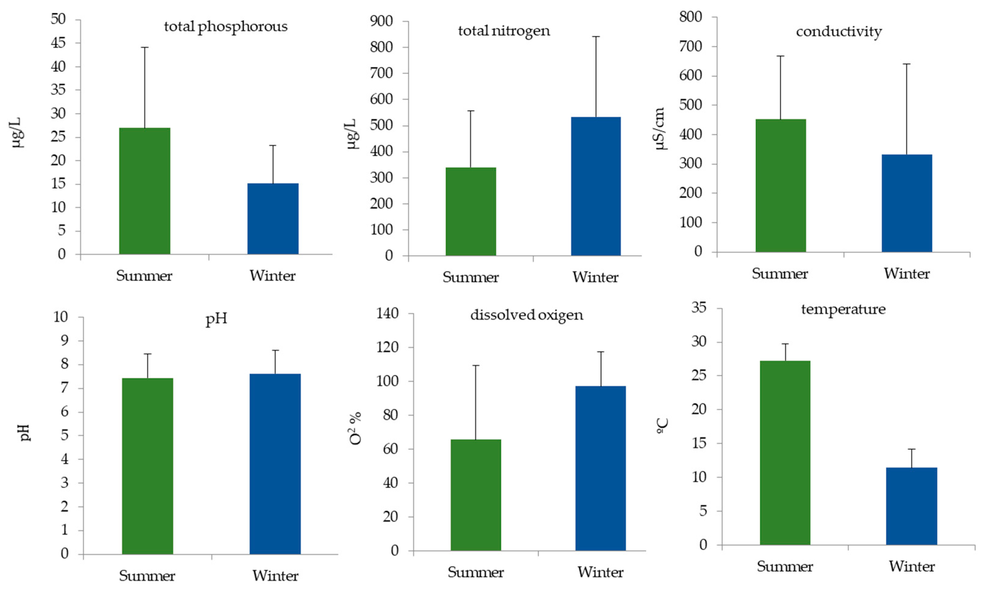
Stream water quality parameters showed variability between farms and with season (between summer and winter). Water temperature was significantly higher in summer than in winter (F = 1160, p < 0.00001), while the concentration of dissolved oxygen in water as well as the percentage of oxygen saturation were higher in winter than in summer (F = 6.27, p = 0.04 and F = 25.01, p = 0.001, respectively). Water conductivity was significantly higher in summer (F = 6.59, p = 0.03), while specific conductivity (corrected at 25 °C) did not show differences between both seasons. Since conductivity is temperature-dependent, differences between summer and winter are the result of water temperature and are not related to other environmental factors.

Total nutrients in water showed lower p values with means of 27 µg/L in summer and 15 µg/L in winter, and intermediate to high N values with means of 341 µg/L for summer and 533 µg/L in winter. Another important parameter that showed high variability was dissolved oxygen, with lower values in the summer (Figure 3). It is important to highlight the low water quality of some streams. In summer, systems F4.2 and F5.1 presented the highest values of total nitrogen (both with 706 µg/L) and anoxia values of 1.24 mg/L (16.7% O₂ saturation) and 0.62 mg/L (8.4% O₂ saturation). Moreover, sites F2.1 and F3.1 presented hypoxia with 2.58 (31.0% O₂ saturation) and 3.12 mg/L (36.4% O₂ saturation), respectively. Contrarily, site F6.2 presented oxygen supersaturation of 125.9% (9.36 mg/L). In winter, the maximum values of total nitrogen were detected in F3.1 and F4.2, with 1384 and 743 µg/L respectively. At this time, the sites F4.2 and F5.1 presented oxygen supersaturation values of 117.7% and 134.8%, respectively.

3.5.2. Fish Community

A total of 10,951 individual fish belonging to 13 families and 46 species were collected in the summer and winter. The families with the highest species richness were Characidae (34.8%), Cichlidae (21.7%), Loricariidae (8.7%), and Heptapteriidae (6.5%). Considering the number of individuals, the family with the highest abundance was Poecilidae (71.7%), followed by Characidae (18.1%), and Cichlidae (4.9%) (Table S11). The great abundance of the Poeciliidae family corresponds to individuals of Cnesterodon decemmaculatus (7024 individuals) collected at site F3.1, which is the stream with the lowest species richness, with only six species combined in both summer (6) and winter (4).

Richness, number of individuals, density, and biomass were higher in summer than in winter (

Table 9. Fish community descriptors for summer and winter.

Variable	Summer	Winter	F	p-Value
	Median ± SD	Median ± SD
Richness	14.1 ± 5.5	5.5 ± 4.2	0.0131	0.91
N individuals	1295.8 ± 2990.8	814.7 ± 1397.1	0.8467	0.38
Density (ind/m2)	13.9 ± 37.9	9.0 ± 14.7	0.4013	0.54
Biomass (g/m2)	3.9 ± 2.8	2.8 ± 11.9	0.6069	0.45

). The difference in species richness between both seasons corresponds to a higher richness per stream but strictly does not represent a higher number of total species collected in the summer (43 species) than in the winter (41 species). The species exclusively collected in summer were: Ancistrus taunayi, Gymnogeophagus peliochelynion, Hisonotus charrua, Oligosarcuso ligolepsi and Synbranchus marmoratus; during winter, there were: Characidium tenue, Hyphessobrycon togoi, and Rhamdella longiuscula.

The estimated species richness (via rarefaction) at the stream level was higher or equal in eight of the eleven streams, following the general pattern observed. However, F1.2, F4.1, and F6.2 showed an unexpected pattern with higher species richness in winter. Moreover, Shannon’s diversity follows a pattern similar to that of richness (

Table 10. Observed and estimated richness and Shannon diversity index for each stream in summer and winter.

Season	Index	Farm	F1		F2	F3		F4		F5		F6
		Stream	1	2	1	1	2	1	2	1	2	1	2
Winter	Richness	Observed	15	15	19	4	14	16	20	11	13	15	15
		Estimated	19	31	20	4	22	17	20	13	13	21	18
	Shannon	%	77	49	94	100	64	95	98	83	99	71	85
		Observed	7.11	8.77	10.38	1.15	4.75	10.87	5.23	6.89	3.55	10.90	9.55
		Estimated	7.51	11.54	11.50	1.15	5.04	12.49	5.30	7.90	3.62	13.32	10.72
Summer	Richness	Observed	18	5	19	6	21	10	17	14	19	16	10
		Estimated	20	5	25	6	22	12	21	16	23	22	13
	Shannon	%	90	91	75	100	93	82	81	86	83	73	77
		Observed	8.00	4.05	9.85	1.15	11.97	5.42	8.32	9.39	4.39	11.21	6.60
		Estimated	8.26	4.51	10.97	1.15	12.60	5.89	8.98	10.07	4.48	12.59	7.10

). The ratio between observed and estimated species richness showed a good performance of the sampling methodology. In summer, the observed richness represented 85 ± 8% of the estimated richness, while in winter there was a higher dispersion of 83 ± 17%. This higher dispersion is caused by site F1.2, where 15 species were observed and 31 were estimated during the winter. This estimation could be affected by the low number of individuals representing many species since 53% of the species were represented by a single individual.

The species Ectrepopterus uruguayensis, Hoplias argentinensis (ex. H. malabaricus), Gymnogeophagus meridionalis, Gymnogeophagus rhabdotus, Gymnotus omarorum, Corydoras paleatus, Rhamdia quelen, Otocinclus arnoldi, Rineloricaria longicauda, Scleronema angustirostre, Astyanax jacuiensis, Ancistrus taunayi, Hisonotus charrua, and Synbranchus marmoratus are priority species for conservation in Uruguay, with the last three occurring only in summer. Analysis at the farm level shows the presence of PSC in all farms (average 4); two of the sites with poor water quality (F3.1 and F5.1) had the lowest number of PSC. It is worth noting that farm F3 has the most deteriorated stream with no PSC (F3.1) and one of the streams with the highest amount of PSC (F3.2) of all the systems sampled (

Table 11. Presence of priority species for conservation in the different sampled sites (1 and 2) in each farm (F).

	F1		F2	F3		F4		F5		F6
Species	1	2	1	1	2	1	2	1	2	1	2
Ancistrus taunayi						X					X
Astyanax jacuiensis		X	X
Corydoras paleatus		X			X	X			X
Ectrepopterus uruguayensis	X		X		X	X			X
Gymnogeophagus meridionalis			X
Gymnogeophagus rhabdotus	X	X						X	X
Gymnotus omarorum	X						X		X
Hisonotus charrua					X
Hoplias argentinensis	X	X	X		X	X			X	X
Otocinclus arnoldi	X	X	X
Rhamdia quelen		X	X
Rineloricaria longicauda					X	X	X	X		X
Scleronema angustirostre					X		X			X	X
Synbranchus marmoratus							X			X	X
Total	5	6	6	0	6	5	4	2	5	5	3

).

3.6. Off-Farm Feed and Supplements

All the farms used grains and/or salts bought in the local market (a maximum distance of 100 km from the farms). Although all foods are produced domestically, some of them use foreign-sourced products in their composition, whose specific area of origin cannot be traced. Farm 4 was the only one that used 100% national food production and composition. In all cases, the use of off-farm feed was minimal; the grains were supplied only to calves for a maximum period of three months.

Table 12. Volume of off-farm feed used by farm (F) and its origin. PO: production origin; IO: Ingredients origin; N: National; I: International.

Annual Food	PO	IO	F1	F2	F3	F4	F5	F6
Grain
Rice bran (kg)	N	N				49,527
Corn DDGS (kg)	N	N		49,000		49,527		63,721
Whole grain corn (kg)	N	N		245,000
Protein concentrate (kg)	N	N/I						8496
Total grain			0	294,000	0	99,054	0	72,218
Salts
Protein block (kg)	N	N/I	750		1000
Salt powder 9% Phosphorus (kg)	N	N/I					15,000
Protein salts 30% Protein (kg)	N	N/I		5000
Total salt			750	5000	1000	0	15,000	0
Total off-farm feed (kg)			750	299,000	1000	99,054	15,000	72,218

shows the inventory of off-farm feed used by farms, its volume, and its origin.

3.7. Landscape-Scale Conservation

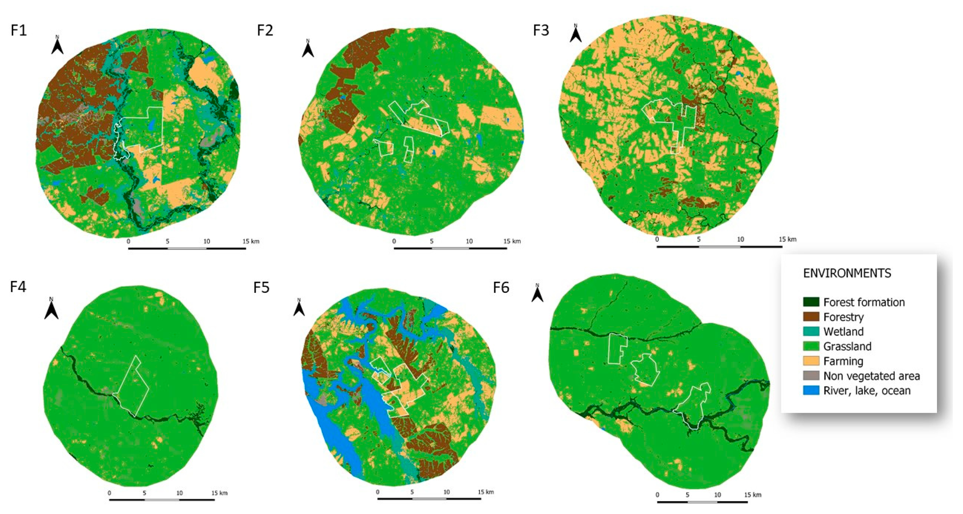
Habitat mapping around farms (Figure 4) shows the predominance of natural/semi-natural communities. In the case of farm 3, the farming area in the surroundings is important, and forestry is an important land use in the landscape of farm 1 (

Table A2. Landscape proportions of each farm (F).

Environment	F1	F2	F3	F4	F5	F6
Forest Formation	6.6	0.5	1.4	2.0	0.6	4.4
Forestry	19.4	6.9	4.6	0.3	12.0	0.4
Wetland	13.9	2.6	0.1	0.0	10.7	0.0
Grassland	44.7	76.4	62.7	95.1	48.1	92.0
Farming	12.6	12.9	30.8	1.2	13.7	2.0
Non Vegetated Area	2.3	0.5	0.4	1.4	1.3	0.9
River, Lake and Ocean	0.5	0.2	0.0	0.0	13.5	0.3

). The dominant environment in the landscape around all farms and the least fragmented is grassland (Table A2,

Table A3. Effective mesh size (km²) of farm landscapes. F: farm.

Environment	F1	F2	F3	F4	F5	F6
Forest Formation	0.080	0.00	0.0077	0.03	0.00	0.24
Forestry	12.979	2.79	0.0237	0.00	0.87	0.00
Wetland	1.406	0.01	0.0000	0.00	0.78	0.00
Grassland	32.232	351.62	140.7748	249.36	30.80	263.49
Farming	0.894	0.44	6.3827	0.00	0.50	0.02
Non Vegetated Area	0.016	0.00	0.0001	0.00	0.01	0.00
River, Lake and Ocean	0.002	0.00	0.0001	0.00	9.79	0.00

and

Table A4. Largest patch index of farm landscapes. F: farm.

Environment	F1	F2	F3	F4	F5	F6
Forest Formation	0.52	0.0675	0.297	0.5824	0.05	1.0684
Forestry	15.07	6.5284	0.340	0.0087	2.29	0.0085
Wetland	4.20	0.1614	0.008	0.0003	2.24	0.0037
Grassland	20.19	73.2178	50.718	55.4189	18.59	44.7041
Farming	2.83	1.9315	9.630	0.1083	1.95	0.3448
Non Vegetated Area	0.31	0.0250	0.009	0.0324	0.27	0.0500
River, Lake and Ocean	0.10	0.0768	0.037	0.0105	12.47	0.0356

).

The only identified element that could constitute an obstacle to the mobility of wildlife between habitats were fences, but most species of fauna can cross them without problem, with the exception of the Rhea americana (Greater Rhea). No measures were identified to overcome this obstacle on any farm.

4. Discussion

4.1. Habitat Protection and Habitat Change

These first groups of indicators include the regulatory framework and actions adopted by farmers for conservation. This is the result of the revision of local and national regulations, which in the case of Uruguay are easily available, and interviews with the farmers to learn about their action plans and measures taken towards conservation. Although in principle it does not seem to have practical difficulties, in each case of application around the world aspects of accessibility to official information and a clear regulatory framework may condition the result. The second aspect to consider is cultural or personal aspects that may limit the responses of farmers to questions about their actions and decision-making. In this sense, most of the information could be obtained without difficulty for the six study cases.

For most of the indicators in these groups (especially those that involved mapping and area calculation), GIS layers were created. This was the end product of several stages, starting with the clear definition of the study areas, then an inventory and delimitation of the different environments present on each farm, as well as their management units. The incorporation of existing information for the study areas, field validation, and the modeling of information obtained using other methodologies such as the Ecosystem Integrity Index [40] followed.

It should be noted that although validation and field work were necessary for almost all stages, both Uruguay and the region have a lot of open-access geographic information (satellite) that improves and facilitates work [36,64].

The maps made by Carrasco and Beretta [38] based on the USLE/RUSLE model (widely used in Uruguay for land use and management plans, mandatory in agricultural systems) [39] were very useful to identify the risk of soil loss by erosion in areas with different uses. To identify existing situations of degradation related more specifically to livestock management, the Ecosystem Integrity Index was a useful tool [40]. By evaluating various characteristics related to the components: vegetation structure, plant species, soil, and riparian zones, it allowed the collection of a large amount of information for various indicators and served to distinguish situations of degradation related to livestock management at the paddock level or related to the management of cultivated pastures destined for cattle feeding.

The indicator that was the most difficult to monitor was “Livestock density” since stocking rates and forage availability are very dynamic and variable measures over time. For this study, only average values were obtained for the farm and not for paddocks or environments, potentially hiding possible overgrazing situations. The carrying capacity calculated for the pastures was carried out in a very simplified way and based on bibliography due to the lack of particular data for each farm. Furthermore, the “safe load” reference is a general value and is not useful for this indicator, for which it is necessary or at least desirable to have more local data. The amount of forage that is produced on each farm and even in the different environments within the farm is variable (due to the hydric and thermal regimes, soil conditions, etc.) so the same stocking rate may imply a different supply of forage per animal and therefore different grazing intensities [69]. In this sense, Soca et al. [69] propose this as a tool to calculate the intensity of grazing, the control of the offer or level of forage allocation (kg of dry matter (DM) per 100 kg of live weight). This indicator is also very dynamic and variable at the paddock level and therefore difficult to measure. An approximation could be a satellite estimate of the net primary production (NPP) [70] divided by the average annual stocking rate recorded, if possible per paddock.

4.2. Wildlife Conservation

This assessment requires qualified specialists and extensive field work. Therefore, it requires a high degree of interdisciplinary work and relatively high economic costs, requiring a careful analysis of the scope and the necessary specialists.

Regarding the evaluation of the state of wild populations, in this study, the criterion of incorporating representative classes of different phyla for the animal and plant kingdoms was adopted. In this sense, vascular plants for the dominant habitat (native grasslands) in reference paddocks and a list of species and diversity of woody species in native forests were selected for the plant kingdom. In the animal kingdom, a representative of terrestrial vertebrates (birds) and a representative of terrestrial invertebrates (spiders) were selected. Although it is considered in another group of indicators (pollution and aquatic biodiversity), fish were incorporated as vertebrates to represent the aquatic ecosystem.

In relation to the protection of habitats for species with high conservation value, some of them have legal protection. In this sense, the Uruguayan Law prohibits logging (except for domestic use) and “any operation that threatens the survival of the native forest” without authorization of the Agriculture Ministry [68]. This seeks the conservation of natural forests. Regarding fauna, hunting, capture, or sacrifice of wild animals and legally protected species is prohibited [71].

4.2.1. Birds

Birds are a good model for studying the state of ecosystems because there are species that occupy all trophic levels. The high richness recorded is not surprising since 90 species of birds inhabit the Uruguayan grasslands, to which the forest inhabitants are added, a habitat that is normally present in the country’s farms (and was present in all the case studies). Of these species, several are considered priorities for conservation due to the significant decrease in their national population size, the low natural effective density of their populations, and the loss of habitat [72,73]. Brennan and Kuvlesky [74] have suggested the population decline suffered by most grassland birds in North America due to habitat loss highlights “a major conservation crisis”. In Europe, between 1970 and 2000, 70% of grassland birds and other agroecosystems’ “farmland birds” decreased in abundance [75], mainly due to agricultural intensification [76]. In the grasslands of the Río de la Plata, at least 22 species of birds that inhabit the pampas and campos are threatened, both on a regional and global scale, and many others have decreased their population size considerably [72,77,78]. Many of these species were recorded on the sampled farms.

With regards to the methodology for assessment, birds are mostly diurnal and have identifiable vocalization, which facilitates their detection. In this study, McKinnon lists [79] were selected because they are an efficient method for listing most of the species inhabiting a certain area, independently of the environment, with a reasonable approximation to the proportion of each species within the community. Additionally, it can be done by less skilled observers, although it probably requires additional time. The main disadvantage is that easily detected or less common species’ proportions will be overestimated [54], which happens especially if large lists are used. In our experience, the method turned out to be very efficient for the detection of a large number of species with a reasonable sampling effort. In this study, 15-species lists were used, which is a large number for environments where the density of birds is low, such as pastures. The use of 10-species lists could improve efficiency by reducing the time needed to finish each list and reducing the overestimation of the proportion of common species and the underestimation of rare ones.

In tropical zones where richness is high, the sampling efficiency for point counts and the bioacoustic method is high [80]. Other methods, such as line transects commonly used in extensive open habitats, are very effective at determining population densities, especially when distance sampling methods are used, but they require very capable observers and a large sampling effort if knowledge of the richness and diversity of large areas is wanted [54].

4.2.2. Spiders

Spiders were chosen because, as a mega-diverse group, they are excellent study models for evaluating environmental impacts. They are the seventh group in species richness within arthropods, with more than 50,000 species known worldwide [81], and they are found in almost all terrestrial ecosystems and are generalist predators that play a fundamental role as biological controllers of pests in agroecosystems, thus providing an important ecosystem service [82]. The results obtained confirm spiders as a very useful group as a model for conducting diversity surveys and evaluations in grassland environments, such as cattle ranches, as has already been mentioned in other studies [83,84]. Additionally, they are good study models for estimating biological diversity, as well as for conservation and environmental quality as bio-indicators [85]. In recent years, the importance of this group has increased from a biodiversity conservation point of view [86]. Even in Uruguay, there are already lists of priority arachnids [57], and in the samplings, species that are on these lists were found, generating more importance to the livestock grasslands of the region.

It is difficult to know which sampling technique is the most efficient and easiest to use in diversity survey studies such as those required in the LEAP guidelines. It could be considered that the use of complementary techniques, such as those used in this study (g-vac and pitfalls), allows for a broader panorama of the grassland spider community, recording ground and vegetation species. In this study, the g-vac method collected three times as many specimens and more than twice as many species as the pitfalls. These lower numbers in pitfall traps compared to other techniques were recorded in other inventory studies with spiders [87]. Furthermore, g-vac requires a much lower budget in time and money compared to pitfall traps [88,89]. The g-vac technique ensures that samples are not lost when taking them, since the pitfall traps are exposed to rain or the actions of animals. However, pitfall traps are highly recommended for diversity inventories [83], and this is because a large percentage of adults are obtained, it is a measure of individual activity, and it allows collection of spiders that live at ground level and are not recorded with other methods (for example, in this study the spiders of the Lycosidae family were collected almost entirely with pitfalls).

According to the rarefaction curves, the total number of samples used could be considered efficient for this type of diversity survey with minimal effort. If the number of samples is reduced in order to reduce costs and time, many species would be lost, since with half the samples, between 10 and 15 fewer species are recorded in some paddocks. When comparing the sampling dates, although the number of species increases when working in the four seasons, clearly the summer period is much more effective for carrying out surveys of spiders, and a greater number of species and individuals are obtained than in the colder dates.

With the results obtained, if shorter times and reducing economic costs were required, the recommendation is to carry out a survey only in the summer or on two dates in the spring and summer, with the g-vac technique that allows obtaining a large number of specimens and species in a short period of time.

Although some capture techniques, such as those used here, can be carried out by people without previous training or experience, the identification of specimens at the species level requires the participation of specialists in the subject [87].

A large number of specimens and species of spiders were obtained for this study. The diversity values were high compared to other ecosystems in the region [90,91]. Aglaoctenus lagotis (Lycosidae) and Mesabolivar tandilicus (Pholcidae) were recorded (Table S9), two species considered a priority for their conservation [57]. Both species were not recorded in large numbers, which may be due to the fact that the techniques used are not adequate to collect them due to their lifestyle. Mesabolivar tandilicus was found exclusively in native grasslands, which shows the importance of conserving these environments.

4.2.3. Herbaceous Species

The study of the flora and herbaceous vegetation of the native grasslands is essential since they are environmentally important and the main feeding source of the six farms in the study. Native grasslands are the dominant plant formation in Uruguay, occupying 66% of the national territory [34]. They reside within the Río de la Plata Grasslands, one of the most important temperate grassland regions in the world [92].

The sampled grasslands presented a great heterogeneity of communities and different strata. Livestock influences the conservation of grassland diversity since it can modify its structure and floristic composition [93,94]. Knowledge of the species that comprise the community is essential to determining grazing management strategies to prevent and control the degradation processes of this environment [95,96,97].

The heterogeneity of the environment at the local scale (even at the paddock level, such as those sampled) also contributes to the maintenance of the diversity of some faunal groups, such as soil invertebrates, by providing different niches and refuges [98,99].

Sampling native grassland herbaceous species in livestock production systems is complex and requires the support of specialists since most species are grazed, making their identification difficult.

Some of the surveys were carried out during the months of February and March, which is not the optimal time to carry out a characterization of the flora since many of the plant species are in a vegetative state or remain only in reserve structures. It is recommended to carry out the surveys from October to December, a period in which most of the species present reproductive structures that enable and facilitate their identification. Ideally, a survey would include sampling in both seasons, late spring/early summer and late summer/early fall, so as to coincide with the two big flowering peaks of plants in this region and therefore obtain a more complete record of all species present.

Being the basis of livestock feeding and therefore subject to grazing and animal selectivity, the diversity conservation of this stratum represents a challenge. The priority species for conservation were recorded at low frequencies. Any conservation strategy must consider aspects of palatability for livestock in addition to the ecological conditions that favor them.

4.2.4. Woody Species

Forests host most of the world’s terrestrial biodiversity [100]. Although Uruguay has a low forest area (about 5%) [34], these constitute the habitat for a large number of plant species (136 tree species, 150 shrub species, and 120 fern species have been identified) and animals (approximately 50% of mammal and bird species are linked to the forest) [101] and provide valuable ecosystem services such as climate regulation, carbon sequestration, water quality regulation, watershed conservation, etc. [100,101,102,103,104]. Riparian forests are the most abundant type and form a buffer strip along most of the country’s rivers and streams [101,105]. Forests also provide important services to production systems, such as refuges and shade for livestock [102,106].

To identify and reverse the causes of native forest deterioration and improve its quality, Uruguay joined the REDD+ initiative that emerged under the United Nations Framework Convention on Climate Change [107]. Among the many objectives of this initiative, the development of a protocol for the evaluation of native forest integrity is included. The REDD+ integrity assessment protocol was used for this study as it involves the evaluation of multiple attributes to obtain an approximation of the conservation status of native forests and allows the calculation of species diversity indices. It is also a valuable tool to detect evolution over time and changes due to management practices.

The richness of the studied farms is greater than what the transects were able to capture, probably due to the number of environmental variants in the microsites. Data recording during the application of the Ecosystem Integrity Index was complementary and generated a broader record of the farms’ woody species richness. Considering the proposed reference for interpretation of results [49], the richness, soil cover, and canopy cover are considered good. However, the average number of seedlings is variable within the farms, being good for farm 1 but intermediate for the rest of the farms. This is probably caused by the grazing effect, and it is a matter that must be addressed since it could affect the renewal of the forest. Livestock systems can generate impacts on native forests. Depending on management, cattle can alter these ecosystems by affecting species regeneration, reducing herbaceous vegetation, dispersing seeds of invasive exotic species, and generating erosion and soil compaction [106,108,109]. Likewise, it has been shown that measures such as the exclusion or control of livestock entry to forests by fences help to prevent these damages or improve the conservation status of these ecosystems [106].

Although the area of native forests in Uruguay has increased in recent years [110], they are undergoing degradation processes. Two of the biggest threats are invasion by exotic species and agricultural expansion [101].

In future work, an increase in the number of sampling points should be considered to capture the existing richness. In any case, one of the main objectives should be the evolution of the sites sampled over time in order to evaluate the effect of eventual interventions to improve the state of forests, not only in terms of richness and diversity but also in structure.

4.3. Invasive Species

Invasive alien species are one of the main threats to biodiversity, they cause extinctions, produce changes in the composition and functioning of ecosystems, cause economic losses, and impact human and animal health [111,112,113]. Some of these species were recorded in this work, such as Eragrostis plana and Gleditsia triacanthos.

A recent study by Olivera and Riaño [109] showed that approximately 2.6% of the native forest area in Uruguay is invaded by two of the most aggressive exotic species present in the country, Ligustrum lucidum and Gleditsia triacanthos.

Invasive exotic herbaceous and woody species threaten the diversity of grasslands and forests, and impact livestock productivity by reducing forage quality (low palatability) and/or quantity [102,114,115,116].

Although a low incidence of exotic species has been reported in Uruguayan grasslands with extensive uses [117], some hazardous invasive species were identified that represent a great risk to local species communities and populations and can cause important economic and ecological impacts for Uruguay and the region [109,116,118,119].

Livestock can contribute to the seed dispersal of invasive plant species [120,121], but through grazing management, it can play a dual role with respect to native grasslands invasions. Cattle generate direct damage to plants through consumption; also, the intensity of grazing influences local resource availability (space, water, light, nutrients, etc.) and can be used as a regulator of the competition processes in grassland plant communities (altering vegetation structure and species richness) [115,116,122]. Therefore, grazing management can favor or limit the availability of resources for invaders, and consequently be used as a control tool, as in the case of farm 5.

There were no problems in the identification of exotic invaders by specialists, especially with the fauna and flora surveys carried out previously, but the ease of identification of exotic invasive species by farmers depends on the taxonomic group, on the information obtained through campaigns of recognition and control of these species, and on the risk they represent for the production system.

Although some control measures were recorded, few of the invasive species identified were under a management plan with strategic actions, a systemic view, and multi-year planning. Managing biological invasions requires great effort and economic resources that not all farmers have or are willing to provide.

In general, producers recognized only the most important or aggressive invaders and controlled those that affect agricultural production, affecting direct use values (e.g., forage or crop production). The loss or alteration of indirect use values (regulating and supporting services, e.g., natural pest control, soil fertility, water purification, etc.) or non-market-based ecosystem services by invasive species is often overlooked or underappreciated because they are poorly understood [114].

It is important that producers know the invasive alien species present inside the farm as well as in the surroundings and can predict the impact or consequences of agricultural and livestock management decisions in order to prevent the invasion of their production systems (especially related to flora).

Regarding certain taxonomic groups or at scales that escape the control or prevention of farmers, it is also necessary, as mentioned by Fonseca [118], to establish coherent national and regional legislation and socio-environmental education on the subject.

4.4. Pollution and Aquatic Biodiversity

4.4.1. Water Quality

Water quality monitoring allowed us to assess the effect of land use [123,124] and detect differences between the streams studied and both seasons. The P concentration of the streams analyzed showed generally good water quality, with values lower than 25 µg P/L of total phosphorus (TP), which is the upper limit value in the current regulations [125]. This limit is rarely exceeded in systems of low intensity land use, such as extensive cattle ranching in Uruguay [126]. In the case of N, most of the sites also correspond to low-intensity land use systems [126]. Two streams presented values that can be considered as values corresponding to systems between low and high agricultural intensities (>700 µg/L) [124,126]. Therefore, it is necessary to pay special attention to the spatial and temporal variability of nitrogen in these systems. In addition, the same systems that presented elevated nitrogen concentrations in water also presented dissolved oxygen values that corresponded to hypoxia-anoxia values or supersaturation values. The first case represents evidence of a high organic matter load where decomposition processes outweigh oxygen production, and in the second case, an excessive production of oxygen by the primary producers [127]. These symptoms represent eutrophication processes, which in the case of land uses with low nutrient application may be due to direct access of livestock to watercourses, something that was observed in some of the sampled sites. This can occur particularly in cases of hypoxia and anoxia, where the entry of livestock, in addition to direct urine and feces, generates locally an important removal of sediments, making organic matter available in the water column with the consequent consumption of oxygen [128]. In addition, by increasing turbidity, the entry of light for primary producers is prevented, again favoring oxygen consumption. Situations of oxygen supersaturation correspond to systems with a high development of primary producers (mainly periphyton) due to the availability of nutrients and clear water [127]. The sampling strategy allowed us to see the importance of implementing the monitoring of physical-chemical parameters at different times of the year, in accordance with other high frequency monitoring strategies [123,124].

4.4.2. Fish Community

Fish play a fundamental role in the food web and functioning of inland water systems and can affect nutrient translocation and predator-prey interactions in all habitats, as they exhibit a great diversity of feeding modes and are generally the top predators within the aquatic system [129]. Moreover, the analysis of fish community biomass is considered a functional response of the system as well as an ecosystem service [130]. The monitoring system used in this work proved to be effective, allowing the capture of more than 40 species, including rare taxa, with the number of species observed exceeding 80% of the estimated number of species. The sampling strategy used has been previously validated when compared to monitoring systems that involve a greater sampling effort, so it generates a lower impact on the system [131]. Fish communities are used worldwide in biomonitoring programs to assess the effects of land use due to the existence of species that are sensitive or tolerant to changes in water quality and physical habitat modification [132]. In Uruguay, there is clear evidence of different types of fish communities’ responses to different land uses [130,133,134].

The systems analyzed presented a diversity of species similar to systems with low impacted land use [60,131]. The results of the performed monitoring, combining water quality and fish communities, showed coincidences between lower water quality and a deteriorated fish community, with low species richness and dominated by Cnesterodon decemmaculatus, a tolerant species and an indicator of environmental deterioration [130,133,134]. The coincidence between poor water quality and a deteriorated fish community indicates that the situation of environmental degradation has been maintained over time since disturbances at a specific moment in time do not generally affect the fish community.

Another relevant aspect to consider in the evaluations is the presence of priority species for conservation. In this study, the presence of priority species was observed in all the farms, indicating the importance of maintaining the diversity of these systems. On the other hand, it is important to mention that this list [135] should be updated since it is almost 10 years old and there have already been taxonomic revisions that have generated changes for our country (e.g., Hoplias malabaricus change to H. argentinensis), as well as descriptions of new species that, based on their restricted distribution and the interest of their use in aquarism, should be included as priority species (e.g., Gymnogeophagus peliochelynion).

4.5. Off-Farm Feed

Given the globalization of agricultural supply chains, the environmental effects of a livestock system can occur in multiple geographic areas [32]. The expansion of croplands for livestock feed purposes can encourage deforestation, the removal of wildlife habitats, and generate significant impacts on biodiversity and ecosystem services by the replacement of high conservation value environments [26,136,137,138].

In this sense, the engagement of livestock farmers (and other stakeholders) who use imported feed is necessary so that they can understand and be informed about the impacts generated by the products they buy in their place of origin [2]. However, foods produced outside the farm (such as salt, grains, or energy concentrates) in extensive systems in Uruguay, such as those studied, are generally nationally produced and used in low volumes with strategic objectives. They are used to cover the requirements of certain categories when their physiological demand is high and/or at times when the forage supply is low or of lower quality.

This indicator arises from the life cycle analysis methodology, that is, the impact generated on biodiversity by the production cycle of that food imported to the farm as an input. The most measurable indicator is the area assigned to the production of food, such as grains or fodder, which implies replacing the native community with a crop. In this case, an estimation of the impacted area could be assigned based on the average productivity (kg/ha) of each crop and the consumption of food (kg) of each farm.

For example, in the case of corn grain, which has an average yield of 6000 kg/ha in Uruguay [34], we could say that farm 2 affects 40.8 hectares dedicated to cultivation; but also, in this case, there are several considerations that make it difficult to assign an impact on biodiversity, for example, that it is a seasonal crop and therefore that area of land has another use for half the year (shared impact).

Another additional difficulty is when it comes to industrial by-products, such as the case of corn DDGS or rice bran. In these cases, the area could be counted according to the percentage that this by-product represents over the total grain. Another challenge for analysis is that the negative impact generated in the crop production area or the possible increase in the livestock stocking rate could be partially offset. This is because of the positive effect that the correct use of strategic supplementation can generate in the states of the native communities of grasslands [139,140].

Considering that the determination of the impact depends not only on the replaced area but also on how this crop contributes or does not contibute habitat to certain organisms, in the near future, a better approximation can be to have average EII values of the different crops in order to have a quantifiable measure of the impact on ecosystem integrity.

4.6. Landscape-Scale Conservation

Nowadays, there is a large and growing amount of open-access geographic information as well as tools with functions that facilitate the calculation of landscape metrics [35,64,65].This improves the efficiency of the planning, design, and management of ecosystems [141,142]. For this, it is necessary not only to analyze the structure of the landscape but also to understand how some organisms or agroecosystems interact with the surrounding landscape matrix [143,144,145].

There are many landscape metrics that allow the study of its structural patterns at different levels (patch, class, and landscape) [67,146]; the decision of which to include depends on the research objectives, the different aspects of the landscape structure to be analyzed, and their relationship with certain ecological processes of interest [112,119,143,147,148].

Based on a previous study of the heterogeneity and fragmentation of the temperate grasslands of South America [149] and the recommendations of the LEAP guidelines [2], for this work, three indices were chosen: landscape proportion, largest patch index, and effective mesh size [66,67].

Landscape proportion (LP) quantifies the number and relative area of different land uses [67]. It was the most basic and useful index to characterize the composition and heterogeneity of the studied areas. The largest patch index (LPI) measures the proportion of the total landscape area comprised by the largest patch of each class, providing a class-level measure of dominance [67]. The greatest advantage of these two indices is their ease of calculation, interpretation, and communication.

Effective mesh size (MESH) is a measure of the degree of landscape fragmentation that has the ability to detect structural differences (“MESH takes into account the patch size distribution of the corresponding class as well as the total landscape area comprised of that class”). This method is characterized by the advantages of being insensitive to the omission or addition of very small patches and for characterizing the subdivision of a landscape regardless of its size (being area-proportionately additive), which makes it effective when comparing the fragmentation of regions with different surfaces [66,67]. However, this index has the disadvantage of not being intuitive and easy to interpret.

The analysis using these indices made it possible to identify the heterogeneity in the composition and configuration of the landscape of which the studied farms are part. Productive activities generate changes in land use and land cover that can lead to the loss, modification, and fragmentation of habitats [150]. All this, together with the loss of connectivity, can impair the movement of individuals and matter in the ecosystem, generating problems for biodiversity and ecosystem services [87,151,152,153,154,155]. Changes in landscape configuration can also generate vulnerability to important degradation processes such as invasion by exotic species [112,119].

Despite the advance of agriculture, forestry, and some intensification strategies in the livestock sector (perennial and annual pastures), native grasslands continue to be the main environment and the feeding base of the activity that occupies most of the Uruguayan territory [34]. The six study farms and their surrounding landscape were representative of this situation. The main vegetation, in all cases, was native grassland, a class that also represented the greatest dominance in patch size and the least fragmentation evaluated through effective mesh size (Table A2, Table A3 and Table A4). In farms 2 to 6, the proportion of environments is very similar to that of the surrounding landscape. In farm 1 (forage base 100% native grassland), the proportion of substituted environments in the surrounding landscape amounts to more than 30%, with commercial forestation being the second most important and least fragmented land use.

Changes over time in these indicators provide important information on large-scale trends in habitat quantity and configuration in the landscape, and they can help to predict and prevent degradation processes associated with these changes.

5. Conclusions

The LEAP assessment guideline is a useful tool to both characterize the state of ecosystems under pastoral use and some specific components of their biodiversity and assess the interaction of the production system with the environment and plan management accordingly.

Some of the indicators recommended by the guide, especially those that include studies of groups of fauna and flora, can be very costly to carry out, in terms of time and money, as well as requiring the support of numerous specialists; therefore, it is necessary to have the appropriate amount of resources so that the studies are as complete and in-depth as possible.

It was possible to generate, for the case studies, the basic information for the set of indicators proposed in the LEAP guidelines, but they must be monitored over time to assess the consequences of management decisions.

In the cases studied, there was a high richness of the species evaluated, many of which are priorities for conservation, demonstrating the importance of maintaining native communities as habitats for wild species. Livestock systems that preserve a great proportion of the land cover as native grasslands and forests will allow the conservation of these environments, increasing their function as reservoirs of biodiversity. Emerging problems such as exotic species invasions are increasing, not only due to the impacts but also due to the low consideration of farmers.

Off-farm food utilization can have negative or positive effects inside the farms but also generate impacts in other places, which are difficult to measure.

The use of indicators, such as the EII, that synthesize a lot of information and give an idea of the state and potential functioning of the ecosystems can be a good strategy to maintain frequent monitoring and allow extending the periods for more expensive indicators.

Establishing regular biodiversity measurement protocols, such as the LEAP Guidelines, is essential to monitoring and maintaining real sustainable systems.

The implementation of the assessment of biodiversity at the local level (farm) is essential to be able to make practical decisions in the improvement of processes and also in the possibility of showing consumers the contributions of systems to conservation.

The main aims of this work are to help in the wider application of the guidelines by facilitating decisions about the methodology, necessary resources, and the necessity of developing a cooperation strategy between the agriculture sector and biodiversity researchers. Moreover, to show the importance of native grasslands-based livestock systems for biodiversity conservation.

References

1. Pimm, S.L.; Jenkins, C.N.; Abell, R.; Brooks, T.M.; Gittleman, J.L.; Joppa, L.N.; Raven, P.H.; Roberts, C.M.; Sexton, J.O. The Biodiversity of Species and Their Rates of Extinction, Distribution, and Protection. Science 2014, 344, 1246752. [Google Scholar] [CrossRef]
2. FAO. Biodiversity and the Livestock Sector—Guidelines for Quantitative Assessment; FAO: Rome, Italy, 2020; ISBN 978-92-5-132745-6. [Google Scholar]
3. Phelps, L.N.; Kaplan, J.O. Land Use for Animal Production in Global Change Studies: Defining and Characterizing a Framework. Glob. Chang. Biol. 2017, 23, 4457–4471. [Google Scholar] [CrossRef] [PubMed] [Green Version]
4. Lambin, E.F.; Geist, H.J.; Lepers, E. Dynamics of Land-Use and Land-Cover Change in Tropical Regions. Annu. Rev. Environ. Resour. 2003, 28, 205–241. [Google Scholar] [CrossRef] [Green Version]
5. Wassenaar, T.; Gerber, P.; Verburg, P.H.; Rosales, M.; Ibrahim, M.; Steinfeld, H. Projecting Land Use Changes in the Neotropics: The Geography of Pasture Expansion into Forest. Glob. Environ. Chang. 2007, 17, 86–104. [Google Scholar] [CrossRef]
6. Nepstad, D.; McGrath, D.; Stickler, C.; Alencar, A.; Azevedo, A.; Swette, B.; Bezerra, T.; DiGiano, M.; Shimada, J.; Seroa da Motta, R.; et al. Slowing Amazon Deforestation through Public Policy and Interventions in Beef and Soy Supply Chains. Science 2014, 344, 1118–1123. [Google Scholar] [CrossRef]
7. Bignal, E.M.; McCracken, D.I. The Nature Conservation Value of European Traditional Farming Systems. Environ. Rev. 2000, 8, 149–171. [Google Scholar] [CrossRef]
8. Atkinson, P.W.; Fuller, R.J.; Vickery, J.A. Large-Scale Patterns of Summer and Winter Bird Distribution in Relation to Farmland Type in England and Wales. Ecography 2002, 25, 466–480. [Google Scholar] [CrossRef]
9. Laiolo, P.; Dondero, F.; Ciliento, E.; Rolando, A. Consequences of Pastoral Abandonment for the Structure and Diversity of the Alpine Avifauna. J. Appl. Ecol. 2004, 41, 294–304. [Google Scholar] [CrossRef]
10. Rook, A.J.; Dumont, B.; Isselstein, J.; Osoro, K.; WallisDeVries, M.F.; Parente, G.; Mills, J. Matching Type of Livestock to Desired Biodiversity Outcomes in Pastures—A Review. Biol. Conserv. 2004, 119, 137–150. [Google Scholar] [CrossRef]
11. Augustine, D.J.; Derner, J.D.; Fernández-Giménez, M.E.; Porensky, L.M.; Wilmer, H.; Briske, D.D. Adaptive, Multipaddock Rotational Grazing Management: A Ranch-Scale Assessment of Effects on Vegetation and Livestock Performance in Semiarid Rangeland. Rangel. Ecol. Manag. 2020, 73, 796–810. [Google Scholar] [CrossRef]
12. Gonzalez Fischer, C.; Bilenca, D. Can We Produce More Beef without Increasing Its Environmental Impact? Argentina as a Case Study. Perspect. Ecol. Conserv. 2020, 18, 1–11. [Google Scholar] [CrossRef]
13. Tyrrell, P.; Russell, S.; Western, D. Seasonal Movements of Wildlife and Livestock in a Heterogenous Pastoral Landscape: Implications for Coexistence and Community Based Conservation. Glob. Ecol. Conserv. 2017, 12, 59–72. [Google Scholar] [CrossRef]
14. Young, T.P.; Porensky, L.M.; Riginos, C.; Veblen, K.E.; Odadi, W.O.; Kimuyu, D.M.; Charles, G.K.; Young, H.S. Relationships Between Cattle and Biodiversity in Multiuse Landscape Revealed by Kenya Long-Term Exclosure Experiment. Rangel. Ecol. Manag. 2018, 71, 281–291. [Google Scholar] [CrossRef]
15. Neilly, H.; O’Reagain, P.; Vanderwal, J.; Schwarzkopf, L. Profitable and Sustainable Cattle Grazing Strategies Support Reptiles in Tropical Savanna Rangeland. Rangel. Ecol. Manag. 2018, 71, 205–212. [Google Scholar] [CrossRef]
16. Dominati, E.J.; Mackay, A.D.; Rendel, J.M.; Wall, A.; Norton, D.A.; Pannell, J.; Devantier, B. Farm Scale Assessment of the Impacts of Biodiversity Enhancement on the Financial and Environmental Performance of Mixed Livestock Farms in New Zealand. Agric. Syst. 2021, 187, 103007. [Google Scholar] [CrossRef]
17. Collins, S.L.; Knapp, A.K.; Briggs, J.M.; Blair, J.M.; Steinauer, E.M. Modulation of Diversity by Grazing and Mowing in Native Tallgrass Prairie. Science 1998, 280, 745–747. [Google Scholar] [CrossRef]
18. Manzano, P.; Malo, J.E. Extreme Long-Distance Seed Dispersal via Sheep. Front. Ecol. Environ. 2006, 4, 244–248. [Google Scholar] [CrossRef]
19. Pulido, M.; Schnabel, S.; Lavado Contador, J.F.; Lozano-Parra, J.; González, F. The Impact of Heavy Grazing on Soil Quality and Pasture Production in Rangelands of SW Spain: Soil Quality and Pasture Production in Rangelands of SW Spain. Land Degrad. Dev. 2018, 29, 219–230. [Google Scholar] [CrossRef]
20. Zhan, T.; Zhang, Z.; Sun, J.; Liu, M.; Zhang, X.; Peng, F.; Tsunekawa, A.; Zhou, H.; Gou, X.; Fu, S. Meta-Analysis Demonstrating That Moderate Grazing Can Improve the Soil Quality across China’s Grassland Ecosystems. Appl. Soil Ecol. 2020, 147, 103438. [Google Scholar] [CrossRef]
21. Zhang, R.; Yeh, E.T.; Tan, S. Marketization Induced Overgrazing: The Political Ecology of Neoliberal Pastoral Policies in Inner Mongolia. J. Rural Stud. 2021, 86, 309–317. [Google Scholar] [CrossRef]
22. Bouwman, A.F.; Beusen, A.H.W.; Billen, G. Human Alteration of the Global Nitrogen and Phosphorus Soil Balances for the Period 1970–2050: Nitrogen and Phosphorus Soil Balances. Glob. Biogeochem. Cycles 2009, 23, GB0A04. [Google Scholar] [CrossRef]
23. Bai, Z.H.; Ma, L.; Qin, W.; Chen, Q.; Oenema, O.; Zhang, F.S. Changes in Pig Production in China and Their Effects on Nitrogen and Phosphorus Use and Losses. Environ. Sci. Technol. 2014, 48, 12742–12749. [Google Scholar] [CrossRef] [PubMed]
24. Vörösmarty, C.J.; McIntyre, P.B.; Gessner, M.O.; Dudgeon, D.; Prusevich, A.; Green, P.; Glidden, S.; Bunn, S.E.; Sullivan, C.A.; Liermann, C.R.; et al. Global Threats to Human Water Security and River Biodiversity. Nature 2010, 467, 555–561. [Google Scholar] [CrossRef] [PubMed] [Green Version]
25. Clark, C.M.; Cleland, E.E.; Collins, S.L.; Fargione, J.E.; Gough, L.; Gross, K.L.; Pennings, S.C.; Suding, K.N.; Grace, J.B. Environmental and Plant Community Determinants of Species Loss Following Nitrogen Enrichment. Ecol Lett. 2007, 10, 596–607. [Google Scholar] [CrossRef]
26. Millennium Ecosystem Assessment. Ecosystems and Human Well-Being: Biodiversity Synthesis; World Resources Institute: Washington, DC, USA, 2005. [Google Scholar]
27. Teillard, F.; Anton, A.; Dumont, B.; Finn, J.A.; Henry, B.; Souza, D.M.; Manzano, P.; Milà i Canals, L.; Phelps, C.; Said, M.; et al. A Review of Indicators and Methods to Assess Biodiversity—Application to Livestock Production at Global Scale. Livestock Environmental Assessment and Performance (LEAP) Partnership; FAO: Rome, Italy, 2016. [Google Scholar]
28. Cleland, E.E. Biodiversity and Ecosystem Stability. Nat. Educ. Knowl. 2011, 3, 14. [Google Scholar]
29. Kok, A.; Oostvogels, V.J.; de Olde, E.M.; Ripoll-Bosch, R. Balancing Biodiversity and Agriculture: Conservation Scenarios for the Dutch Dairy Sector. Agric. Ecosyst. Environ. 2020, 302, 107103. [Google Scholar] [CrossRef]
30. FAO Leap at a Glance 2017. Available online: https://www.fao.org/3/i7804e/i7804e.pdf (accessed on 5 November 2022).
31. FAO Science-Based Approach|Livestock Environmental Assessment and Performance (LEAP) Partnership|Food and Agriculture Organization of the United Nations. Available online: https://www.fao.org/partnerships/leap/overview/science-based-approach/en/ (accessed on 28 November 2022).
32. Teillard, F.; Maia de Souza, D.; Thoma, G.; Gerber, P.J.; Finn, J.A. What Does Life-Cycle Assessment of Agricultural Products Need for More Meaningful Inclusion of Biodiversity? J. Appl. Ecol. 2016, 53, 1422–1429. [Google Scholar] [CrossRef] [Green Version]
33. Jeanneret, P.; Baumgartner, D.U.; Freiermuth Knuchel, R.; Koch, B.; Gaillard, G. An Expert System for Integrating Biodiversity into Agricultural Life-Cycle Assessment. Ecol. Indic. 2014, 46, 224–231. [Google Scholar] [CrossRef]
34. MGAP. DIEA (Ministerio de Ganadería, Agricultura y Pesca. Dirección de Investigaciones Estadísticas Agropecuarias, UY) Anuario Estadístico Agropecuario. 2020. Available online: https://www.gub.uy/ministerio-ganaderia-agricultura-pesca/datos-y-estadisticas/estadisticas/anuario-estadistico-agropecuario-2020 (accessed on 26 September 2022).
35. QGIS Development Team QGIS Geographic Information System 2021. Available online: https://qgis.org/es/site/forusers/download.html (accessed on 5 November 2022).
36. IDEUY. Available online: https://visualizador.ide.uy/ideuy/core/load_public_project/ideuy/ (accessed on 6 October 2022).
37. MGAP (Ministerio de Ganadería, Agricultura y Pesca, UY) Nueva Cartografía de Pastizales del Uruguay. Available online: https://www.gub.uy/ministerio-ganaderia-agricultura-pesca/politicas-y-gestion/nueva-cartografia-pastizales-del-uruguay (accessed on 6 October 2022).
38. Carrasco-Letelie, L.; Beretta-Blanco, A. Erosión Hídrica Del Suelo Estimada Para 99 Cuencas Uruguayas. Cienc. Investig. Agrar. 2017, 44, 184–194. [Google Scholar] [CrossRef] [Green Version]
39. García Préchac, F.; Terra, J.; Sawchik, J.; Bidegain, M.P. Mejora de las estimaciones con USLE/RUSLE empleando resultados de parcelas de escurrimiento para considerar el efecto del agua del suelo. Agrociencia Urug. 2017, 21, 100–104. [Google Scholar]
40. Blumetto, O.; Castagna, A.; Cardozo, G.; García, F.; Tiscornia, G.; Ruggia, A.; Scarlato, S.; Albicette, M.M.; Aguerre, V.; Albin, A. Ecosystem Integrity Index, an Innovative Environmental Evaluation Tool for Agricultural Production Systems. Ecol. Indic. 2019, 101, 725–733. [Google Scholar] [CrossRef]
41. Saravia, A.; César, D.; Montes, E.; Taranto, V.; Pereira, M. Manejo Del Rodeo de Cría Sobre Campo Natural; Plan Agropecuario: Montevideo, Uruguay, 2011. [Google Scholar]
42. Leborgne, R. Antecedentes Técnicos y Metodología Para Presupuestación En Establecimientos Lecheros; 2o Edición Corregida; Hemisferio Sur: Buenos Aires, Argentina, 2008. [Google Scholar]
43. Irigoyen, A. Presupuestación Forrajera; Plan Agropecuario: Montevideo, Uruguay, 2011. [Google Scholar]
44. Lezama, F.; Pereira, M.; Altesor, A.; Paruelo, J.M. ¿Cuán Heterogéneos Son Los Pastizales Naturales En Uruguay? In Bases Ecológicas y Tecnológicas para el Manejo de Pastizales II; Altesor, A., López-Mársico, L., Paruelo, J.M., Eds.; FPTA, INIA: Montevideo, Uruguay, 2019; pp. 15–26. [Google Scholar]
45. Dengler, J.; Chytrý, M.; Ewald, J. Phytosociology. In Encyclopedia of Ecology; Elsevier: Amsterdam, The Netherlands, 2008; pp. 2767–2779. ISBN 978-0-08-045405-4. [Google Scholar]
46. Braun-Blanquet, J. Sociología Vegetal. Estudio de Las Comunidades Vegetales; ACME Agency: Buenos Aires, Argentina, 1950. [Google Scholar]
47. Zuloaga, F.O.; Belgrano, M.J.; Zanotti, C.A. Actualización del catálogo de las plantas vasculares del cono sur. Darwiniana Nueva Ser. 2019, 7, 208–278. [Google Scholar] [CrossRef]
48. Raunkiaer, C. The Life Forms of Plants and Statistical Plant Geography; Being the Collected Papers of C. Raunkiaer; Clarendon Press: Oxford, UK, 1934. [Google Scholar]
49. Vaz, P.; Carabio, M. Subproducto 2: Indicadores del Estado de Conservacióndel Bosque Nativo. Producto 5: Estado Deconservación del Bosque; Vida Silvestre Uruguay, Convenio INIA-REDD+: Montevideo, Uruguay, 2020. [Google Scholar]
50. Shannon, C.; Weaver, W. The Mathematical Theory of Communication, 1st ed.; The University of Illinois Press: Champaign, IL, USA, 1964. [Google Scholar]
51. McCravy, K. A Review of Sampling and Monitoring Methods for Beneficial Arthropods in Agroecosystems. Insects 2018, 9, 170. [Google Scholar] [CrossRef] [PubMed] [Green Version]
52. Colwell, R.K. Statistical Estimation of Species Richness and Shared Species from Samples (EstimateS); University of Colorado: Boulder, CO, USA, 2013. [Google Scholar]
53. Di Rienzo, J.A.; Casanoves, F.; Balzarini, M.G.; Gonzalez, L.; Tablada, M.; Robledo, C.W. Infostat—Software Estadístico. 2016. Available online: https://www.infostat.com.ar/ (accessed on 5 November 2022).
54. Gibbons, D.W.; Gregory, R.D. Birds. In Ecological Census Techniques, 2nd ed.; Sutherland, W.J., Ed.; Cambridge University Press: Cambridge, UK, 2006; pp. 308–350. [Google Scholar]
55. Bojorges Baños, J.C. Riqueza de Especies de Aves: Propuestas Metodológicas Para Su Evaluación y Estimación. Cienc. Mar 2006, 30, 59–64. [Google Scholar]
56. Soutullo, A.; Clavijo, C.; Martínez-Lanfranco, J.A. (Eds.) Especies Prioritarias para la Conservación en Uruguay: Vertebrados, Moluscos Continentales y Plantas Vasculares: Antecedentes, Oportunidades y Desafíos, Primera ed.; SNAP/DINAMA/MVOTMA y DICYT/MEC: Montevideo, Uruguay, 2013; ISBN 978-9974-8259-7-0. [Google Scholar]
57. Ghione, S.; Coelho, L.; Costa, F.G.; García, L.F.; González, M.; Jorge, C.; Laborda, Á.; de Oca, L.M.; Pérez-Miles, F.; Postiglioni, R.; et al. Arácnidos prioritarios para la conservación en uruguay. Boletín de la Sociedad Zoológica del Uruguay 2017, 26, 1–8. [Google Scholar] [CrossRef]
58. Brazeiro, A.; Bresciano, D.; Brugnoli, E.; Iturburu, M. Especies Exóticas Invasoras de Uruguay: Distribución, Impactos Socioambientales y Estrategias de Gestión; Primera; RETEMA-UdelaR, CEEI-Ministerio de Ambiente: Montevideo, Uruguay, 2021. [Google Scholar]
59. Proyecto REDD+ Uruguay. Monitoreo de Especies Exóticas Invasoras del Bosque Nativo de Uruguay Mediante Sensoramiento Remoto; Ministerio de Ganadería, Agricultura y Pesca—Ministerio de Vivienda, Ordenamiento Territorial y Medio Ambiente: Montevideo, Uruguay, 2020.
60. Teixeira-de Mello, F.; Kristensen, E.A.; Meerhoff, M.; González-Bergonzoni, I.; Baattrup-Pedersen, A.; Iglesias, C.; Kristensen, P.B.; Mazzeo, N.; Jeppesen, E. Monitoring Fish Communities in Wadeable Lowland Streams: Comparing the Efficiency of Electrofishing Methods at Contrasting Fish Assemblages. Environ. Monit Assess 2014, 186, 1665–1677. [Google Scholar] [CrossRef]
61. Chao, A.; Gotelli, N.J.; Hsieh, T.C.; Sander, E.L.; Ma, K.H.; Colwell, R.K.; Ellison, A.M. Rarefaction and Extrapolation with Hill Numbers: A Framework for Sampling and Estimation in Species Diversity Studies. Ecol. Monogr. 2014, 84, 45–67. [Google Scholar] [CrossRef] [Green Version]
62. Hsieh, T.C.; Ma, K.H.; Chao, A. INEXT: An R Package for Rarefaction and Extrapolation of Species Diversity (Hill Numbers). Methods Ecol. Evol. 2016, 7, 1451–1456. [Google Scholar] [CrossRef]
63. R Core Team. R: The R Project for Statistical Computing; R Foundation for Statistical Computing: Vienna, Austria, 2020. [Google Scholar]
64. MapBiomas Pampa. Sudamericano Project Collection 1 of the Annual Pampa Coverage and Land Use Series. Available online: https://plataforma.pampa.mapbiomas.org/ (accessed on 23 September 2022).
65. Jung, M. LecoS—A Python Plugin for Automated Landscape Ecology Analysis. Ecol. Inform. 2016, 31, 18–21. [Google Scholar] [CrossRef]
66. Jaeger, J.A.G. Landscape Division, Splitting Index, and Effective Mesh Size: New Measures of Landscape Fragmentation. Landsc. Ecol. 2000, 15, 115–130. [Google Scholar] [CrossRef]
67. McGarigal, K.S.; Cushman, S.; Neel, M.; Ene, E. FRAGSTATS: Spatial Pattern Analysis Program for Categorical Maps. 2002. Available online: https://www.researchgate.net/profile/Samuel-Cushman-2/publication/259011515_FRAGSTATS_Spatial_pattern_analysis_program_for_categorical_maps/links/564217ea08aebaaea1f8b8dd/FRAGSTATS-Spatial-pattern-analysis-program-for-categorical-maps.pdf (accessed on 5 November 2022).
68. Law N° 15939. Available online: https://www.impo.com.uy/bases/leyes/15939-1987 (accessed on 23 September 2022).
69. Soca, P.; Espasandín, A.; Carriquiry, M. Efecto de la Oferta de Forraje y Grupo Genético de las Vacas Sobre la Productividad y Sostenibilidad de la Cría Vacuna en Campo Natural; INIA: Montevideo, Uruguay, 2013; p. 88. [Google Scholar]
70. Baeza, S.; Lezama, F.; Piñeiro, G.; Altesor, A.; Paruelo, J.M. Spatial Variability of Above-Ground Net Primary Production in Uruguayan Grasslands: A Remote Sensing Approach. Appl. Veg. Sci. 2010, 13, 72–85. [Google Scholar] [CrossRef]
71. Law N° 18471. Available online: https://www.impo.com.uy/bases/leyes/18471-2009 (accessed on 23 September 2022).
72. Azpiroz, A.B.; Isacch, J.P.; Dias, R.A.; Di Giacomo, A.S.; Fontana, C.S.; Palarea, C.M. Ecology and Conservation of Grassland Birds in Southeastern South America: A Review. J. Field Ornithol. 2012, 83, 217–246. [Google Scholar] [CrossRef]
73. Aldabe, J.; Arballo, E.; Caballero-Sadi, D.; Claramunt, S.; Cravino, J.; Rocca, P. Aves. In Especies Prioritarias para la Conservación en Uruguay. Vertebrados, Moluscos Continentales y Plantas Vasculares; Soutullo, A., Clavijo, C., Martínez-Lanfranco, J., Eds.; SNAP/DINAMA/MVOTMA y DICYT/MEC: Montevideo, Uruguay, 2013; pp. 149–173. [Google Scholar]
74. Brennan, L.A.; Kuvlesky, W.P. North American grassland birds: An unfolding conservation crisis? Wild 2005, 69, 1–13. [Google Scholar] [CrossRef]
75. Donald, P.F.; Sanderson, F.J.; Burfield, I.J.; van Bommel, F.P.J. Further Evidence of Continent-Wide Impacts of Agricultural Intensification on European Farmland Birds, 1990–2000. Agric. Ecosyst. Environ. 2006, 116, 189–196. [Google Scholar] [CrossRef]
76. Donald, P.F.; Green, R.E.; Heath, M.F. Agricultural Intensification and the Collapse of Europe’s Farmland Bird Populations. Proc. R. Soc. Lond. Ser. B Biol. Sci. 2001, 268, 25–29. [Google Scholar] [CrossRef] [Green Version]
77. Bilenca, D.; Miñarro, F. Identificación de Áreas Valiosas de Pastizal (AVPs) En Las Pampas y Campos de Argentina, Uruguay y Sur de Brasil; Fundación Vida Silvestre Argentina: Buenos Aires, Argentina, 2004. [Google Scholar]
78. BirdLife International. State of the World’s Birds. Available online: https://issuu.com/birdlife-international/docs/sowb_2018_english_for_web (accessed on 26 September 2022).
79. McKinnon, J.; Phillips, K. A Field Guide to the Birds of Borneo, Sumatra, Java and Bali; Oxford University Press: Oxford, UK, 1993. [Google Scholar]
80. Suárez-García, O.; González-García, F.; Celis-Murillo, A. Understanding the complementarity of two survey methods in the study of bird communities during the breeding season in a tropical cloud forest. Rev. Mex. Biodivers. 2017, 88, 880–887. [Google Scholar] [CrossRef]
81. World Spider Catalog. World Spider Catalog. Version 23.5; Natural History Museum Bern: Bern, Switzerland, 2022. [Google Scholar]
82. Michalko, R.; Pekár, S.; Dul’a, M.; Entling, M.H. Global Patterns in the Biocontrol Efficacy of Spiders: A Meta-Analysis. Glob. Ecol. Biogeogr. 2019, 28, 1366–1378. [Google Scholar] [CrossRef]
83. Cardoso, P.; Scharff, N.; Gaspar, C.; Henriques, S.S.; Carvalho, R.; Castro, P.H.; Schmidt, J.B.; Silva, I.; Szüts, T.; De Castro, A.; et al. Rapid Biodiversity Assessment of Spiders (Araneae) Using Semi-Quantitative Sampling: A Case Study in a Mediterranean Forest. Insect Conserv. Divers. 2008, 1, 71–84. [Google Scholar] [CrossRef]
84. Cardoso, P. Standardization and Optimization of Arthropod Inventories—The Case of Iberian Spiders. Biodivers. Conserv. 2009, 18, 3949. [Google Scholar] [CrossRef]
85. Birkhofer, K.; Entling, M.H.; Lubin, Y. Agroecology: Trait Composition, Spatial Relationships, Trophic Interactions. In Spider Research in the 21st Century: Trends & Perspectives; Penney, D., Ed.; Siri Scientific Press: Manchester, UK, 2013; pp. 200–228. [Google Scholar]
86. Milano, F.; Blick, T.; Cardoso, P.; Chatzaki, M.; Fukushima, C.S.; Gajdoš, P.; Gibbons, A.T.; Henriques, S.; Macías-Hernández, N.; Mammola, S.; et al. Spider Conservation in Europe: A Review. Biol. Conserv. 2021, 256, 109020. [Google Scholar] [CrossRef]
87. Haddad, C.R. Undergraduate Entomology Field Excursions Are a Valuable Source of Biodiversity Data: A Case for Spider (Araneae) Bycatches in Ecological Studies. Biodivers. Conserv. 2021, 30, 4199–4222. [Google Scholar] [CrossRef] [PubMed]
88. Stewart, A.J.A.; Wright, A.F. A New Inexpensive Suction Apparatus for Sampling Arthropods in Grassland. Ecol. Entomol. 1995, 20, 98–102. [Google Scholar] [CrossRef]
89. Brennan, K.E.C.; Majer, J.D.; Moir, M.L. Refining sampling protocols for inventorying invertebrate biodiversity: Influence of drift-fence length and pitfall trap diameter on spiders. ARAC 2005, 33, 681–702. [Google Scholar] [CrossRef]
90. Simó, M.; Núñez, M.; Ojeda, L.; Laborda, Á.; Queirolo, D. Knowing the Biological Linkage: Spider Composition and Guilds in a Hill Range of Northern Uruguay. Boletín de la Sociedad Zoológica del Uruguay 2015, 24, 117–129. [Google Scholar]
91. Laborda, Á.; de Oca, L.M.; Pérez-Miles, F.; Useta, G.; Simó, M. The Spider Fauna from Uruguay River Islands: Understanding Its Role in a Biological Corridor. Biodivers. Data J. 2018, 6, e27319. [Google Scholar] [CrossRef] [PubMed] [Green Version]
92. Paruelo, J.M.; Jobbágy, E.G.; Oesterheld, M.; Golluscio, R.; Aguiar, M. The Grasslands and Steppes of Patagonia and the Río de La Plata Plains. In The Physical Geography of South America; Veblen, T.T., Young, K.R., Orme, A.R., Eds.; Oxford University Press: Oxford, UK, 2007; pp. 232–248. [Google Scholar]
93. Hayes, G.F.; Holl, K.D. Cattle Grazing Impacts on Annual Forbs and Vegetation Composition of Mesic Grasslands in California. Conserv. Biol. 2003, 17, 1694–1702. [Google Scholar] [CrossRef]
94. Altesor, A.; Oesterheld, M.; Leoni, E.; Lezama, F.; Rodríguez, C. Effect of Grazing on Community Structure and Productivity of a Uruguayan Grassland. Plant Ecol. 2005, 179, 83–91. [Google Scholar] [CrossRef]
95. Dorrough, J.; Yen, A.; Turner, V.; Clark, S.G.; Crosthwaite, J.; Hirth, J.R. Livestock Grazing Management and Biodiversity Conservation in Australian Temperate Grassy Landscapes. Aust. J. Agric. Res. 2004, 55, 279–295. [Google Scholar] [CrossRef] [Green Version]
96. Paruelo, J.M.; Golluscio, R.A.; Guerschman, J.P.; Cesa, A.; Jouve, V.V.; Garbulsky, M.F. Regional Scale Relationships between Ecosystem Structure and Functioning: The Case of the Patagonian Steppes. Glob. Ecol. Biogeogr. 2004, 13, 385–395. [Google Scholar] [CrossRef]
97. Modernel, P.; Rossing, W.A.H.; Corbeels, M.; Dogliotti, S.; Picasso, V.; Tittonell, P. Land Use Change and Ecosystem Service Provision in Pampas and Campos Grasslands of Southern South America. Environ. Res. Lett. 2016, 11, 113002. [Google Scholar] [CrossRef]
98. Vanbergen, A.J.; Watt, A.D.; Mitchell, R.; Truscott, A.-M.; Palmer, S.C.F.; Ivits, E.; Eggleton, P.; Jones, T.H.; Sousa, J.P. Scale-Specific Correlations between Habitat Heterogeneity and Soil Fauna Diversity along a Landscape Structure Gradient. Oecologia 2007, 153, 713–725. [Google Scholar] [CrossRef] [PubMed]
99. Aisen, S.; Werenkraut, V.; Márquez, M.E.G.; Ramírez, M.J.; Ruggiero, A. Environmental Heterogeneity, Not Distance, Structures Montane Epigaeic Spider Assemblages in North-Western Patagonia (Argentina). J. Insect Conserv. 2017, 21, 951–962. [Google Scholar] [CrossRef]
100. FAO and UNEP. The State of the World’s Forests 2020: Forests, Biodiversity and People; The State of the World’s Forests (SOFO); FAO and UNEP: Rome, Italy, 2020; ISBN 978-92-5-132419-6. [Google Scholar]
101. MGAP. Estrategia Nacional de Bosque Nativo, Primera ed.; Tradinco S.A: Montevideo, Uruguay, 2018. [Google Scholar]
102. Carrere, R. Monte Indígena: Mucho Más Que un Conjunto de Árboles, Primera ed.; Editorial Nordan y Brecha: Montevideo, Uruguay, 2001. [Google Scholar]
103. Anbumozhi, V.; Radhakrishnan, J.; Yamaji, E. Impact of Riparian Buffer Zones on Water Quality and Associated Management Considerations. Ecol. Eng. 2005, 24, 517–523. [Google Scholar] [CrossRef]
104. Lara, A.; Little, C.; Urrutia, R.; McPhee, J.; Álvarez-Garretón, C.; Oyarzún, C.; Soto, D.; Donoso, P.; Nahuelhual, L.; Pino, M.; et al. Assessment of Ecosystem Services as an Opportunity for the Conservation and Management of Native Forests in Chile. For. Ecol. Manag. 2009, 258, 415–424. [Google Scholar] [CrossRef]
105. Bernardi, R.; Buddeberg, M.; Arim, M.; Holmgren, M. Forests Expand as Livestock Pressure Declines in Subtropical South America. Ecol. Soc. 2019, 24, 19. [Google Scholar] [CrossRef] [Green Version]
106. Etchebarne, V.; Brazeiro, A. Effects of Livestock Exclusion in Forests of Uruguay: Soil Condition and Tree Regeneration. For. Ecol. Manag. 2016, 362, 120–129. [Google Scholar] [CrossRef]
107. Machín, I.; Ciganda, V.; Martino, D.; Gasparri, N.; Etchebarne Palla, V.; Lima, I.; González, I.; Paruelo, J. Bosque Nativo, Producción Agropecuaria y Cambio Climático: Proyecto REDD+; Revista INIA Nº 61; INIA: Montevideo, Uruguay, 2020; pp. 99–102. [Google Scholar]
108. Mazzini, F.; Relva, M.A.; Malizia, L.R. Impacts of Domestic Cattle on Forest and Woody Ecosystems in Southern South America. Plant Ecol. 2018, 219, 913–925. [Google Scholar] [CrossRef]
109. Olivera, J.M.; Riaño, M.E. Remote Sensing of Invasive Alien Woody Species in Uruguayan Native Forests. Agrociencia Urug. 2022, 26, e653. [Google Scholar] [CrossRef]
110. FAO. Atlas de Cobertura del Suelo de Uruguay, 1st ed.; DINOT, FAO: Montevideo, Uruguay, 2015; ISBN 978-92-5-308711-2. [Google Scholar]
111. Pimentel, D.; McNair, S.; Janecka, J.; Wightman, J.; Simmonds, C.; O’Connell, C.; Wong, E.; Russel, L.; Zern, J.; Aquino, T.; et al. Economic and Environmental Threats of Alien Plant, Animal, and Microbe Invasions. Agric. Ecosyst. Environ. 2001, 84, 1–20. [Google Scholar] [CrossRef]
112. Hobbs, R.J. Synergisms among Habitat Fragmentation, Livestock Grazing, and Biotic Invasions in Southwestern Australia. Conserv. Biol. 2001, 15, 1522–1528. [Google Scholar] [CrossRef]
113. Simberloff, D.; Martin, J.-L.; Genovesi, P.; Maris, V.; Wardle, D.A.; Aronson, J.; Courchamp, F.; Galil, B.; García-Berthou, E.; Pascal, M.; et al. Impacts of Biological Invasions: What’s What and the Way Forward. Trends Ecol. Evol. 2013, 28, 58–66. [Google Scholar] [CrossRef] [PubMed] [Green Version]
114. Charles, H.; Dukes, J.S. Impacts of Invasive Species on Ecosystem Services. In Biological Invasions; Ecological Studies; Nentwig, W., Ed.; Springer: Berlin/Heidelberg, Germany, 2007; pp. 217–237. ISBN 978-3-540-36920-2. [Google Scholar]
115. Baggio, R.; de Medeiros, R.B.; Focht, T.; Boavista, L.R.; Pillar, V.D.; Müller, S.C. Effects of Initial Disturbances and Grazing Regime on Native Grassland Invasion by Eragrostis Plana in Southern Brazil. Perspect. Ecol. Conserv. 2018, 16, 158–165. [Google Scholar] [CrossRef]
116. Wijayabandara, K.; Campbell, S.; Vitelli, J.; Shabbir, A.; Adkins, S. Review of the Biology, Distribution, and Management of the Invasive Fireweed (Senecio Madagascariensis Poir). Plants 2022, 11, 107. [Google Scholar] [CrossRef] [PubMed]
117. Bresciano, D.; Rodríguez, C.; Lezama, F.; Altesor, A. Patrones de Invasión de Los Pastizales de Uruguay a Escala Regional. Ecol. Austral. 2014, 24, 83–93. [Google Scholar] [CrossRef]
118. Fonseca, C.R.; Guadagnin, D.L.; Emer, C.; Masciadri, S.; Germain, P.; Zalba, S.M. Invasive Alien Plants in the Pampas Grasslands: A Tri-National Cooperation Challenge. Biol. Invasions 2013, 15, 1751–1763. [Google Scholar] [CrossRef]
119. Guido, A.; Vélez-Martin, E.; Overbeck, G.E.; Pillar, V.D. Landscape Structure and Climate Affect Plant Invasion in Subtropical Grasslands. Appl. Veg. Sci. 2016, 19, 600–610. [Google Scholar] [CrossRef]
120. Chuong, J.; Huxley, J.; Spotswood, E.N.; Nichols, L.; Mariotte, P.; Suding, K.N. Cattle as Dispersal Vectors of Invasive and Introduced Plants in a California Annual Grassland. Rangel. Ecol. Manag. 2016, 69, 52–58. [Google Scholar] [CrossRef]
121. Bartuszevige, A.M.; Endress, B.A. Do Ungulates Facilitate Native and Exotic Plant Spread?: Seed Dispersal by Cattle, Elk and Deer in Northeastern Oregon. J. Arid Environ. 2008, 72, 904–913. [Google Scholar] [CrossRef]
122. Davis, M.A.; Grime, J.P.; Thompson, K. Fluctuating Resources in Plant Communities: A General Theory of Invasibility. J. Ecol. 2000, 88, 528–534. [Google Scholar] [CrossRef] [Green Version]
123. Goyenola, G.; Meerhoff, M.; Teixeira-de Mello, F.; González-Bergonzoni, I.; Graeber, D.; Fosalba, C.; Vidal, N.; Mazzeo, N.; Ovesen, N.B.; Jeppesen, E.; et al. Monitoring Strategies of Stream Phosphorus under Contrasting Climate-Driven Flow Regimes. Hydrol. Earth Syst. Sci. 2015, 19, 4099–4111. [Google Scholar] [CrossRef] [Green Version]
124. Goyenola, G.; Graeber, D.; Meerhoff, M.; Jeppesen, E.; Teixeira-de Mello, F.; Vidal, N.; Fosalba, C.; Ovesen, N.B.; Gelbrecht, J.; Mazzeo, N.; et al. Influence of Farming Intensity and Climate on Lowland Stream Nitrogen. Water 2020, 12, 1021. [Google Scholar] [CrossRef] [Green Version]
125. Decree N° 253/979. Available online: https://www.impo.com.uy/bases/decretos/253-1979/19 (accessed on 25 October 2022).
126. Goyenola, G.; Kruk, C.; Mazzeo, N.; Nario, A.; Perdomo, C.; Piccini, C.; Meerhoff, M. Producción, nutrientes, eutrofización y cianobacterias en Uruguay:: Armando el rompecabezas. INNOTEC 2021, 22, e558. [Google Scholar] [CrossRef]
127. Dodds, W.K. Trophic State, Eutrophication and Nutrient Criteria in Streams. Trends Ecol. Evol. 2007, 22, 669–676. [Google Scholar] [CrossRef] [PubMed]
128. Bengeyfield, P. Quantifying the Effects of Livestock Grazing on Suspended Sediment and Stream Morphology. In Advancing the Fundamental Sciences: Proceedings of the Forest Service National Earth Sciences Conference; Gen. Tech. Rep. PNW-GTR-689; Furniss, M., Clifton, C., Ronnenberg, K., Eds.; U.S. Forest Service, Pacific Northwest Research Station: Portland, OR, USA, 2007; 577p. [Google Scholar]
129. Vander Zanden, M.J.; Vadeboncoeur, Y. Fishes as Integrators of Benthic and Pelagic Food Webs in Lakes. Ecology 2002, 83, 2152–2161. [Google Scholar] [CrossRef]
130. Moi, D.A.; Teixeira-de-Mello, F. Cascading Impacts of Urbanization on Multitrophic Richness and Biomass Stock in Neotropical Streams. Sci. Total Environ. 2022, 806, 151398. [Google Scholar] [CrossRef] [PubMed]
131. Teixeira-de Mello, F.; Meerhoff, M.; Baattrup-Pedersen, A.; Maigaard, T.; Kristensen, P.B.; Andersen, T.K.; Clemente, J.M.; Fosalba, C.; Kristensen, E.A.; Masdeu, M.; et al. Community Structure of Fish in Lowland Streams Differ Substantially between Subtropical and Temperate Climates. Hydrobiologia 2012, 684, 143–160. [Google Scholar] [CrossRef]
132. Karr, J.R. Assessment of Biotic Integrity Using Fish Communities. Fisheries 1981, 6, 21–27. [Google Scholar] [CrossRef]
133. Chalar, G.; Delbene, L.; González-Bergonzoni, I.; Arocena, R. Fish Assemblage Changes along a Trophic Gradient Induced by Agricultural Activities (Santa Lucía, Uruguay). Ecol. Indic. 2013, 24, 582–588. [Google Scholar] [CrossRef]
134. Benejam, L.; Teixeira-de Mello, F.; Meerhoff, M.; Loureiro, M.; Jeppesen, E.; Brucet, S. Assessing Effects of Change in Land Use on Size-Related Variables of Fish in Subtropical Streams. Can. J. Fish. Aquat. Sci. 2016, 73, 547–556. [Google Scholar] [CrossRef]
135. Loureiro, M.; Zarucki, M.; González, I.; Vidal, N.; Fabiano, G. Peces Continentales. In Especies Prioritarias para la Conservación en Uruguay. Vertebrados, Moluscos Continentales y Plantas Vasculares; Soutullo, A., Clavijo, C., Martínez-Lanfranco, J.M., Eds.; SNAP/DINAMA/MVOTMA Y DICYT/MEC: Montevideo, Uruguay, 2013; pp. 91–112. [Google Scholar]
136. Morton, D.C.; DeFries, R.S.; Shimabukuro, Y.E.; Anderson, L.O.; Arai, E.; del Bon Espirito-Santo, F.; Freitas, R.; Morisette, J. Cropland Expansion Changes Deforestation Dynamics in the Southern Brazilian Amazon. Proc. Natl. Acad. Sci. USA 2006, 103, 14637–14641. [Google Scholar] [CrossRef] [Green Version]
137. Gollnow, F.; Lakes, T. Policy Change, Land Use, and Agriculture: The Case of Soy Production and Cattle Ranching in Brazil, 2001–2012. Appl. Geogr. 2014, 55, 203–211. [Google Scholar] [CrossRef]
138. Searchinger, T.D.; Estes, L.; Thornton, P.K.; Beringer, T.; Notenbaert, A.; Rubenstein, D.; Heimlich, R.; Licker, R.; Herrero, M. High Carbon and Biodiversity Costs from Converting Africa’s Wet Savannahs to Cropland. Nat. Clim Chang. 2015, 5, 481–486. [Google Scholar] [CrossRef]
139. Ruggia, A.; Dogliotti, S.; Aguerre, V.; Albicette, M.M.; Albin, A.; Blumetto, O.; Cardozo, G.; Leoni, C.; Quintans, G.; Scarlato, S.; et al. The Application of Ecologically Intensive Principles to the Systemic Redesign of Livestock Farms on Native Grasslands: A Case of Co-Innovation in Rocha, Uruguay. Agric. Syst. 2021, 191, 103148. [Google Scholar] [CrossRef]
140. Jaurena, M.; Durante, M.; Devincenzi, T.; Savian, J.V.; Bendersky, D.; Moojen, F.G.; Pereira, M.; Soca, P.; Quadros, F.L.F.; Pizzio, R.; et al. Native Grasslands at the Core: A New Paradigm of Intensification for the Campos of Southern South America to Increase Economic and Environmental Sustainability. Front. Sustain. Food Syst. 2021, 5, 547834. [Google Scholar] [CrossRef]
141. Botequilha Leitão, A.; Ahern, J. Applying Landscape Ecological Concepts and Metrics in Sustainable Landscape Planning. Landsc. Urban Plan. 2002, 59, 65–93. [Google Scholar] [CrossRef]
142. Larrey-Lassalle, P.; Esnouf, A.; Roux, P.; Lopez-Ferber, M.; Rosenbaum, R.K.; Loiseau, E. A Methodology to Assess Habitat Fragmentation Effects through Regional Indexes: Illustration with Forest Biodiversity Hotspots. Ecol. Indic. 2018, 89, 543–551. [Google Scholar] [CrossRef] [Green Version]
143. Tischendorf, L. Can Landscape Indices Predict Ecological Processes Consistently? Landsc. Ecol. 2001, 16, 235–254. [Google Scholar] [CrossRef]
144. Dale, V.H.; Polasky, S. Measures of the Effects of Agricultural Practices on Ecosystem Services. Ecol. Econ. 2007, 64, 286–296. [Google Scholar] [CrossRef]
145. Ramírez, L.R.; Säumel, I. Beyond the Boundaries: Do Spatio-Temporal Trajectories of Land-Use Change and Cross Boundary Effects Shape the Diversity of Woody Species in Uruguayan Native Forests? Agric. Ecosyst. Environ. 2022, 323, 107646. [Google Scholar] [CrossRef]
146. Cushman, S.A.; McGarigal, K.; Neel, M.C. Parsimony in Landscape Metrics: Strength, Universality, and Consistency. Ecol. Indic. 2008, 8, 691–703. [Google Scholar] [CrossRef]
147. Gustafson, E.J. Quantifying Landscape Spatial Pattern: What Is the State of the Art? Ecosystems 1998, 1, 143–156. [Google Scholar] [CrossRef]
148. Neel, M.C.; McGarigal, K.; Cushman, S.A. Behavior of Class-Level Landscape Metrics across Gradients of Class Aggregation and Area. Landsc. Ecol 2004, 19, 435–455. [Google Scholar] [CrossRef]
149. Baldi, G.; Guerschman, J.P.; Paruelo, J.M. Characterizing Fragmentation in Temperate South America Grasslands. Agric. Ecosyst. Environ. 2006, 116, 197–208. [Google Scholar] [CrossRef]
150. Brazeiro, A.; Achkar, M.; Toranza, C.; Bartesaghi, L. Agricultural Expansion in Uruguayan Grasslands and Priority Areas for Vertebrate and Woody Plant Conservation. Ecol. Soc. 2020, 25, 15. [Google Scholar] [CrossRef]
151. Foley, J.A.; DeFries, R.; Asner, G.P.; Barford, C.; Bonan, G.; Carpenter, S.R.; Chapin, F.S.; Coe, M.T.; Daily, G.C.; Gibbs, H.K.; et al. Global Consequences of Land Use. Science 2005, 309, 570–574. [Google Scholar] [CrossRef] [Green Version]
152. Hobbs, N.T.; Galvin, K.A.; Stokes, C.J.; Lackett, J.M.; Ash, A.J.; Boone, R.B.; Reid, R.S.; Thornton, P.K. Fragmentation of Rangelands: Implications for Humans, Animals, and Landscapes. Glob. Environ. Chang. 2008, 18, 776–785. [Google Scholar] [CrossRef]
153. Mitchell, M.G.E.; Bennett, E.M.; Gonzalez, A. Linking Landscape Connectivity and Ecosystem Service Provision: Current Knowledge and Research Gaps. Ecosystems 2013, 16, 894–908. [Google Scholar] [CrossRef]
154. Xiao, Y.; Li, X.; Cao, Y.; Dong, M. The Diverse Effects of Habitat Fragmentation on Plant–Pollinator Interactions. Plant Ecol. 2016, 217, 857–868. [Google Scholar] [CrossRef]
155. Rösch, V.; Tscharntke, T.; Scherber, C.; Batáry, P. Landscape Composition, Connectivity and Fragment Size Drive Effects of Grassland Fragmentation on Insect Communities. J. Appl. Ecol. 2013, 50, 387–394. [Google Scholar] [CrossRef]
Figure 1. Rarefaction curves of spider species based on the number of samples in each paddock studied in the livestock systems of Uruguay. F: farm; NG: native grasslands; P: cultivated pastures.
Sustainability 14 16259 g001
Figure 2. A Venn diagram with the number of shared and exclusive spider species among sampling techniques in the naive grassland of Farm 3.
Sustainability 14 16259 g002
Figure 3. Water quality parameters of the 11 streams studied, mean and SD between summer and winter are shown.
Sustainability 14 16259 g003
Figure 4. Landscape maps. F: farm. White lines show the perimeter of the farms.
Sustainability 14 16259 g004