Abstract
In the current context of environmental deterioration and rising energy costs, systems based on Stirling engines are interesting not only because of their proven efficiency and very low noise level, but also because of their ability to use renewable energies. Micro-CHP units based on Stirling engines fuelled by both solar energy and biomass can reduce CO2 emissions on a household scale, but the second option avoids problems usually related to the intermittency of solar energy. This paper describes the geometry and experimental characterisation of a new non-tubular heater design that is potentially interesting for biomass applications, and its analysis by means of a CFD model. The CFD model provides valuable information, under engine operating conditions, on the temperature distributions in the walls and the working gas, as well as the pressure and velocity of the gas particles, which are operating variables that are almost impossible to measure in practice. The new heater can be coupled to the Stirling engine of a previously developed micro-CHP unit for solar energy conversion, which has another non-tubular heater. The heat transfer rates achieved with both non-tubular heaters are compared with each other and with the values of the SOLO V160 engine heater, which consists of a tube bundle. The results show that the micro-CHP Stirling unit would develop more indicated power with the biomass heater than with the solar heater, providing information for future improvements of the indicated efficiency.
1. Introduction
Social development has historically been linked to the availability of energy resources, but at present, it cannot be conceived in isolation from sustainability. Efficient energy conversion systems with minimal environmental impact are therefore needed, which implies the use of renewable energy sources [1].
In the current context, energy conversion systems based on Stirling engines are interesting not only because of their proven high efficiency and very low noise, but also because of their ability to use any energy sources as input [2,3]. Stirling engines with typical sizes between 1 and 150 kW have been developed for solar thermal conversion and biomass applications; however, their use is not widespread [4]. Micro-CHP units based on solar or biomass-fuelled Stirling engines can help in the reduction in CO2 emissions at a domestic scale [5]. Biomass-fuelled Stirling engines are able to provide a higher power output with higher thermal efficiency, avoiding the problems usually related to solar energy intermittency [6].
Philips’ research has had a significant influence on the evolution of Stirling engine heater design. Since the 1950s, the usual approach has consisted in slotted or tubular heaters supplied by combustion heating systems [7]. The SOLO V160 co-generation engine is an example of adapting tubular heaters to solar applications, having tested various arrangements consisting of tubes brazed to tower manifolds. Dish–Stirling units using tubular heaters have accumulated thousands of operation hours [8] and achieved the highest efficiency values of solar thermal conversion [6]. Tubular heaters of various geometries have also been used in combustion chambers of hybrid engines combining natural gas and solar energy [9].
Stirling engine heaters present challenges related to the design optimisation [10], manufacturing and maintenance, such as the lack of a uniform thermal distribution, corrosion risks and overheating, and the cost of special high-temperature- and high-pressure-resistant alloys [7]. Possible heater fouling caused by combustion products is an additional aspect to be assessed in biomass applications [11,12].
The geometrical limitations when adapting heater tube cages to be fuelled by renewable energies can be reduced by means of intermediate heat transfer systems. Heat pipe receivers have been proposed for both high and low power ranges [13,14]. An innovative arrangement is to place the engine on the ground and insert a boiler at the focus of the solar concentrator, with the advantage of an increased number of engines powered by a single greater dish and energy savings in the solar tracking system [15]. Work on improving heat transfer in Stirling heaters is a continuous topic of interest. CFD models now allow analyses to optimise geometries for various applications and engine configurations. [16,17].
In order to investigate alternative heater geometries, an alpha-type solar Stirling engine with a Ross yoke drive mechanism was developed for use in an experimental micro-CHP unit. In this prototype, a non-tubular heater for solar applications was installed, whose geometry consists of a flat surface designed to absorb the direct solar irradiance of a conventional optical concentrator, and transmit energy through almost a thousand cylindrical rods of 10 mm length and 2 mm diameter [18]. The experimental characterisation of this non-tubular heater served as the basis for the subsequent development of a CFD model of the heater’s functionality, making it possible to simulate and analyse various operating conditions [19]. Using air as the working fluid, this prototype could develop an indicated power of approximately 700 W at the nominal operating conditions of 6.9 bar mean pressure, 600 to 700 °C heater wall temperature and of the order of 900 rpm engine speed.
This article studies another non-tubular heater that can be used in the same experimental engine and that has been designed to be fuelled with biomass. The objectives of the article are (a) to analyse the performance of the non-tubular heater for biomass; (b) to compare the results of the new heater with those of the non-tubular heater previously developed for solar energy; and (c) to compare the results of both non-tubular heaters with the performance of the tube bundle heater of the V160 engine, of very different geometry, power and working gas. The methodology applied is analogous to that used for the aforementioned cylindrical rod heater and in numerous works in the literature [20,21,22]. First, the geometrical characteristics, the influencing variables and the testing setup are described. Then, experimental measurements of pressure losses and convective heat transfer are obtained for various steady-state operating conditions. From these results, a CFD model of the new heater is developed and validated, with the objective of analysing the fluid dynamic behaviour of the working gas and the temperature distributions in the gas and on the heater walls, for the range of engine operating conditions. Finally, the CFD model developed allows for evaluating the increase in heat power that needs to be transferred due to thermo-mechanical irreversibilities, which is an under-researched topic. The comparisons are made by the previously introduced procedure [3], based on experimental data and using dimensionless variables. The usefulness of dimensionless variables to facilitate the generalisation of results in thermodynamic circuit analysis is well-known [23,24], but the authors are not aware of analogous techniques that have been used to compare the operation of Stirling engine heaters. The results observed with the procedure are practically impossible to obtain experimentally and can serve as a basis for design optimisation in future work.
2. Materials and Methods
2.1. Geometrical Characteristics of the Heater and Its Connection to the Biomass Boiler
Figure 1a shows a section of the new heater, with the path for the air acting as a working gas. The air enters the heater from the regenerator housing and is then distributed into 100 rectangular 2 × 1.1 mm grooves machined in a cylindrical piece of Inconel 625 alloy. The air enters and exits these grooves through conical ducts, which act as manifolds for flow distribution. The exit section of the heater connects to the hot cylinder space, where the hot piston should be placed. Although, under engine operating conditions, air oscillates from the regenerator to the hot cylinder and vice versa, in the tests, only steady conditions were analysed. From a manufacturing point of view, the machining of these grooves is more advantageous than welding bundles of tubes of about 1 mm diameter. The length of each groove is 172 mm, giving a total dead volume of 37.82 cm3 and a wetted area of 912.74 cm2, in comparison to the 57 cm3 and 817.8 cm2, respectively, of the original cylindrical rod heater. The significant dead volume reduction in the new design suggests an increase in the engine indicated power, due to the thermodynamic influence of the gas dead volume in the cycle performance. At the same time, the increase in the wetted area favours heat transmission between the heater wall and the working gas, which is an additional improvement [25,26].
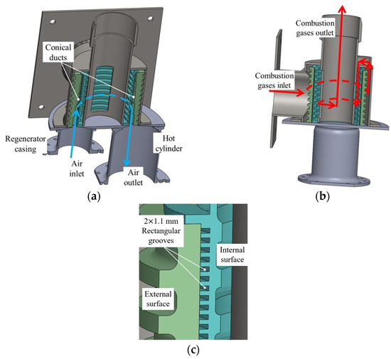
Figure 1.
Experimental Stirling heater: (a) working gas circulation inside; (b) combustion gas circulation; (c) details of inner grooves and outer fins.
As can be seen in Figure 1b, combustion gases reach the heater from the boiler and surround the outer surface of the heater, to subsequently access the interior of the heater and travel the interior surface in the opposite direction. Finally, the combustion gases are introduced inside an outlet duct to be evacuated from the exchanger. Both outer and interior surfaces are provided with 4 mm-width annular fins spaced 6 mm, avoiding narrow gaps and therefore having fewer fouling problems than the equivalent bundle of tubes.
This experimental heater was coupled to a 30 kW VETO biomass boiler for characterisation tests. The boiler’s manufacturer was required to have a bypass installed in the boiler enclosure capable of directing a flow of combustion gases towards the heater of a Stirling engine with regulation possibilities.
In the initial arrangement, the combustion gases were extracted from the boiler by means of an electrical fan, forcing them to flow around the Stirling heater, and then supplied back to the boiler, as shown in Figure 2.
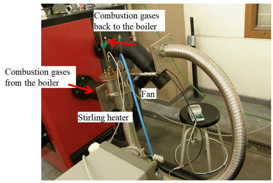
Figure 2.
Initial arrangement of the connection between the boiler and heater.
With this configuration, the exhaust gas temperature around the Stirling heater ranged between 200 °C and 250 °C, with combustion chamber temperatures of about 500 °C, values that were considered low for both variables. In the same conditions, the heater wall temperature reached 150 °C, far from the 400–600 °C interval usually considered necessary for the operation of medium- to high-temperature differential Stirling engines.
Wood pellets with the composition and highest heating value (HHV) shown in Table 1 were supplied to the boiler by means of an endless screw, which, in the default setpoint, worked 0.5 s in each 40 s interval. To increase the temperature levels, the first modification adopted was to change the pellet flow rate, changing the working cycle of the feeding endless screw. After many tests, it was found that the maximum combustion chamber temperature, in the range from 700 to 750 °C, was obtained with a feeding rate of 1 s in each 20 s interval, corresponding to a pellet flow rate of 0.3 kg/min.

Table 1.
Characteristics of the pellets used in the tests [27].
The second parameter analysed to increase the temperature level was the mass flow rate of combustion gases through the heater. As the presence of the heater itself means an important pressure drop in the exhaust gases, it is necessary to force them with a fan, but the flow rate of the gases was insufficient even with the fan operating at maximum power. For this reason, the arrangement of the ducts was modified, so that the combustion gases are not returned to the boiler after circulating through the Stirling heater but rather sent directly to the chimney to reduce pressure losses.
Figure 3 shows the final arrangement, where the connecting duct between the boiler and the inlet to the Stirling heater was removed to avoid heat losses and to provide an additional reduction in the pressure drop. The reduction in the distance between the burner and the Stirling heater is very influential on the gas temperature around the heater, and variations of only 5 cm that could lead to temperature variations of 100 °C have been reported [28]. Finally, the Stirling heater was covered with thermal insulation, and with these modifications, the exhaust gas temperature around the heater ranged between 450 and 470 °C, with the heater wall temperature close to 400 °C, which was considered acceptable to carry out the experimental tests.
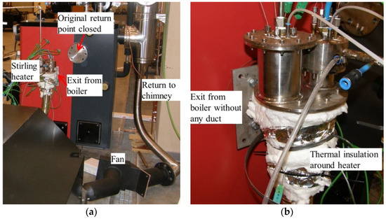
Figure 3.
Final arrangement of experimental apparatus: (a) general overview; (b) details of connection between the heater and boiler.
These initial preparations made it possible to prove that the optimal connection between a Stirling engine and a biomass boiler is in itself a research topic that not only affects the operating conditions of the engine but also affects the control strategies of the boiler. For example, the modifications adopted may have an influence on the control of the boiler, since the exhaust gases sent to the Stirling heater are returned directly to the chimney, and therefore the temperature at the connection between the boiler and the chimney could be lower than expected for conventional heating applications. This would be interpreted by the boiler control as a misfunction and ignition fail, so the ignition routine would be restarted again. After three ignition attempts, the boiler control would stop the operation for safety reasons. In addition, the varying amounts of heat sent from the boiler to the engine can determine the shutdown of the boiler burner when the maximum boiler hot water setpoint temperature is reached, and consequently the indirect shutdown of the engine. In short, control strategies must consider both boiler and engine operations, which considerably increases the number of control variables.
2.2. Variables Influencing Friction and Convective Heat Transfer
The frictional pressure losses in the heater depend on the characteristic parameters of the geometry, the physical properties of the working gas and the operating conditions. Therefore, assuming a one-dimensional flow model, and using nomenclature similar to that commonly used for Stirling engines, for ease of comparison, the local and instantaneous pressure gradient can be expressed by the following functional relationship [18]:
where is the hydraulic radius, and , , and are, respectively, the density, viscosity, pressure and velocity of the working gas.
By integrating over the heater length , the total instantaneous pressure drop is obtained. This procedure allows the gas flow to be characterised by a spatially averaged instantaneous velocity, i.e., , where is the mass flow rate and is the heater cross-sectional area. The list of influencing variables is completed with the boundary conditions, i.e., the wall temperature , the average gas temperature and the gas temperature difference , where and are the gas temperatures at the inlet and outlet sections of the heater. To generalise the geometry, the local hydraulic radius can be replaced by the hydraulic radius characteristic of the heater as a whole, defined as , where and are, respectively, the dead volume and the wetted area of the heater. Thus, the following expression can be written [18]:
If , , and are used as reference quantities, this expression leads to an equivalent functional relationship between six dimensionless groups, namely [18]:
where is the coefficient of friction, is the Reynolds number and is the Mach number, assuming that the working gas behaves as an ideal gas at temperature and that is its specific gas constant.
Using a similar procedure, the convective heat transfer coefficient can be expressed by the following functional relationship [18]:
where the characteristic properties of the thermal behaviour of the gas, namely, its specific heat capacities at constant pressure and volume, and , and its thermal conductivity , have been included. However, the pressure has not been explicitly included, since the temperature range is considered and is determined by and .
If , , , and are used as reference quantities, this expression leads to an equivalent functional relationship between eight dimensionless groups, namely [18]:
where is the Stanton number, is the Prandtl number and is the adiabatic gas coefficient.
Expressions (3) and (5) can be simplified by taking into account that negligible compressibility effects were estimated from analyses performed in previous works, for the typical operating range of an experimental micro-CHP unit based on a solar Stirling engine [18]. Consequently, the characterisation of the heater designed for biomass applications was performed neglecting the influence of , i.e., using the following functional relationships:
2.3. Instrumentation and Data Acquisition Features
The pressure at the inlet section of the heater was measured with a pressure transducer, while the pressure drop along the heater was measured with a water column differential manometer. The flow rate of air circulating inside the heater was measured and controlled by means of a mass flow regulator. Temperatures were measured by means of type K thermocouples, and all the sensors were connected to an Agilent 34970A data logger with an Agilent 34901A data acquisition board. This data logger was connected to a PC with LabView and MatLab scripts for data acquisition and post-processing.
For every test condition, 10 measurements were taken during a 10 s period, checking stability and steady conditions. The mean value of those 10 measurements was assumed to be the representative test value for each variable.
Table 2 shows the main specifications of the sensors used, whose arrangement in the experimental installation can be seen in Figure 4.
Table 2.
Specifications of sensors used for the heater characterisation.
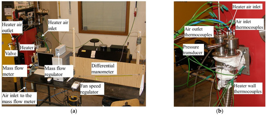
Figure 4.
(a) Overview of sensors and ancillary equipment. (b) Details of heater connections.
3. Results
3.1. Experimental Characterisation of Pressure Losses and Convective Heat Transfer
The heater was tested at four temperature levels, with different flow rates and inlet pressures for each temperature, providing 157 experimental conditions. Among these 157 analysed conditions, inconsistent results were obtained only for 19 cases, which were rejected from the analysis.
For the coefficient of friction, the following correlation was obtained, which fits the experimental measurements in the ranges , and , with values of and RMSE = 5.0%:
For the Stanton number, the following correlation was obtained, which fits the experimental measurements, in the validity ranges mentioned above, with values of and RMSE = 6.5%:
The agreement between the experimental measurements and correlation predictions can be seen in Figure 5 and Figure 6, where the dashed lines represent the ±10% relative error limits.
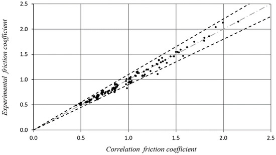
Figure 5.
Comparison between experimental and correlation values of the friction coefficient.
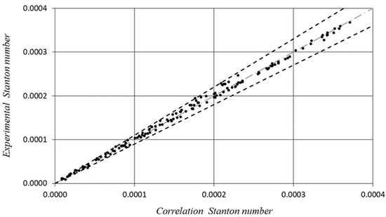
Figure 6.
Comparison between experimental and correlation values of the Stanton number.
The characterisation tests also made it possible to obtain a first impression of the fouling created on the walls of the heater by the combustion of biomass. Figure 7 shows that no significant signs of fouling were evidenced after 68 h of operation. This observation agrees with Palsson and Carlsen’s statement [29], as flame temperatures in the experiments are probably below the ash melting point. In any case, this preliminary observation will have to be corroborated by further experiments selecting different types of biomass and using longer operation periods.
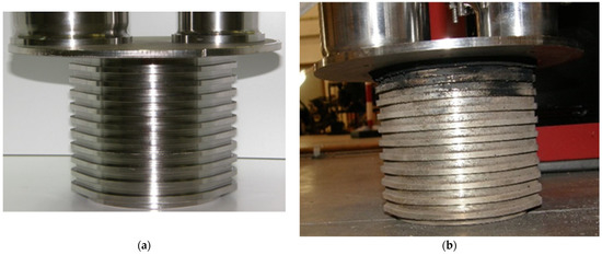
Figure 7.
External surface of Stirling heater (a) before characterisation tests and (b) after 68 h of operation with wood pellets.
3.2. CFD Model of the Heater Performance
Due to limitations in the experimental apparatus, the correlations do not cover the full range of engine operation, so a CFD model was developed to estimate the heater performance for experimental conditions not considered in the characterisation tests. In addition, the numerical simulation can provide information about the distribution of temperature and mass flow in the different slots, which are parameters as difficult to measure as they are relevant for heater analysis.
The CFD model was created using the commercial CFD software ANSYS 16. This code allows for simultaneously analysing problems of heat transfer and fluid dynamics by solving the Navier–Stokes equations, including the energy equation, through the finite volume method.
3.2.1. Computational Field and Boundary Conditions
The discretised 3D geometry was generated using the software GAMBIT, while the numerical simulations were realised by means of the software FLUENT 16.2. The symmetry of the geometry allowed the calculation of only half of the heater, as shown in Figure 8a. The domain was discretised with an unstructured mesh formed by prism and tetrahedral cells. Figure 8b shows how the mesh was refined at regions with potentially higher field gradients, near the grooves and at the air inlet and outlet sections. The solid materials making up the walls of the heater were meshed to analyse the effects of heat conduction. Since a previous study found that the variation in results was negligible with mesh sizes of more than 1 million cells [19], in this case, the computations were performed with a mesh of approximately 4,200,000 cells, which was considered sufficient to obtain the behaviour of the air near the grooves in detail.
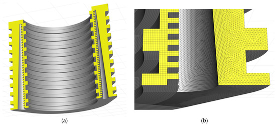
Figure 8.
(a) Half of the grooved heater as modelled in CFD simulations. (b) Detail of the mesh in the grooved area of the heater.
As for the models, the RNG model was selected to take into account the turbulence effects in the fluid flow, including buoyancy effects. This decision was taken because this type of model led to satisfactory results with turbulent flows and heat transfer for similar cases [30], and after checking that, for this geometry and meshing, the RNG and SST turbulence models lead to results with differences of less than 0.9%, but also to ensure that the comparison with the cylindrical rod heater is based on the same type of model. On the other hand, it was assumed that the working gas behaves like an ideal gas, and the solid material conforming to the experimental heater is a metal alloy of Inconel 625, with a density of 8440 kg/m3, specific heat of 410 J/(kg·K) and thermal conductivity of 9.8 W/(m·K).
For the boundary conditions, illustrated in Figure 9, it was assumed that the heat transfer through the outer walls of the heater, which are in contact with the combustion gases, is essentially by convection. On the other hand, the upper and lower surfaces of the heater were considered adiabatic, as the experimental unit was thermally insulated. Regarding the air inlet and outlet, the simulations were carried out assuming that the air enters the heater at the ambient temperature of 293 K, while the outlet air temperature is one of the numerical results obtained. The conditions of the mass flow rate and inlet air pressure were varied from experiment to experiment, while a constant value of the pressure was assumed at the heater outlet.
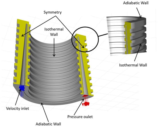
Figure 9.
Boundary conditions assumed in the CFD modelling.
Finally, in order to make the calculations accurate, a second-order discretisation was adopted, with the convergence criterion being that the value of the normalised residuals should be less than 10−5.
Ten experimental points were selected among the 157 available, to be compared with the CFD model simulations. Figure 10 summarises the result of the comparison, using the linear regression method with a trend line forced through the origin. Although some discrepancy between the model predictions and experimentation is observed at some points, the numerical simulations are considered to follow the same trend as the experiments, as the regression fit between both sets of values results in a trend line similar to the identity line and with an acceptable coefficient of determination.
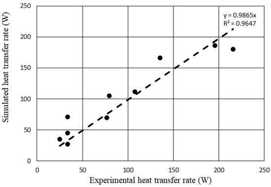
Figure 10.
Correlation between simulation and experimental results for the rectangular-grooved heater.
3.2.2. CFD Simulation Results for Selected Operating Conditions
The CFD model allows the behaviour of the heater to be studied under operating conditions different from those tested experimentally. Table 3 shows the conditions considered in 10 simulation cases, which are consistent with the nominal engine operating conditions mentioned above, namely, bar, and rpm. In all the simulations, the temperature at the external surface of the heater, , was supposed to be at 750 °C, which seems a reasonable value to guarantee values over 600–700 °C at the inner surface, in contact with the working gas. An air inlet temperature of was also assumed, as in engine operation, air enters the heater from the regenerator. The table shows the corresponding mass flow rate values and the main results of the simulations, i.e., air temperature at the exit section, ; average heater wall temperature in contact with the working gas, ; pressure drop along the heater, ; and heat transfer rate, .
Table 3.
Simulation conditions and CFD results.
On the other hand, the temperature distribution over the wall in contact with the gas circuit is an interesting topic that cannot be measured but is obtained by CFD modelling. Figure 11 shows the temperature distribution in the axial mid-plane of the heater’s rectangular grooves for simulation case No.3. It can be observed that the wall temperature decreases in the areas in contact with the gas circuit, but no hot spots are generated, so the temperature distribution simulation seems acceptable.
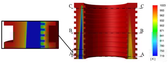
Figure 11.
Temperature distribution at heater mid-plane for simulation case No.3 and situation of sections A–C.
As for the temperature of the working gas, it clearly increases from the gas inlet in the bottom left of Figure 10 to the outlet in the bottom right. Figure 12 shows the temperature distributions in three sections of different heights, marked in Figure 11. The wall temperature varies in section AA, as this is the inlet/outlet section of the heater, while in sections BB and CC, the wall temperature does not vary significantly. The gas reaches wall temperature in most of the CC section, which is probably due to the low mass flow rates in the grooves near the CC section. The gas temperature at the outlet of the heater is lower than in the CC section, because the gas coming from this section is mixed in the exit manifold with lower-temperature gas flowing through grooves in sections closer to the outlet.
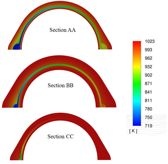
Figure 12.
Temperature distribution at three sections of Figure 10 in simulation case No.3.
Figure 13 and Figure 14 show, respectively, the pressure variation and gas velocity distribution for the same simulation case, assuming that the reference pressure is at the outlet section of the heater. Both figures confirm that there is hardly any gas flow through the grooves furthest away from the inlet and outlet sections of the heater, suggesting that the design of this area should be reviewed in future optimisations.
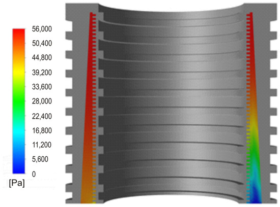
Figure 13.
Pressure distribution at heater mid-plane in simulation case No.3.
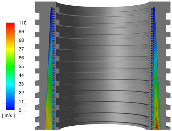
Figure 14.
Velocity distribution at heater mid-plane in simulation case No.3.
4. Discussion
A main characteristic of a Stirling engine is the rate of heat transfer that the heater must supply to the gas circuit in order to develop a given indicated power with efficiency , i.e., the quotient .
The indicated power depends on more than twenty parameters, including geometrical characteristics of the gas circuit and drive mechanism, working gas and regenerator material properties, mean pressure, heater and cooler wall temperatures, and operating speed [24,25]. From thermodynamic concepts and experimental results of benchmark engines, it has been deduced that the indicated power developed by a Stirling engine under actual operating conditions satisfies the following equation [26]:
where , , is the characteristic Mach number, which can be interpreted as the dimensionless engine speed, is the swept volume of the engine, is the indicated work per cycle under quasi-static conditions and is the cooler wall temperature. On the other hand, and designate, respectively, coefficients of indicated power losses caused by irreversibilities. Engines with the same temperature and swept and dead volume ratios would have the same value but different and values, due to the use of different working gases, mean pressures or heat exchanger geometries, which would, in turn, lead to different losses inside heat exchangers. The coefficients and depend on engine geometrical parameters, working gas and regenerator material properties, the ratio between cooler and heater wall temperatures, , and the characteristic pressure number , where is the working gas viscosity. However, they do not depend on .
Under ideal conditions, the indicated efficiency of a Stirling cycle would be equal to the efficiency of a reversible Carnot cycle, i.e., . However, under real conditions, the efficiency is lower, both because the actual indicated work is less than the maximum theoretically achievable, i.e., , and because the heat supplied by the heater in each cycle is greater than that corresponding to ideal conditions, i.e., .
Therefore, due to the thermo-mechanical irreversibilities inherent in actual operation, the heater must provide the following heat transfer rate increase:
To facilitate comparisons, Equation (11) can be generalised by using dimensionless variables, so that it can be written as
The heat transfer rate increase caused by irreversibilities is an under-researched feature of Stirling heaters. In the only known previous analyses of this issue [3,19], it has been found that is related to characteristic variables of the gas circuit performance that might intuitively be considered non-influential in external combustion engines.
In the case of the SOLO V160 engine tube heater, the following correlation was obtained [3]:
In the case of the cylindrical rod heater designed for solar energy conversion, the following correlation was obtained [18,19]:
Equations (13) and (14) are examples of the relationship between the heat transfer rate and characteristic parameters of the thermodynamic circuit. The use of dimensionless variables facilitates the comparison between prototypes.
The results of the CFD model allow a comparative analysis of the non-tubular biomass heater. For this purpose, the CFD results listed in Table 3 were converted into the corresponding dimensionless values, as shown in Table 4.
Table 4.
Dimensionless values corresponding to simulation cases.
These data fit the following equation, with RMSE = 0.65% and R2 = 0.9999:
Figure 15 facilitates the comparison between values of calculated using Equations (13)–(15). The red lines correspond approximately to nominal mean pressure conditions. Note that the ratio between the average pressure of 125 bar for the V160 engine heater and the value of 6.9 bar for the non-tubular heaters is equal to 18.1, while the ratio between the corresponding values of and is approximately equal to 6.2, due to differences in geometry, operation temperatures and working gas. To assess the influence of on the respective correlations, this figure also shows black lines for the values , which corresponds to low mean pressure levels in the non-tubular heaters, and , which corresponds to approximately half of the minimum operating pressure of the V160 engine.
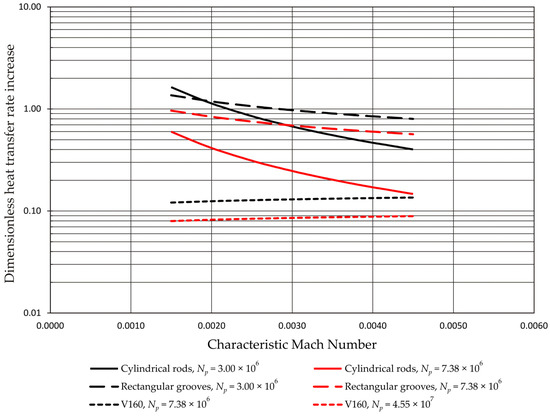
Figure 15.
Comparison between correlations of heat transfer rate increase due to irreversibilities.
The differences observed in Figure 15 are due not only to the different values of but also to the different degrees of development of designs pending optimisation and of a design that has been improved over several decades. As expected, the V160 engine heater, using helium as the working gas, has the lowest values of , but it is interesting to note that the cylindrical rod heater, using air as the working gas, would have not very different values at equal , for values greater than , which are not very far from the nominal conditions.
The numerical results of simulation case No.4, which is representative of the rated conditions, provide a comparative evaluation of the engine performance with both non-tubular heaters. Under these conditions, using numerical simulations and correlations of indicated power and engine speed based on experimental data from benchmark engines [31], a maximum indicated power of the order of 700 W at 900 rpm was predicted for the unit with the cylindrical rod heater [18]. Using an analogous procedure, as the grooved heater has a smaller dead volume and a larger heat exchange surface than the cylindrical rod heater, values of , mm, and are obtained for the grooved heater, leading to a maximum indicated power of 815 W at 900 rpm and an indicated efficiency of 20%. As Figure 15 shows, the increase in the heat transfer rate due to irreversibilities in the grooved heater is almost three times higher than the value obtained with the cylindrical rod heater. However, an increase in the indicated efficiency can be expected if the stagnant flow areas predicted by the CFD model are avoided through future geometric optimisation.
5. Conclusions
The connection between the heater of a Stirling engine and a commercial biomass boiler is not a trivial task, as it determines the operating temperatures that can be reached, not only because of geometrical issues but also because a non-specifically designed control system can lead to undesired shutdowns.
Experimental correlations for heat transfer and pressure drop were obtained for a new non-tubular heater design, intended to be adapted to a prototype biomass-driven micro-CHP unit. No major fouling problems were observed during the characterisation tests.
The CFD model developed for the new heater made it possible to estimate the operating performance under conditions different from those tested during the experimental characterisation, and to analyse operating parameters that are practically impossible to measure.
The temperature distribution on the heater wall appears to be adequate. However, areas of stagnant flow were detected, suggesting the possibility of improving the heat exchanger performance through detailed geometrical modifications.
The CFD model predictions allowed comparisons to be made with the heat transfer rate achieved with two other heaters with different geometries. The tube bundle heater of the SOLO V160 engine shows the best comparison results and is recommended for applications based on convective heat transfer with flue gases that do not cause fouling problems. With respect to the cylindrical rod heater, previously designed for a solar micro-CHP unit, the dimensionless heat transfer rate increase due to irreversibilities approaches the values of the V160 engine heater when the characteristic dimensionless numbers of pressure and velocity are close. For the grooved heater designed for biomass applications, the dimensionless increase in the heat transfer rate due to irreversibilities is almost three times the value obtained with the cylindrical rod heater. However, the grooved heater has a smaller dead volume and a larger heat exchange surface, so it is estimated that the engine would develop a maximum indicated power of 815 W at 900 rpm, which is higher than that obtained with the cylindrical rod heater. The corresponding indicated efficiency, 20%, would be lower but can be improved by geometric modifications to avoid the areas of stagnant flow observed in the CFD simulations.
Author Contributions
Conceptualisation, methodology, investigation and resources, J.-I.P. and D.G.; software, validation and formal analysis, M.-J.S., D.G. and E.B.; data curation and writing—original draft preparation, D.G. and M.-J.S.; writing—review and editing, J.-I.P. and D.G.; supervision, project administration and funding acquisition, J.-I.P. All authors have read and agreed to the published version of the manuscript.
Funding
This research was co-financed by the European Union, through the FEDER Funds, and the Principality of Asturias, through the Science, Technology and Innovation Plan 2013–2017, grant number GRUPIN–095–2013. The APC is excluded from funding.
Institutional Review Board Statement
Not applicable.
Informed Consent Statement
Not applicable.
Data Availability Statement
Not applicable.
Conflicts of Interest
The authors declare no conflict of interest.
References
- Sustainable Development Goals. Available online: https://www.un.org/sustainabledevelopment/energy (accessed on 10 October 2022).
- Babaelahi, M.; Sayyaadi, H. A new thermal model based on polytropic numerical simulation of Stirling engines. Appl. Energy 2015, 141, 143–159. [Google Scholar] [CrossRef]
- García, D.; González, M.A.; Prieto, J.-I.; Herrero, S.; López, S.; Mesonero, I.; Villasante, C. Characterisation of the power and efficiency of Stirling engine subsystems. Appl. Energy 2014, 121, 51–63. [Google Scholar] [CrossRef]
- Breeze, P. Piston Engine-Based Power Plants; Academic Press: London, UK, 2018. [Google Scholar] [CrossRef]
- Zhu, S.; Yu, G.; Liang, K.; Dai, W.; Luo, E. A review of Stirling-engine-based combined heat and power technology. Appl. Energy 2021, 294, 116965. [Google Scholar] [CrossRef]
- Ferreira, A.C.; Silva, J.; Teixeira, S.; Teixeira, J.C.; Nebra, S.A. Assessment of the Stirling engine performance comparing two renewable energy sources: Solar energy and biomass. Renew. Energy 2020, 154, 581–597. [Google Scholar] [CrossRef]
- Hargreaves, C.M. The Philips Stirling Engine; Elsevier: Amsterdam, The Netherlands, 1991. [Google Scholar]
- Baumüller, A.; Lundholm, G.; Lundsröm, L.; Schiel, W. Development history of the V160 and SOLO Stirling 161 engines. In Proceedings of the 9th International Stirling Engine Conference, Pilanesburg, South Africa, 2–4 June 1999; pp. 23–32. [Google Scholar]
- Mahkamov, K.; Trukhov, V.S.; Lejebokov, A.; Tursunbaev, I.A.; Orunov, B.; Korobkov, A.; Ingham, D.B. Development of Stirling engines for energetic units. In Proceedings of the 9th International Stirling Engine Conference, Pilanesburg, South Africa, 2–4 June 1999; pp. 1–7. [Google Scholar]
- Yang, H.-S.; Ali, M.A.; Teja, K.V.R.; Yen, Y.-F. Parametric study and design optimization of a kW-class beta-type Stirling engine. Appl. Therm. Eng. 2022, 215, 119010. [Google Scholar] [CrossRef]
- Kuosa, M.; Kaikko, J.; Koskelainen, L. The impact of heat exchanger fouling on the optimum operation and maintenance of the Stirling engine. Appl. Therm. Eng. 2007, 27, 1671–1676. [Google Scholar] [CrossRef]
- Schneider, T.; Müller, D.; Karl, J. A review of thermochemical biomass conversion combined with Stirling engines for the small-scale cogeneration of heat and power. Renew. Sustain. Energy Rev. 2020, 134, 110288. [Google Scholar] [CrossRef]
- Godett, T.M.; Meijer, R.J.; Verhey, R.P.; Pearson, C.J.; Khalili, K. STM4-120 Stirling Engine Test Development; SAE Technical Paper 890149; Society of Automotive Engineers: Warrendale, PA, USA, 1989. [Google Scholar] [CrossRef]
- Hoshino, T.; Naito, H.; Fujihara, T.; Eguchi, K. NAL research program on space solar power technology-NALSEM500 Stirling alternator and solar receiver. In Proceedings of the 9th International Stirling Engine Conference, Pilanesburg, South Africa, 2–4 June 1999; pp. 233–238. [Google Scholar]
- Kaliakatsos, D.; Cucumo, M.; Ferraro, V.; Mele, M.; Cucumo, S.; Miele, A. Performance of Dish-Stirling CSP system with dislocated engine. Int. J. Energy Environ. Eng. 2017, 8, 65–80. [Google Scholar] [CrossRef]
- Rahman, N.K.M.N.A.; Saadon, S.; Man, M.H.C. Waste Heat Recovery of Biomass Based Industrial Boilers by Using Stirling Engine. J. Adv. Res. Fluid Mech. Thermal Sci. 2022, 89, 1–12. [Google Scholar] [CrossRef]
- Gomaa, A.; Alsit, A.; Dol, S.S. Heat Transfer Enhancement in Stirling Engines Using Fins with Different Configurations and Air Flow. CFD Lett. 2022, 14, 16–31. [Google Scholar] [CrossRef]
- García, D.; Prieto, J.-I. A non-tubular Stirling engine heater for a micro solar power unit. Renew. Energy 2012, 46, 127–136. [Google Scholar] [CrossRef]
- García, D.; Suárez, M.-J.; Blanco, E.; Prieto, J.-I. Experimental correlations and CFD model of a non-tubular heater for a Stirling solar engine micro-cogeneration unit. Appl. Therm. Eng. 2019, 153, 715–725. [Google Scholar] [CrossRef]
- Afzal, A.; Mohammed Samee, A.D.; Javad, A.; Shafvan, S.A.; Ajinas, P.V.; Ahammedul Kabeer, K.M. Heat transfer analysis of plain and dimpled tubes with different spacings. Heat Transf.—Asian Res. 2018, 47, 556–568. [Google Scholar] [CrossRef]
- Soudagar, M.E.M.; Kalam, M.A.; Sajid, M.U.; Afzal, A.; Banapurmath, N.R.; Akram, N.; Mane, S.; Saleel, C.A. Thermal analyses of minichannels and use of mathematical and numerical models. Numer. Heat Transf. Part A Appl. 2020, 77, 497–537. [Google Scholar] [CrossRef]
- Kumar, R.; Cuce, E.; Kumar, S.; Thapa, S.; Gupta, P.; Goel, B.; Saleel, C.A.; Shaik, S. Assessment of the Thermo-Hydraulic Efficiency of an Indoor-Designed Jet Impingement Solar Thermal Collector Roughened with Single Discrete Arc-Shaped Ribs. Sustainability 2022, 14, 3527. [Google Scholar] [CrossRef]
- Finkelstein, T. Generalized thermodynamic analysis of Stirling engines. In Proceedings of the SAE Winter Annual Meeting, Detroit, MI, USA, 1960. paper 118B. [Google Scholar]
- Organ, A.J. The Regenerator and the Stirling Engine; Mechanical Engineering Publications: London, UK, 1997. [Google Scholar]
- Organ, A. Thermodynamics and Gas Dynamics of the Stirling Cycle Machine; Cambridge University Press: Cambridge, UK, 1992. [Google Scholar]
- Prieto, J.-I.; Gonzalez, M.A.; Gonzalez, C.; Fano, J. A new equation representing the performance of kinematic Stirling engines. Proc. Inst. Mech. Eng. Part C J. Mech. Eng. Sci. 2000, 214, 449–464. [Google Scholar] [CrossRef]
- García, R.; Pizarro, C.; Álvarez, A.; Lavín, A.G.; Bueno, J.L. Study of biomass combustion wastes. Fuel 2015, 148, 152–159. [Google Scholar] [CrossRef]
- Cardozo, E.; Erlich, C.; Malmquist, A.; Alejo, L. Integration of a wood pellet burner and a Stirling engine to produce residential heat and power. Appl. Therm. Eng. 2014, 73, 671–680. [Google Scholar] [CrossRef]
- Palsson, M.; Carlsen, H. Development of a wood powder fuelled 35 kW Stirling CHP unit. In Proceedings of the 11th International Stirling Engine Conference, Rome, Italy, 19–21 November 2003; pp. 221–230. [Google Scholar]
- Launder, B.E.; Spalding, D.B. The numerical computation of turbulent flows. Comput. Methods Appl. Mech. Eng. 1974, 3, 269–289. [Google Scholar] [CrossRef]
- Sala, F.; Invernizzi, C.-M.; García, D.; González, M.-A.; Prieto, J.-I. Preliminary design criteria of Stirling engines taking into account real gas effects. Appl. Therm. Eng. 2015, 89, 978–989. [Google Scholar] [CrossRef]
Publisher’s Note: MDPI stays neutral with regard to jurisdictional claims in published maps and institutional affiliations. |
© 2022 by the authors. Licensee MDPI, Basel, Switzerland. This article is an open access article distributed under the terms and conditions of the Creative Commons Attribution (CC BY) license (https://creativecommons.org/licenses/by/4.0/).