Article

Group-Sparse Feature Extraction via Ensemble Generalized Minimax-Concave Penalty for Wind-Turbine-Fault Diagnosis

1
School of Aerospace Science and Technology, Xidian University, Xi’an 710071, China
2
School of Guangzhou Institute of Technology, Xidian University, Guangzhou 510555, China
3
School of Aerospace Engineering, Xiamen University, Xiamen 361005, China
*
Author to whom correspondence should be addressed.
Sustainability 2022, 14(24), 16793; https://doi.org/10.3390/su142416793
Submission received: 25 October 2022 / Revised: 11 December 2022 / Accepted: 12 December 2022 / Published: 14 December 2022
(This article belongs to the Special Issue Applied Artificial Intelligence for Sustainability)

Abstract

:
Extracting weak fault features from noisy measured signals is critical for the diagnosis of wind turbine faults. In this paper, a novel group-sparse feature extraction method via an ensemble generalized minimax-concave (GMC) penalty is proposed for machinery health monitoring. Specifically, the proposed method tackles the problem of formulating large useful magnitude values as isolated features in the original GMC-based sparse feature extraction method. To accurately estimate group-sparse fault features, the proposed method formulates an effective unconstrained optimization problem wherein the group-sparse structure is incorporated into non-convex regularization. Moreover, the convex condition is proved to maintain the convexity of the whole formulated cost function. In addition, the setting criteria of the regularization parameter are investigated. A simulated signal is presented to verify the performance of the proposed method for group-sparse feature extraction. Finally, the effectiveness of the proposed group-sparse feature extraction method is further validated by experimental fault diagnosis cases.

1. Introduction

As one of the most common types of mechanical equipment, the wind turbine has played an important role in industrial applications. It is of great significance to detect the various faults of wind turbine as early as possible to prevent economic losses and casualties [1]. Extracting the periodic impact signal hidden in measured noisy vibration signals has been a focus in the field of signal processing because of its vital importance in the vibration-based condition monitoring and fault detection of wind turbines [2]. For instance, rolling bearings are components that are widely used in rotating machinery. Inner and outer ring failures caused by the abnormal operation of bearings have become one of the most common causes of wind turbine failures [3]. However, the observed vibration signals are often submerged in very serious background noise, which poses a challenge to the extraction of transient signals [4,5]. Therefore, whether the transient impulse submerged in the strong background noise can be successfully detected is key to extracting fault information.
Numerous diagnostic techniques have been proposed, and some of them use different transforms to extract features, such as short-time Fourier transform (STFT) [6,7] and wavelet transform [8,9,10]. Some methods adopt the idea of signal decomposition, such as empirical mode decomposition (EMD) [11,12], variational mode decomposition (VMD) [13,14,15], local mean decomposition [16], the stochastic resonance technique [17,18] and blind deconvolution algorithms [19]. There are also some methods that combine traditional time-frequency analysis with other techniques suitable for transient detection, such as the method based on spectral kurtosis (SK) [20,21] and so on. Machinery fault classification is also a popular research topic in this area, which is based on machine learning. Most of these methods improve diagnostic performance by applying statistical methods to collected vibration signals. Among these methods, support vector machines and algorithms based on the BP neural network have achieved remarkable results in mechanical fault diagnoses [22].
In recent years, researchers from the field of signal processing have paid more attention to sparse representation. The purpose of applying sparse representation is to extract correlated information in the signal. The well-known basis pursuit method solves the sparse optimization problem by using the 𝓁 1 norm [23], which is a typical convex-optimization problem. It can converge to the global optimal solution of the objective function using the split-variable-augmented Lagrangian shrinkage algorithm (SALSA) [24]. However, the application of 𝓁 1 norm regularization underestimates the magnitude component to be solved. Therefore, optimization problems based on non-convex regularization terms have attracted the attention of many scholars. The advantage of adopting non-convex regularization is that it can estimate the high-amplitude components of the signal more accurately. However, the application of non-convex regularization inevitably weakens the strict convexity of the objective function [25]. In response to this problem, some scholars have turned their attention to convex optimization via non-convex regularization. The degree of non-convexity of non-convex regularization can be adjusted by changing the controllable parameters [26]. In this way, the objective function could converge to the global minimum under the condition that the whole objective function is convex.
It is worth nothing that when large-amplitude coefficients form groups (clusters), the 𝓁 1 norm and other separable sparsity models do not capture the tendency of the coefficients to group (group sparsity) [27]. A large number of scholars have made efforts in the estimation and reconstruction of group-sparse signals. In the case of group overlap, an algorithm called overlapping group shrinkage (OGS) is presented, which is dedicated to seeking the minimization of the convex cost function [28]. Four non-convex penalty functions were proposed to enhance the extraction of sparsity, and the corresponding algorithm was given in [29]. Huang et al. constructed a multivariate variable-scale non-convex function as a regularizer in the sparse regular optimization problem [30]. By comparing with the 𝓁 1 norm, it can be observed that the non-convex penalty can estimate the high-amplitude components of the sparse solution more accurately. Fan et al. combined the tunable Q-factor wavelet transform (TQWT) with the OGS algorithm, and it showed obvious superiority in the extraction of weak magnetic signals [31]. He et al. proposed the periodicity-induced overlapping group shrinkage (POGS) technique and applied it to extract and depart the compound transient features of periodic groups [32]. Since Ivan proposed to use GMC function for sparse feature extraction, GMC function as a typical non-convex function has become the concerned of many scholars [33].
In essence, the GMC function is formed by optimizing the 𝓁 1 norm so it can achieve a sparse extraction result that is better than the 𝓁 1 norm. Based on the combination of the GMC penalty and the TQWT, He et al. proposed a novel sparsity-enhanced method and verified its reliability [34]. Liu et al. applied the GMC penalty to the recognition of impact force and showed its superiority in signal amplitude evaluation [35]. However, these recently developed diagnostic methods formulate large useful magnitude fault values as isolated features. To address this problem, a novel group-sparse feature extraction method via an ensemble generalized minimax-concave penalty is proposed in this paper for machinery health monitoring. The proposed method applies the idea of “packaging signals in the form of groups” to the GMC-regularized least-squares problem. The OGS algorithm, based on the principle of majorization–minimization (MM), is a fast iterative algorithm that can quickly converge to the optimal sparse solution of the group signal. For the feature extraction of sparse group signals using the GMC penalty, the useful fault features are modeled as group-sparse signals and are subsequently incorporated into the non-convex regularization in this paper. Moreover, the convexity condition is derived to guarantee that the objective function is still a convex-optimization problem. Finally, the forward–backward group feature extraction (FBGFE) algorithm is given to solve the formulated optimization problem. The method is applied to the analysis of simulation signals and bearing fault signals, and the processing results show that the proposed method in this paper can successfully extract fault features in strong noise. In comparison with traditional L1 norm regularization, GMC and OGS methods, the effectiveness and superiority of the proposed method are verified.
The remainder of this paper is organized as follows. In Section 2, the basic theory of the GMC penalty and the overlapping group-sparse algorithm are briefly introduced. Section 3 presents the proposed group-sparse feature extraction method via the ensemble GMC penalty for machinery health monitoring. In Section 4, the effectiveness and superiority of the proposed method is verified by numerical signals. Section 5 applies the proposed method to the fault diagnosis of rotating machinery for further validation. Finally, Section 6 summarizes the conclusion.

2. Basic Theory

2.1. GMC Penalty

The GMC penalty function can be regarded as a multivariate generalization of the minimax concave (MC) penalty function. The advantages of adopting such a penalty function are the following: (1) The strict convexity of the objective function can be ensured so that the advantages of the global minimum of convex optimization can be maintained. (2) It avoids the disadvantage of underestimating the high vibration component of traditional 𝓁 1 norm regularization and can greatly enhance the sparsity of the extracted features.
The MC function is expressed as the absolute value function subtract the one-dimensional variable-scale smooth convex Huber function. For a 0 , the expression of the Huber function is
S a ( x ) = min v i | v | + a 2 ( x v ) 2 .
Therefore, the MC function [33] is ϕ a ( x ) : , and it can be expressed as
ϕ a ( x ) = x S a ( x ) .
By extending the Huber function to the multi-dimensional case as the extended form of S a ( x ) in (1), S B ( x ) can be expressed as
S B ( x ) : = inf v R N | | v | | 1 + 1 2 | | B ( x v ) | | 2 2 .
The multivariate generalization of the MC penalty can be obtained by extending the MC function, and the GMC function [33] can be denoted as
ψ B ( x ) : = | | x | | 1 S B ( x ) .
By varying parameter B, the non-convex degree of the GMC function is tuned. As shown in Figure 1a, with the increasing of parameter a, the non-convex degree of the MC function also increases. In additional, Figure 1b shows the form of GMC with different matrix B, where the non-convex controllable parameters were set as B 1 = 0.2 0.2 0   0 0.2 0.2 , B 2 = 0.6 0.6 0   0 0.6 0.6 , B 3 = 1 1 0   0 1 1 .

2.2. Overlapping Group Shrinking Algorithm

The OGS algorithm uses a penalty function R ( x ) to minimize the cost function, which can be seen as the mixture of the 𝓁 1 norm and the 𝓁 2 norm. The expression of R ( x ) [28] is expressed as
R ( x ) = i I j J x ( i + j ) 2 1 / 2 .
For a vector x with a signal length of N, and the size of K, I and J are defined as
I = 0 , , N 1 ,
J = 0 , , K 1 .
Based on the above notation, the cost function can be defined as
F ( x ) = 1 2 | | y i , k x i , k | | 2 2 + λ R ( x i , k ) ,
where the λ is the regularization parameter. Using the MM algorithm to solve (8), the iterative solution can be obtained as
x k + 1 ( i ) = y ( i ) 1 + λ r ( i ; x ( k ) ) ,
where
r ( i ; x ( k ) ) : = j J k J x ( k ) ( i j + k ) 2 1 / 2 .
It should be noted that the OGS algorithm converges to the global optimal solution by gradually reducing the non-zero values of y to zero rather than directly reduce them to zero in any iteration. Additionally, the determination of the value of k depends on prior knowledge of the signal x.

3. The Proposed Group-Sparse Feature Extraction Method Based on Ensemble GMC

In this section, to accurately estimate group-sparse fault features, a novel group-sparse feature extraction method via the ensemble GMC penalty is proposed for machinery health monitoring. The proposed method was constructed by adopting the aforementioned penalty function as the regularization term for the optimization of least squares. Specifically, the proposed method includes the three following elements: (1) the construction of the group-sparse-enhanced optimization problem; (2) the condition that constrains the overall cost function is convex; and (3) the derived fast iterative convergence algorithm.

3.1. Optimization Problem Formulation

In order to accurately estimate group-sparse fault features from noisy signals, the following unconstrained optimization problem can be formulated.
x * = arg min x i F ( x ) = 1 2 | | y i , k x i , k | | 2 2 + λ ψ B ( x i , k ) .
Notice that in the formulated problem (11), ψ B ( x i , k ) represents the GMC penalty for the group-sparse signal x, and x * is the spare solution obtained after solving the unconstrained optimization problem.
Taking into account the group sparsity of the signal x, x i , k [28,29] in the above equation can be expressed as
x i , k = [ x ( i ) , , x ( i + k 1 ) ] i k .
Note that x i , k represents the i-th group signal with size k, and its corresponding 𝓁 1 norm is defined as
| | x i , k | | = | x ( i ) | + + | x ( i + k 1 ) | .

3.2. Convexity Condition

From the proof in section III part B in reference [29], the cost function in (11) can be written as
F ( x ) = i F i ( x i , k ) .
The expression obtained by expanding F i ( x i , k ) is
F i ( x i , k ) = 1 2 k | | y i , k x i , k | | 2 2 + λ k ( | | x i , k | | S B ( x i , k ) ) = 1 2 k | | y i , k x i , k | | 2 2 + λ k | | x i , k | | 1 1 k min v R N λ | | v i , k | | 1 + λ 2 | | B ( x i , k v i , k ) | | 2 2 = max v R N 1 2 k | | y i , k x i , k | | 2 2 + λ k | | x i , k | | 1 λ k | | v i , k | | 1 λ 2 k | | B ( x i , k v i , k ) | | 2 2 = max v R N 1 2 k x i , k T ( I λ B T B ) x i , k + λ k | | x i , k | | 1 + g ( x i , k , v i , k ) = 1 2 k x i , k T ( I λ B T B ) x i , k + λ k | | x i , k | | 1 + max v R N g ( x i , k , v i , k )   ,
where g is affine in x. The last term in (15) is convex as it is the pointwise maximum of a set of convex functions. Thus, if I λ B T B 0 or, in other words, 0 < B < I λ , then F i ( x i , k ) is a convex function. As a result, the cost function (14) can be regarded as the sum of a series of convex functions, which is also a convex function. Given the identity matrix I , matrix B can be simply specified as B = γ / λ I , which satisfies F ( x ) is convex when γ 1 . The parameter γ controls the non-convexity of the penalty ψ B . If γ = 0 , then B = 0 and the penalty is reduced to the 𝓁 1 norm. If γ = 1 , then (14) is satisfied with equality and the penalty is maximally non-convex. In practice, γ is usually recommended to be specified as a range of 0.5 γ 0.8 . It can be noted that the objective function could maintain convexity by adjusting B. Therefore, the fast iterative algorithm can converge to the global optimal solution and avoid entrapment in sub-optimal local minima.

3.3. Algorithm Implementation

To use proximal algorithms to minimize the cost function F, the optimization problem formulated in (11) can be regarded as a saddle-point problem [33], which can be written as
( x o p t , v o p t ) = arg min x R N max v R N F ( x i , k , v i , k ) .
In the above optimization problem, F ( x i , k , v i , k ) can be written as
F ( x i , k , v i , k ) = 1 2 k | | y i , k x i , k | | + λ k | | x i , k | | 1 λ k | | v i , k | | 1 + γ 2 k | | x i , k v i , k | | 2 2 .
x o p t is the obtained optimal solution with group-sparse features.
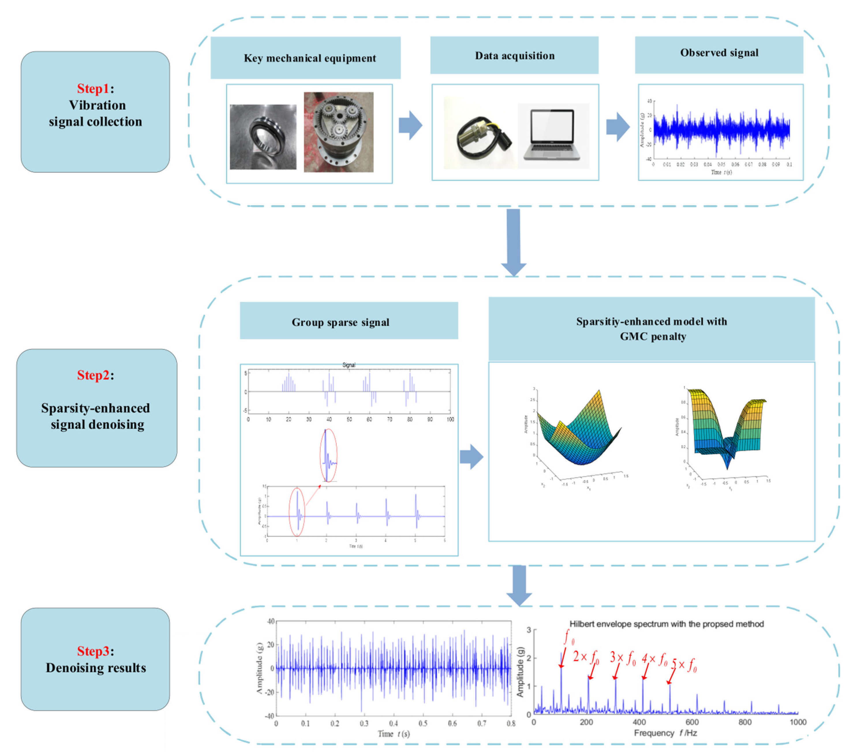
The saddle-point problem can be solved by the forward–backward (FB) algorithm. Figure 2 illustrates the procedure of the proposed group-sparse feature extraction method via the ensemble GMC penalty. Firstly, the vibration sensor is installed to collect the vibration signals through data-acquisition equipment and record the relevant parameters. Then, the collected noisy signals are processed by the proposed method to extract the corresponding fault features. Finally, the feature extraction results are shown in the time-domain form and the envelope spectrum. The FB algorithm used to extract sparse signals with group-sparse properties is defined as the forward–backward group feature extraction (FBGFE) algorithm, which is summarized in Algorithm 1. Notice that the convergence condition of the iterative algorithm proposed in this paper is that the number of iterations is reached, and the error is also controlled within the specified range. Generally, the iterated error specified is very small, e.g., 10−4.
Algorithm 1 FBGFE: Forward–backward group feature extraction algorithm
Input: y i k N , i I , k R + , λ > 0 , λ , γ , k
Initialization: ρ = max 1 , γ / ( 1 γ ) , 0 < μ < 2 / ρ
For  i = 0 , 1 , 2 ,
    w i k ( i ) = 1 k c o n v ( x i k ( i ) μ ( x i k ( i ) + γ ( v i k ( i ) x i k ( i ) ) y i k ) , h )
    v i k ( i ) = 1 k c o n v ( x i k ( i ) μ ( x i k ( i ) + γ ( v i k ( i ) x i k ( i ) ) y i k ) , h )
    x i k ( i + 1 ) = s o f t ( w i k ( i ) , μ λ )
    v i k ( i + 1 ) = s o f t ( u i k ( i ) , μ λ )
end
where i is the iteration counter.
Return: x
In order to further illustrate the formation of group sparsity, an example is given. If k = 2, then the first part in the convolution operator can be expressed as
a i k ( i ) = x i k ( i ) μ ( x i k ( i ) + γ ( v i k ( i ) x i k ( i ) ) y i k i ) = x i 0 ( i ) + x i 1 ( i ) μ ( x i 0 ( i ) + x i 1 ( i ) + γ ( v i 0 ( i ) + v i 1 ( i ) x i 0 ( i ) x i 1 ( i ) ) y i 0 i y i 1 i ) .
Note that x i 0 ( i ) + x i 1 ( i ) can be achieved by convolution, where h is an all-in-one vector with a size of 1 × K.

3.4. Remark of the Proposed Algorithm

As presented in detail in this section, the proposed group-sparse feature extraction method is closely based on GMC. The main contribution of the proposed method is that the proposed method formulates an unconstrained optimization problem wherein the group-sparse structure is incorporated into non-convex regularization, as referred to Equation (11) in Section 3.1. In other words, the original GMC-based sparse feature extraction method does not consider the promotion of features with group-sparse features. However, many prior studies have demonstrated that measured-fault vibration signals of rotating machines have group-sparse properties. Here, a signal with group-sparse properties means large magnitude signal values tend not to be isolated; instead, these large magnitude values tend to form groups [36]. To guarantee that the formulated optimization problem is strictly convex, another contribution of the proposed method is a focus on deriving the convexity condition, which is presented in detail in Section 3.2. As a result, the global minimizer can be obtained via the derived fast iterative algorithm, as described in Section 3.3.

4. Simulation Study

The objective of the present simulation experiment is to verify the validity of the proposed method and thus to better extract the sparse signal. In this section, the proposed method is compared with the OGS method, 𝓁 1 norm regularization method and GMC penalty method. The impulsive and oscillatory simulation signal is given by
y ( t ) = A × exp ( 20 t ) × sin ( 100 t ) + n s ( t )
where A is defined as the amplitude of the impulse signal, n s ( t ) is the addictive Gaussian noise, the sampling frequency is f s = 1000 Hz, the signal length is N = 6000 and the noise standard deviation is σ = 0.1 . To effectively compare the proposed method with the 𝓁 1 norm regularization, GMC penalty and OGS method, the root-mean-squared error (RMSE) and signal–noise ratio(SNR)were chosen as measures to facilitate quantitative analyses.
The calculation formula of the SNR and RMSE is defined as
S N R = 10 log 10 | | x | | 2 2 | | x x _ d e n o i s e | | 2 2
R M S E = 1 N | | x x _ d e n o i s e | | 2 2
where x represents the noise-free signal, x _ d e n o i s e stands for the denoised signal and N represents the signal length.

4.1. Simulation Validation

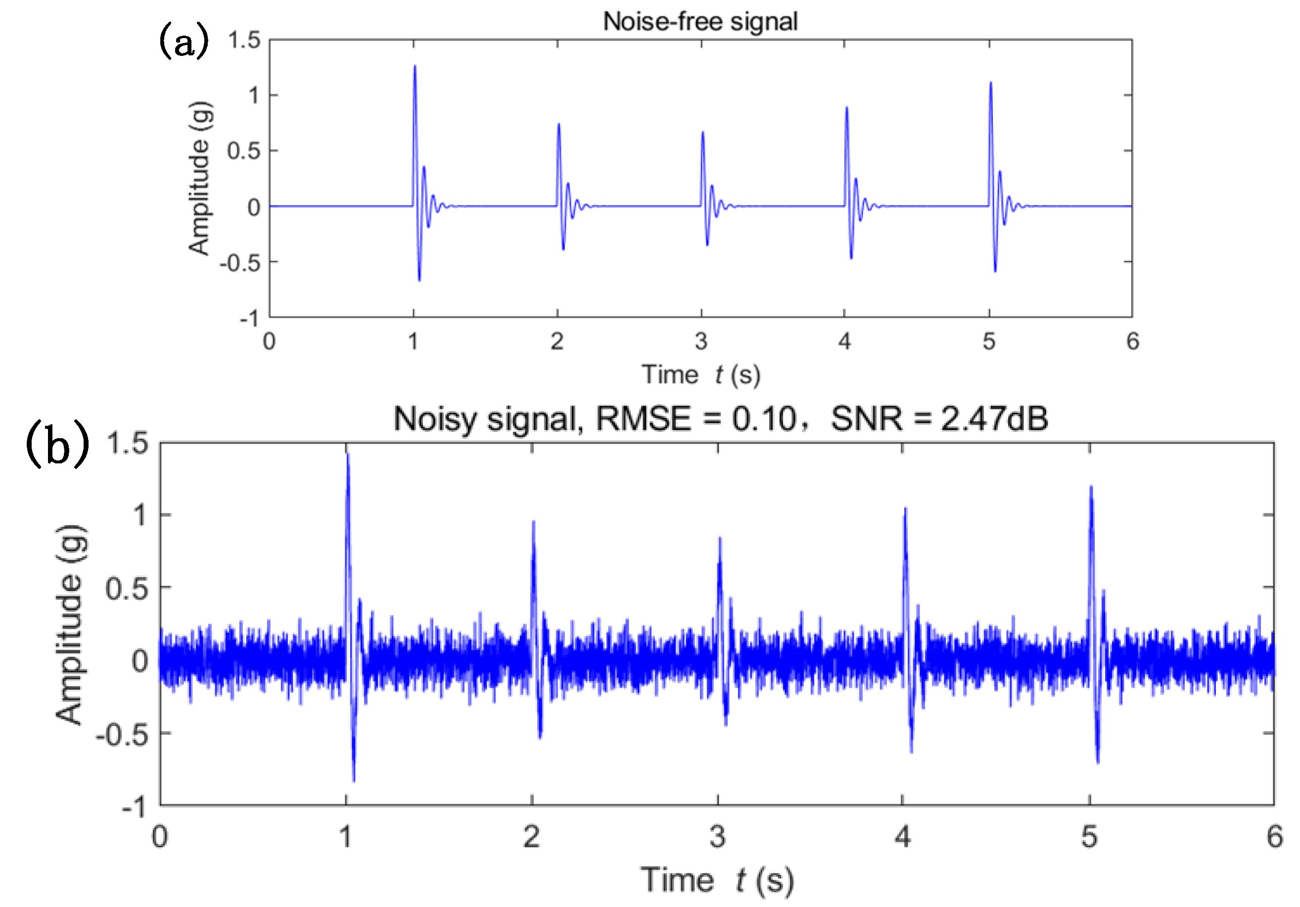
The whole simulation signal consists of five impulse signals and Gaussian noise. The simulation signal is shown in Figure 3, which is composed of the noise-free signal and the signal with Gaussian noise. The simulation noise-free signal with impulse is shown in Figure 3a. The noisy signal with Gaussian noise is shown in Figure 3b.
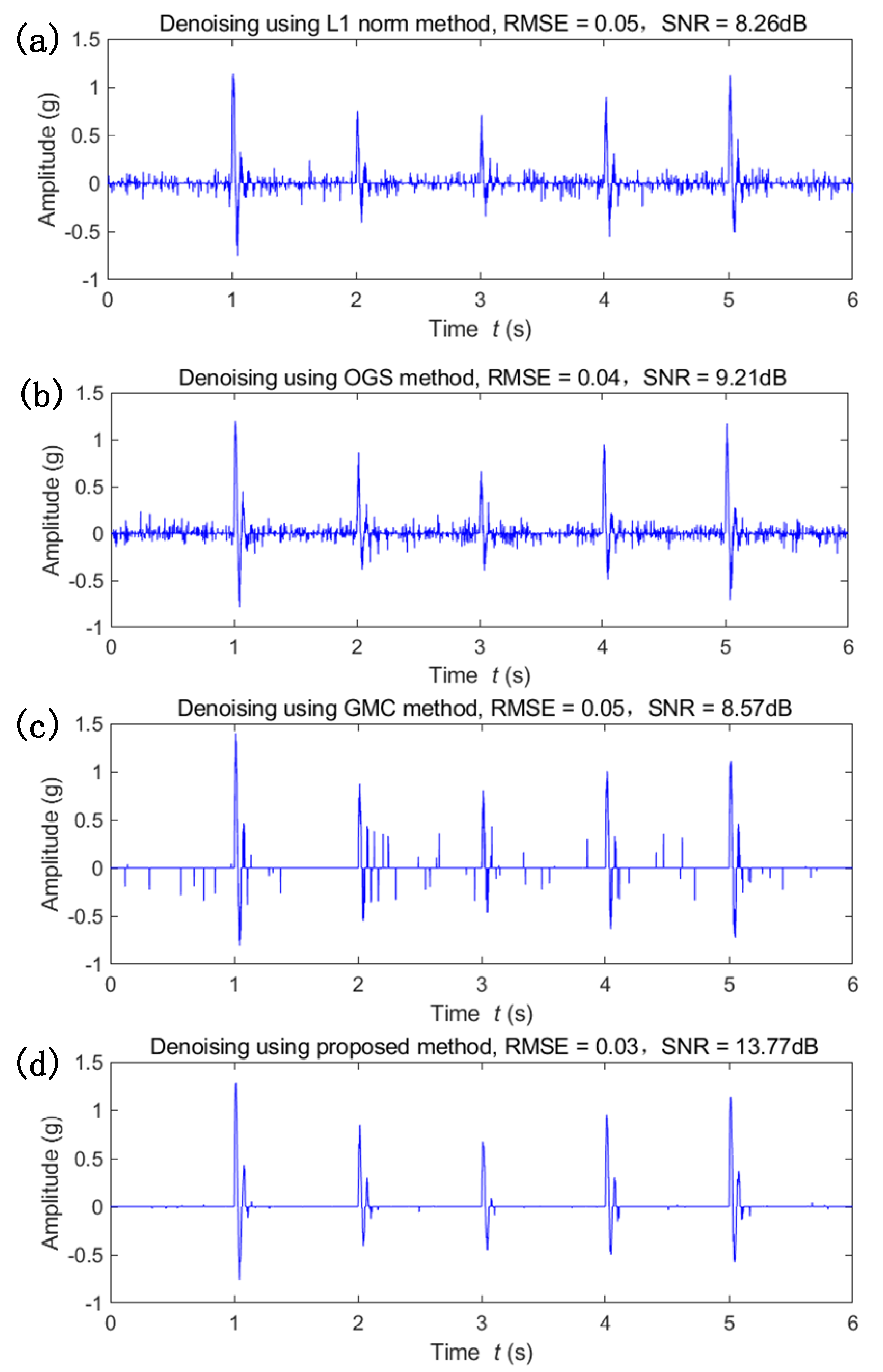
Previous signal-denoising methods have shown excellent performance in practical applications. In order to compare the previous methods and the proposed method with the SNR and RMSE, the best appropriate parameters λ and γ were selected for each method. The processed results obtained by the comparison methods and the proposed method are shown in Figure 4, respectively.
As shown in Figure 3 and Figure 4, compared with the 𝓁 1 norm regularization method, the OGS method and the original GMC penalty method, the performance of the proposed method is greatly improved. In particular, the 𝓁 1 norm regularization and GMC penalty method have a less satisfactory performance, and the proposed method has the best performance. From the perspective of the SNR and RMSE, the growth in performance using the proposed method is about twenty percent. The proposed method preserves large amplitudes of useful features and enhances the sparsity of the signal.

4.2. Selection of Regularization Parameter

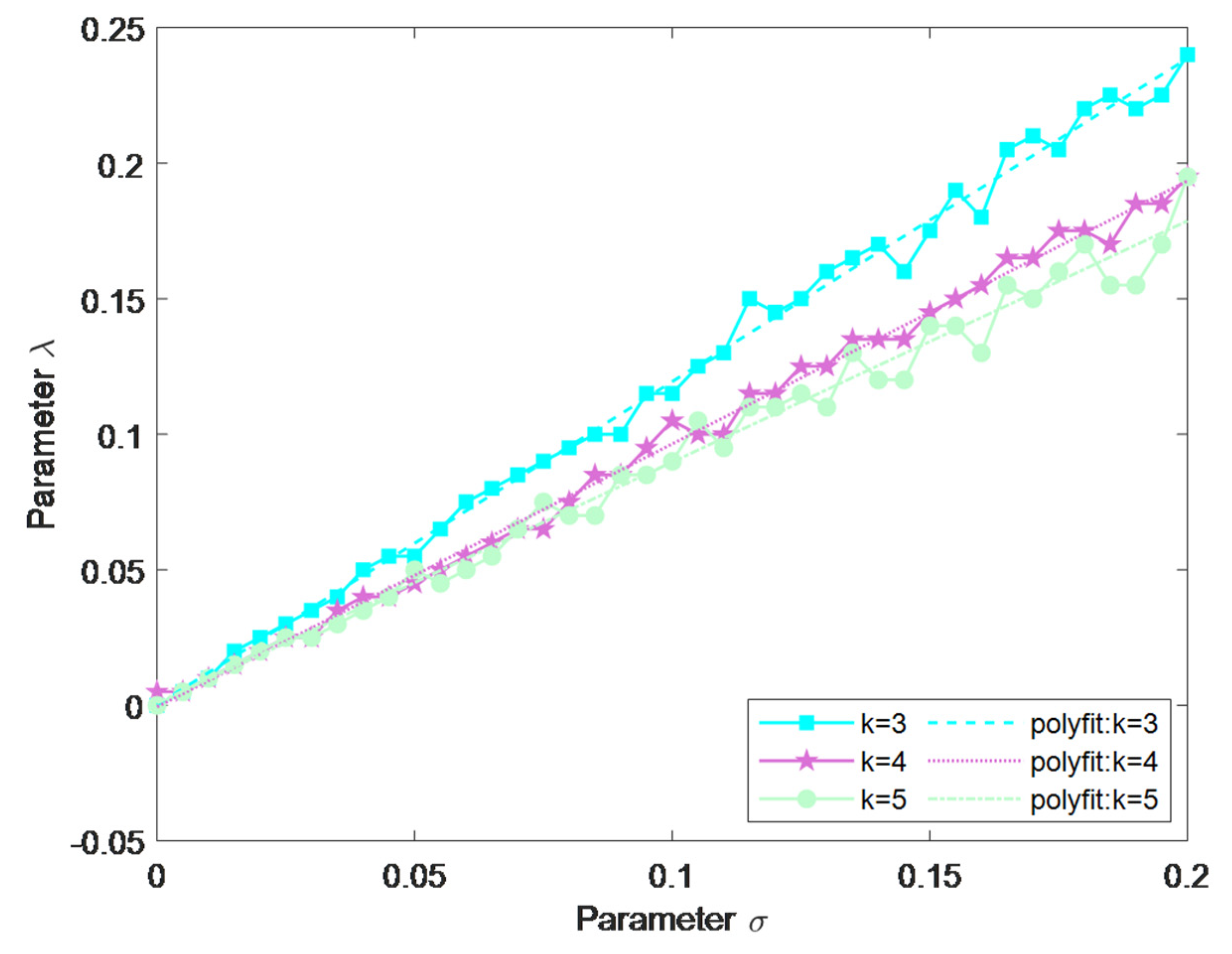
In this subsection, the criterion of selecting the regularization parameter is studied. In practice, the regularization parameter λ is suggested to be specified in proportion to the noise level, which is generally represented by the standard deviation σ of the noise in the signal [23]. The optimal regularization parameter λ as a function of the standard deviation σ using different group size K is displayed in Figure 4. Notice that the optimal value of the regularization parameter λ is obtained by minimizing the SNR of each fixed group size. Therefore, the regularization parameter λ can be specified by the straight line, which is fitted by numerical validation as illustrated in Figure 5.

5. Experimental Validation

In this section, the proposed group-sparse feature extraction method is applied to two experimental fault diagnosis cases to further demonstrate its performance. These two experimental cases correspond to a high-speed bearing and a pinion gear with faults, which are two key transmission components of wind turbines. The first diagnostic case is an outer-race fault induced in a high-speed bearing, while the other diagnostic case is a pinion gear with faults. The proposed method is applied to analyze measured noisy vibration signals, wherein the acceleration sensor was mounted radially to the high-speed shaft on the gearbox bearing support.

5.1. Case 1: High-Speed Bearing Outer-Race Fault

In this case, the proposed method is applied to analyze the vibration signals measured from a high-speed shaft bearing with a processed outer-race defect. Specifically, the vibration signal is radially measured on the bearing housing of a machinery-fault-simulator test rig. The sampling frequency is specified as 51.2 KHz and the rotating frequency is approximately f r = 29 Hz. For the tested bearing, the bearing type is MB ER-16K and the number of balls is nine. Meanwhile, the ball diameter is 7.9375 mm, and the pitch diameter is 38.50 mm. Based on the geometric parameters and rotational speed, the characteristic frequency of the outer-race defect is calculated to be approximately f o = 103.59 Hz [37].
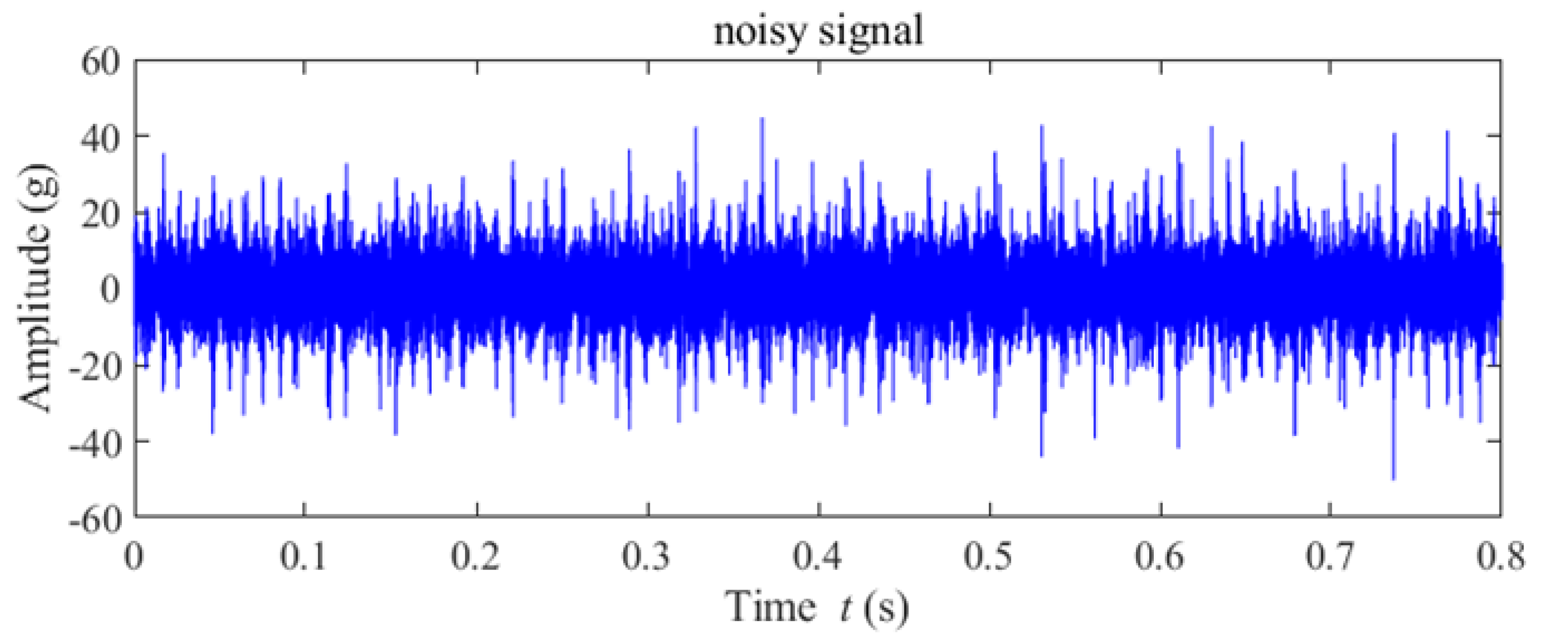
A record of the collected signal is shown in Figure 6, and it can be observed that the useful fault features are buried in strong background noise and irrelevant interference. In order to extract fault transients, the proposed method is applied to analyze the noisy signal. In this case, the processing result and its Hilbert envelop spectrum are shown in Figure 7. It can be observed from Figure 7a that the proposed method can reduce the background noise and extract the transients from the measured vibration data effectively. The Hilbert envelope spectrum of the extracted signal is illustrated in Figure 7b. It can be observed that the outer-race defect frequency f o = 103.59 Hz and its harmonic components are clearly revealed. Therefore, the fault features are effectively extracted in this case, which indicates that a localized outer-race fault occurred on the bearing.
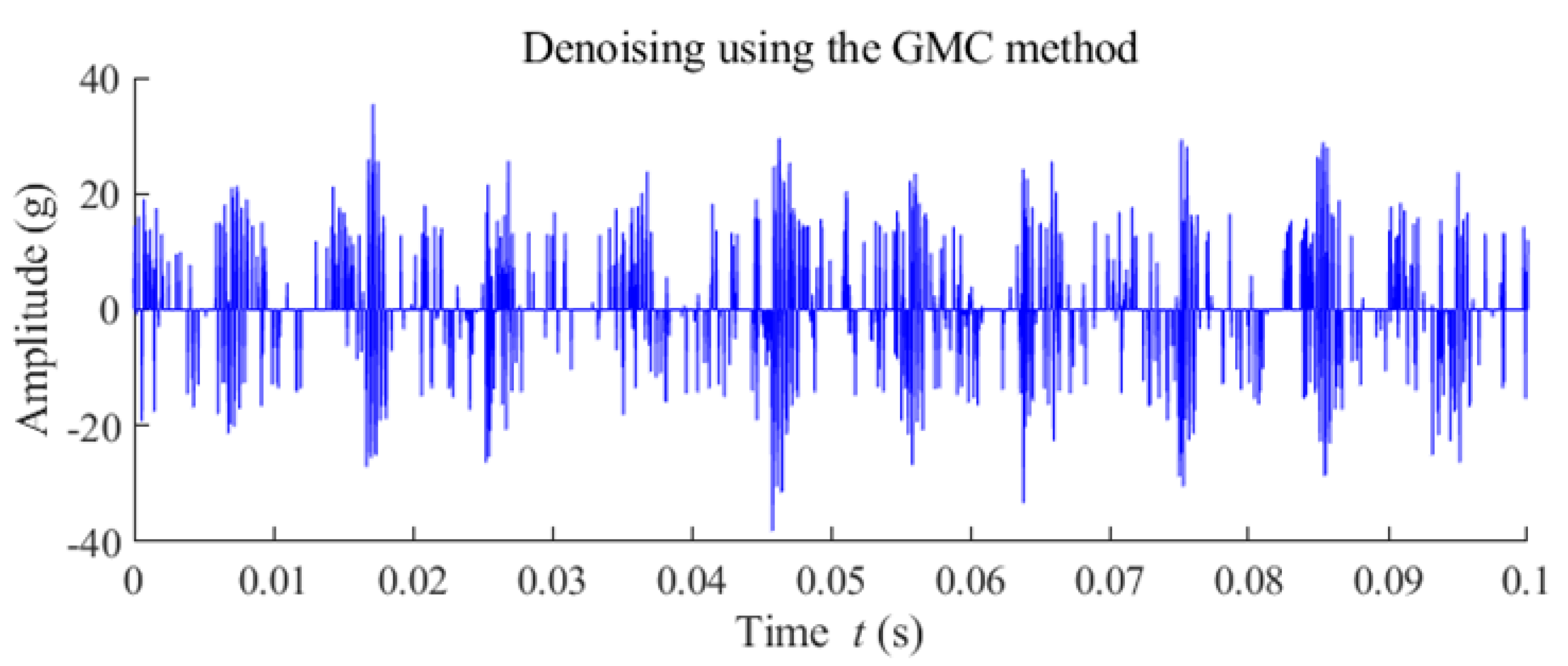
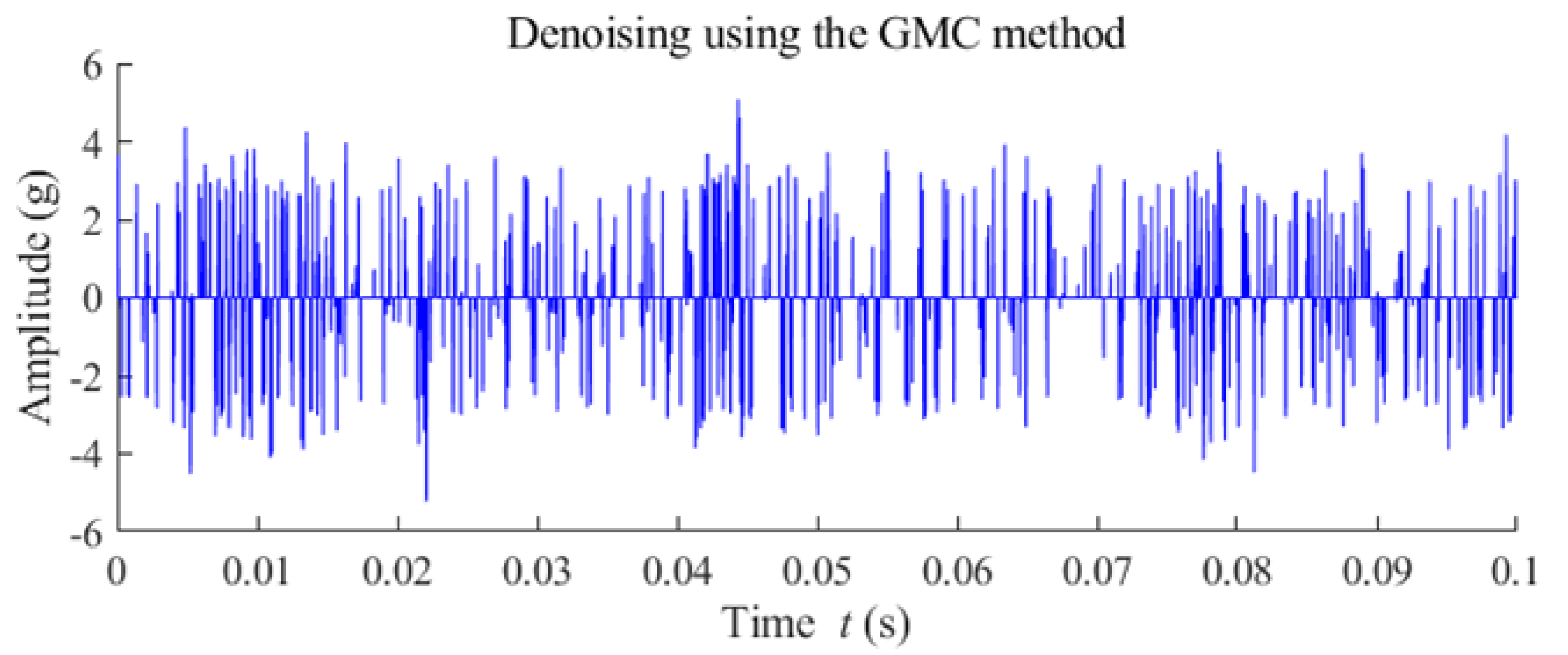
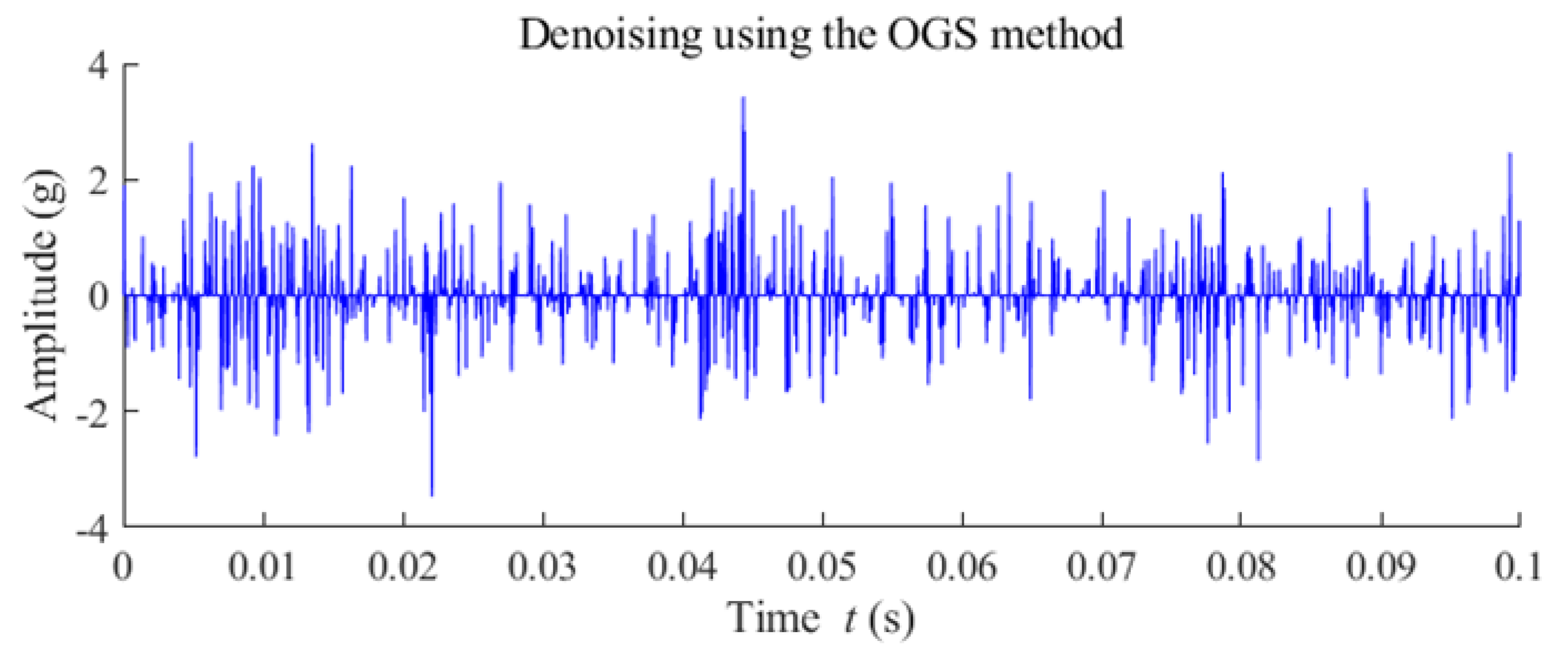
Similarly, for further comparison, the noisy vibration signal is also processed by the original GMC method and the OGS method. Figure 8 and Figure 9 demonstrate the denoising results used by the GMC method and OGS method, respectively. It can be observed from the denoised results using the comparative methods that the weakest fault features have been extracted. However, these useful fault features are still surrounded by irrelevant noise.

5.2. Case 2: Fault Diagnosis of a Wind Turbine Pinion Gear

In this case, the proposed method is applied to analyze a noisy vibration signal to extract sparse fault features of a wind turbine pinion gear. The radial vibration of a 3 MW wind turbine pinion was measured. The vibration signals were measured at a sampling frequency of 97.656 KHz. The rotating frequency (shaft frequency) was approximately f r = 30 Hz and the speed of the pinion gear shaft was approximately 1800 rpm. The number of teeth on the pinion was 32.
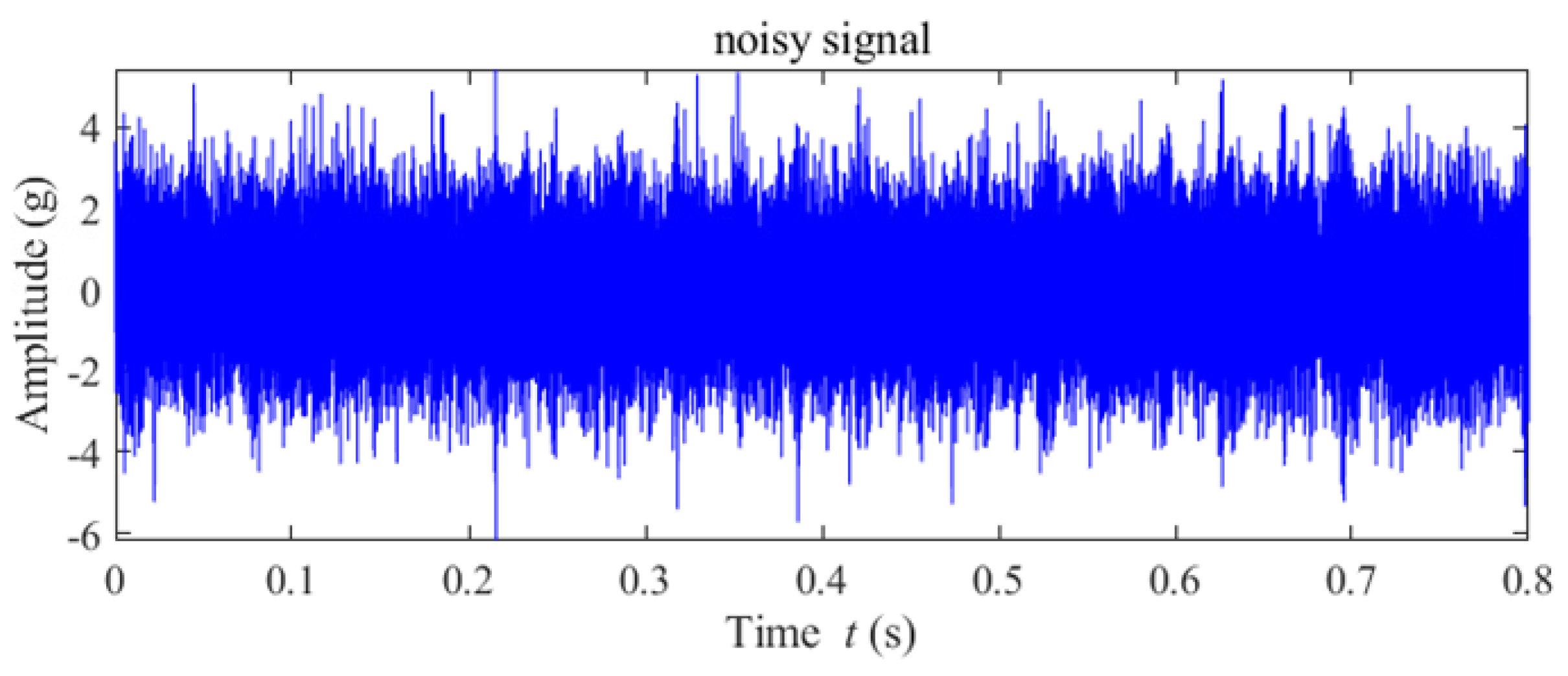
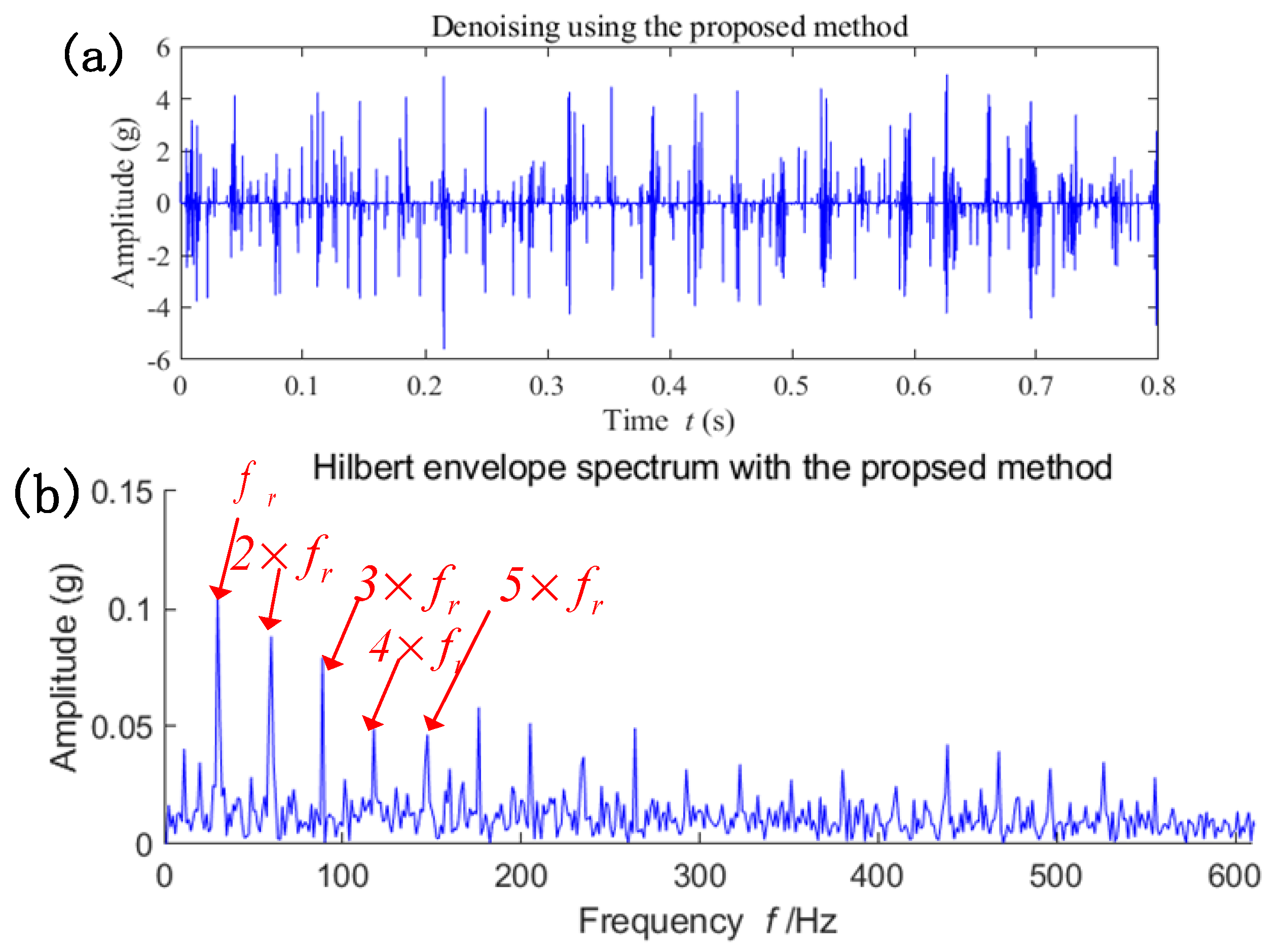
A record of the vibration signal is displayed in Figure 10. It can be seen that the fault features with group-sparse properties are masked by strong background noise and irrelevant interference. In order to estimate the fault transients more accurately, the proposed method is applied to analyze the measured noisy vibration signal. In this case, the optimal regularization parameter is specified as λ = 2.3 and the algorithm is run for 1000 iterations. The estimated result of the group-sparse transients and their Hilbert envelope spectrum are shown in Figure 11. It can be observed from Figure 11a that the repetitive transients with group-sparse properties are extracted from the measured vibration data. Specifically, the frequency of the group-sparse transients is approximately 30 Hz, which is in accordance with the rotating frequency f r of the pinion gear shaft. The Hilbert envelope spectrum of the extracted group-sparse signal is illustrated in Figure 11b. It can be observed that the rotating frequency of the pinion gear shaft is f r = 30 Hz. Therefore, in this case, the fault features with group-sparse properties have been effectively extracted, indicating that there is a local fault in the wind turbine pinion.
For comparison, the noisy vibration signal is processed by the GMC method. The estimated periodic group-sparse signal using the original GMC method is displayed in Figure 12. The useful transients are not estimated in a sparse way, wherein the interference noise still exists. For further comparison, the noisy vibration signal is also processed by the OGS method. In this experimental case, the extracted result obtained via OGS is illustrated in Figure 13. Similarly, although a few transients with large magnitudes can be revealed, the decomposed results are still noisy and the high-amplitude components are severely underestimated.

6. Conclusions

This paper proposes a data-driven sparse fault feature extraction method for wind turbine condition monitoring and fault diagnosis. Specifically, the proposed diagnostic method is based on the ensemble generalized minimax-concave penalty to maximally enhance the sparsity of useful weak fault features. The proposed method formulates weak fault features as group-sparse features, i.e., large useful magnitude values are not isolated. Therefore, the proposed method addresses the problem existing in the original GMC-based sparse feature extraction method. An effective unconstrained optimization problem is formulated, wherein the group-sparse structure is incorporated into non-convex regularization. Furthermore, the convex condition is derived to guarantee the convexity of the whole cost function of the optimization problem. The setting criteria of the regularization parameter of the proposed method is thoroughly investigated. The diagnostic performance of the proposed method is verified via numerical signals and experimental data collected from wind turbines. The extracted useful fault features demonstrate that the proposed method can effectively detect group-sparse weak fault features from noisy signals. Based on the sparse fault features extracted by the proposed method in this paper, future work will focus on formulating a quantitative index to precisely reveal the damage site and size of defective components.

Author Contributions

Conceptualization, W.H.; methodology, P.Z. and X.L.; validation, X.L.; investigation, P.Z.; writing—original draft, P.Z. and X.L.; writing—review & editing, X.L. and B.G.; supervision, W.H. and B.C.; funding acquisition, W.H. All authors have read and agreed to the published version of the manuscript.

Funding

This research is supported financially by the National Key R&D Program of China (Grant No. 2020YFB1713500), National Natural Science Foundation of China (Grant No.51805398), the Project of Youth Talent Lift Program of Shaanxi University Association for Science and Technology (Grant No. 20200408), and the Fundamental Research Funds for the Central Universities (Grant No. JB211303).

Institutional Review Board Statement

Not applicable.

Informed Consent Statement

Not applicable.

Data Availability Statement

This study did not report any data.

Conflicts of Interest

The authors declare no potential conflict of interest with respect to the research, authorship and/or publication of this article.

References

  1. Wang, M.-H.; Lu, S.-D.; Hsieh, C.-C.; Hung, C.-C. Fault Detection of Wind Turbine Blades Using Multi-Channel CNN. Sustainability 2022, 14, 1781. [Google Scholar] [CrossRef]
  2. Wang, X.; Tang, G.; Wang, T.; Zhang, X.; Peng, B.; Dou, L.; He, Y. Lkurtogram Guided Adaptive Empirical Wavelet Transform and Purified Instantaneous Energy Operation for Fault Diagnosis of Wind Turbine Bearing. IEEE Trans. Instrum. Meas. 2020, 70, 1–19. [Google Scholar] [CrossRef]
  3. Liu, X.; Ma, H.; Liu, Y. A Novel Transfer Learning Method Based on Conditional Variational Generative Adversarial Networks for Fault Diagnosis of Wind Turbine Gearboxes under Variable Working Conditions. Sustainability 2022, 14, 5441. [Google Scholar] [CrossRef]
  4. Yang, S.; Wang, Y.; Li, C. Wind turbine gearbox fault diagnosis based on an improved supervised autoencoder using vibration and motor current signals. Meas. Sci. Technol. 2021, 32, 114003. [Google Scholar] [CrossRef]
  5. He, W.; Guo, B.; Chen, B.; Ye, J.; Bechhoefer, E. A data-driven group-sparse feature extraction method for fault detection of wind turbine trans-mission system. Meas. Sci. Technol. 2020, 31, 074008. [Google Scholar] [CrossRef]
  6. Wang, C.; Gan, M.; Zhu, C. Intelligent fault diagnosis of rolling element bearings using sparse wavelet energy based on over-complete DWT and basis pursuit. J. Intell. Manuf. 2017, 28, 1377–1391. [Google Scholar] [CrossRef]
  7. He, Q.; Wang, X. Time-frequency manifold correlation matching for periodic fault identification in rotating machines. J. Sound Vib. 2013, 332, 2611–2626. [Google Scholar] [CrossRef]
  8. Zhang, D. Wavelet transform. In Fundamentals of Image Data Mining; Springer: Cham, Switzerland, 2019; pp. 35–44. [Google Scholar]
  9. Pathak, R.S. The Wavelet Transform; Springer Science & Business Media: Cham, Switzerland, 2009. [Google Scholar]
  10. Liu, C.-L. A Tutorial of the Wavelet Transform; NTUEE: Taiwan, China, 2010. [Google Scholar]
  11. Wang, L.-H.; Zhao, X.P.; Wu, J.X.; Xie, Y.-Y.; Zhang, Y.-H. Motor fault diagnosis based on short-time Fourier transform and convolutional neural network. Chin. J. Mech. Eng. 2017, 30, 1357–1368. [Google Scholar] [CrossRef]
  12. Zhong, J.; Huang, Y. Time-Frequency Representation Based on an Adaptive Short-Time Fourier Transform. IEEE Trans. Signal Process. 2010, 58, 5118–5128. [Google Scholar] [CrossRef]
  13. Li, Z.; Jiang, Y.; Guo, Q.; Hu, C.; Peng, Z. Multi-dimensional variational mode decomposition for bearing-crack detection in wind turbines with large driving-speed variations. Renew. Energy 2016, 116, 55–73. [Google Scholar] [CrossRef]
  14. Li, Z.; Liu, F.; Sun, S.; Sarkodie-Gyan, T.; Li, W. Decoupling of Multiple Concurrent Faults for Diagnosing Coal-cutter Gearboxes: An Extensive Ex-perimental Investigation with Multi-Channel Sensor Measurements. Nondestruct. Eval. Diagn. Progn. Eng. Syst. 2019, 2, 041001. [Google Scholar]
  15. Xiang, J.; Zhong, Y.; Gao, H. Rolling element bearing fault detection using PPCA and spectral kurtosis. Measurement 2015, 75, 180–191. [Google Scholar] [CrossRef]
  16. Liu, W.Y.; Gao, Q.W.; Ye, G.; Ma, R.; Lu, X.N.; Han, J.G. A novel wind turbine bearing fault diagnosis method based on Integral Extension LMD. Measurement 2015, 74, 70–77. [Google Scholar] [CrossRef]
  17. Lei, Y.; Qiao, Z.; Xu, X.; Lin, J.; Niu, S. An underdamped stochastic resonance method with stable-state matching for incipient fault diagnosis of rolling element bearings. Mech. Syst. Signal Process. 2017, 94, 148–164. [Google Scholar] [CrossRef]
  18. He, Q.; Wu, E.; Pan, Y. Multi-Scale Stochastic Resonance Spectrogram for fault diagnosis of rolling element bearings. J. Sound Vib. 2018, 420, 174–184. [Google Scholar] [CrossRef]
  19. Buzzoni, M.; Antoni, J.; d’Elia, G. Blind deconvolution based on cyclostationarity maximization and its application to fault iden-tification. J. Sound Vib. 2018, 432, 569–601. [Google Scholar] [CrossRef]
  20. Wan, S.; Zhang, X.; Dou, L. Compound fault diagnosis of bearings using improved fast spectral kurtosis with VMD. J. Mech. Sci. Technol. 2018, 32, 5189–5199. [Google Scholar] [CrossRef]
  21. Wang, Y.; Xiang, J.; Markert, R.; Liang, M. Spectral kurtosis for fault detection, diagnosis and prognostics of rotating machines: A review with applications. Mech. Syst. Signal Process. 2016, 66–67, 679–698. [Google Scholar] [CrossRef]
  22. Tsai, T.C.; Wang, C.N. Acoustic-based method for identifying surface damage to wind turbine blades by using a convolutional neural network. Meas. Sci. Technol. 2022, 33, 085601. [Google Scholar] [CrossRef]
  23. Ding, C.; Zhao, M.; Lin, J. Sparse feature extraction based on periodical convolutional sparse representation for fault detection of rotating machinery. Meas. Sci. Technol. 2020, 32, 015008. [Google Scholar] [CrossRef]
  24. Song, Z.; Huang, W.; Liao, Y.; Mao, L.; Shi, J.; Wang, J.; Shen, C.; Zhu, Z. Sparse representation based on generalized smooth logarithm regularization for bearing fault diagnosis. Meas. Sci. Technol. 2021, 32, 105003. [Google Scholar] [CrossRef]
  25. Wang, L.; Zhang, X.; Liu, Z.; Wang, J. Sparsity-based fractional spline wavelet denoising via overlapping group shrinkage with non-convex regularization and convex optimization for bearing fault diagnosis. Meas. Sci. Technol. 2019, 31, 055003. [Google Scholar] [CrossRef]
  26. Hai, B.; Jiang, H.; Yao, P.; Wang, K.; Yao, R. Rolling bearing fault feature extraction using non-convex periodic group sparse method. Meas. Sci. Technol. 2021, 32, 105005. [Google Scholar] [CrossRef]
  27. Xia, Y.; Lu, S. Convolutional sparse coding with periodic overlapped group sparsity for rolling element bearing fault diagnosis. Meas. Sci. Technol. 2018, 29, 115103. [Google Scholar] [CrossRef]
  28. Chen, P.Y.; Selesnick, I.W. Translation-invariant shrinkage/thresholding of group sparse signals. Signal Process. 2014, 94, 476–489. [Google Scholar] [CrossRef] [Green Version]
  29. Chen, P.Y.; Selesnick, I.W. Group-sparse signal denoising: Non-convex regularization, convex optimization. IEEE Trans. Signal Process. 2014, 62, 3464–3478. [Google Scholar] [CrossRef] [Green Version]
  30. Huang, W.; Sun, H.; Wang, W. Resonance-Based Sparse Signal Decomposition and Its Application in Mechanical Fault Diagnosis: A Review. Sensors 2017, 17, 1279. [Google Scholar] [CrossRef] [Green Version]
  31. Fan, W.; Cai, G.; Huang, W.; Shang, L.; Zhu, Z. Sparse Representation of Transients Based on Wavelet Basis and Majorization-Minimization Algorithm for Machinery Fault Diagnosis. Math. Probl. Eng. 2014, 2014, 696051. [Google Scholar] [CrossRef] [Green Version]
  32. He, W.; Ding, Y.; Zi, Y.; Selesnick, I.W. Repetitive transients extraction algorithm for detecting bearing faults. Mech. Syst. Signal Process. 2017, 84, 227–244. [Google Scholar] [CrossRef] [Green Version]
  33. Selesnick, I. Sparse Regularization via Convex Analysis. IEEE Trans. Signal Process. 2017, 65, 4481–4494. [Google Scholar] [CrossRef]
  34. He, W.; Hu, J.; Chen, B.; Guo, B. GMC sparse enhancement diagnostic method based on the tunable Q-factor wavelet transform for detecting faults in rotating machines. Measurement 2021, 174, 109001. [Google Scholar] [CrossRef]
  35. Liu, J.; Qiao, B.; He, W.; Yang, Z.; Chen, X. Impact force identification via sparse regularization with generalized minimax-concave penalty. J. Sound Vib. 2020, 484, 115530. [Google Scholar] [CrossRef]
  36. He, W.; Chen, B.; Zeng, N.; Zi, Y. Sparsity-based signal extraction using dual Q-factors for gearbox fault detection. ISA Trans. 2018, 79, 147–160. [Google Scholar] [CrossRef]
  37. Randall, R.B.; Antoni, J. Rolling element bearing diagnostics—A tutorial. Mech. Syst. Signal Process. 2011, 25, 485–520. [Google Scholar] [CrossRef]
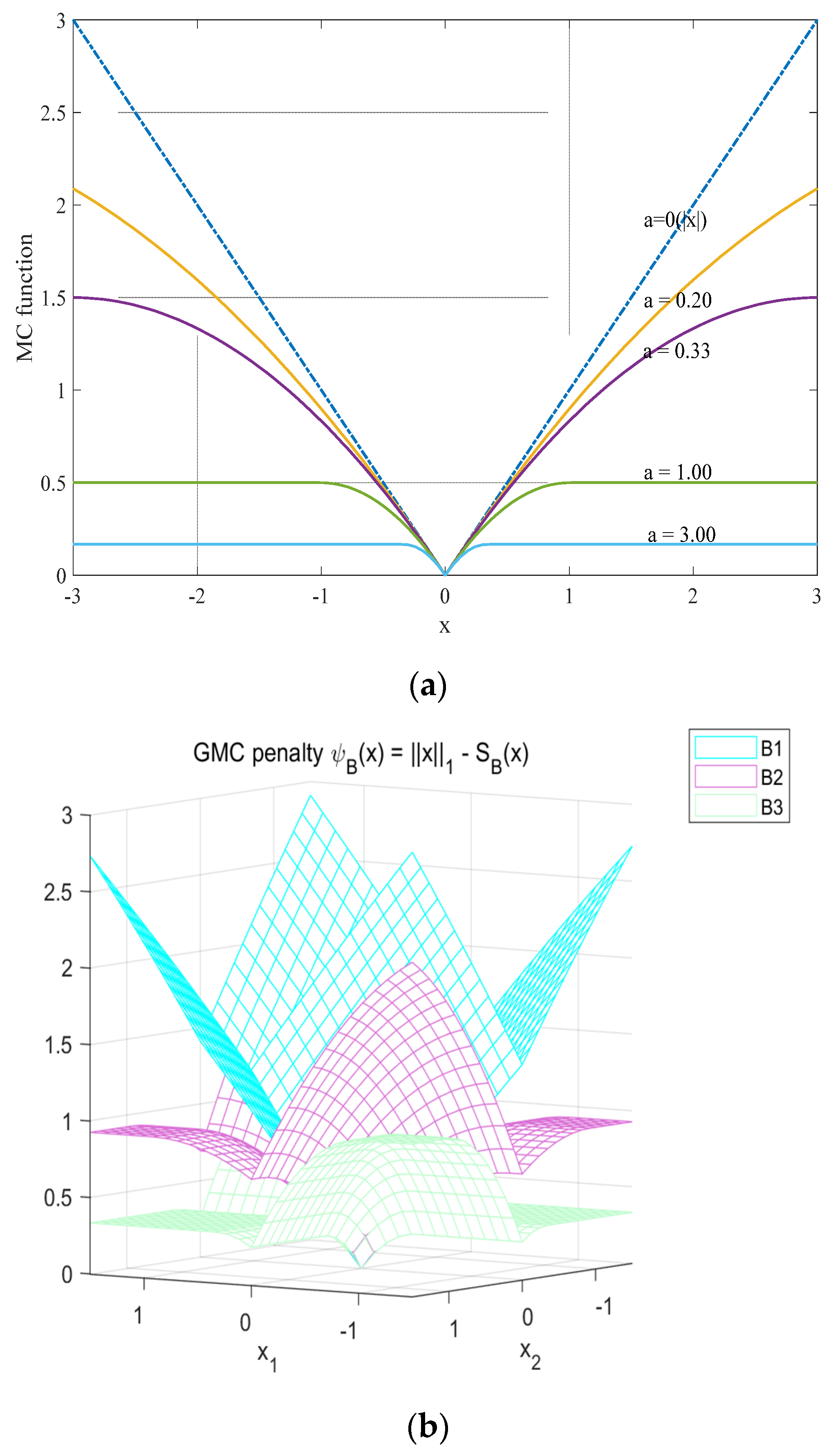
Figure 1. The non−convex degree of two functions varies with the parameter. (a) MC function. (b) GMC function.
Sustainability 14 16793 g001
Figure 2. The procedure of the proposed group−sparse feature extraction method.
Sustainability 14 16793 g002
Figure 3. Noise−free signal and noise signal. (a) Noise-free signal, (b) Noise signal with Gaussian noise of σ = 0.1 .
Sustainability 14 16793 g003
Figure 4. Denoising results obtained using the comparison methods and proposed method. (a) Denoising using 𝓁 1 norm regularization with λ = 0.14 . (b) Denoising using OGS method with λ = 0.07 . (c) Denoising using GMC penalty with λ = 0.26 and γ = 0.8 . (d) Denoising using the proposed method with λ = 0.15 , γ = 0.8 and K = 3 .
Sustainability 14 16793 g004
Figure 5. Optimal regularization parameter at different noise levels.
Sustainability 14 16793 g005
Figure 6. Measured noisy signal.
Sustainability 14 16793 g006
Figure 7. (a) Extracted transient signal. (b) Hilbert envelope spectrum of the signal.
Sustainability 14 16793 g007
Figure 8. Extracted group−sparse signal using the original GMC method.
Sustainability 14 16793 g008
Figure 9. Extracted group−sparse signal using the OGS method.
Sustainability 14 16793 g009
Figure 10. Measured noisy signal.
Sustainability 14 16793 g010
Figure 11. (a) Extracted transient signal. (b) Hilbert envelope spectrum of the signal.
Sustainability 14 16793 g011
Figure 12. Extracted group−sparse signal using the original GMC method.
Sustainability 14 16793 g012
Figure 13. Extracted group−sparse signal using the OGS method.
Sustainability 14 16793 g013
Publisher’s Note: MDPI stays neutral with regard to jurisdictional claims in published maps and institutional affiliations.