A New Decision Framework of Online Multi-Attribute Reverse Auctions for Green Supplier Selection under Mixed Uncertainty

Abstract

In order to realize the “dual carbon” goal proposed for the world and to seek the low-carbon and sustainable development of the economy and society, the green supply chain management problem faced by Chinese enterprises and governments is particularly important. At the same time, how to quickly and efficiently select the suitable green supplier is the most basic and critical link in green supply chain management, as well as an important issue that Chinese government and enterprises must face in the process of green material procurement. In addition, there are various uncertainties emerging in the current market environment that hinder the green suppliers and the buyer to make the efficient decisions. Therefore, in order to find a more suitable and efficient method for green supplier selection, from the standpoint of the buyer, a new decision framework of online multi-sourcing, multi-attribute reverse auction (OMSMARA), which effectively improves the procurement efficiency and reduces procurement costs and risks, is proposed under the mixed uncertainty. Specifically, the main innovation work includes three aspects: Firstly, the trapezoidal fuzzy numbers are applied to describe the uncertain bidding attribute values by the green suppliers. Secondly, the hesitant fuzzy sets theory is introduced to characterize the buyer’s satisfaction degrees of the bidding evaluation attribute information, and the attribute weights are determined by using the hesitant fuzzy maximizing deviation method. Thirdly, a fuzzy multi-objective mixed integer programming model is proposed to solve the green supplier selection and quantity allocation question in OMSMARA. A numerical example is given to demonstrate the feasibility and effectiveness of the proposed decision framework, and the sensitivity analysis and comparison analysis further show the robustness and reliability of the proposed solution method.

1. Introduction

In recent years, due to climate change and carbon emissions [1,2,3,4,5,6], environmental pollution has seriously increased, which is contrary to the concept of sustainable development. Prosperity and beauty are closely connected with green development in China, which shows the significance of implementing a green supply chain management [7]. Furthermore, in the green supply chain management, selecting the green supplier is most vital [8]. A green supplier with high quality not only reduces the cost, but also performs well in pro-environment. It adopts green action, introduces green skills talents, and creates green products, which will make the related enterprises or companies more competitive, with more benefits [9,10]. Therefore, what effective green supplier selection methods should be selected by governments and enterprises, and what are the important criteria for how to identify the appropriate green suppliers are the key issues that need to be addressed urgently.

Currently, it is not difficult to find that there are several Internet trading platforms, such as eBay, Onsale, and Taobao, serving for both B2C and B2B markets. At the same time, online auction has grown to be a convenient, low-cost, and low-carbon way of commodity trading for the traders [11,12]. Usually, online auctions include online forward auctions and online reverse auctions (ORA). Opposite to the online forward auctions, ORA is implemented in a situation where a buyer requests the quotes from multiple qualified suppliers [13]. However, traditional ORA only consider price as the evaluation factor, but neglect other important green attributes, such as product quality, delivery time, after-sales service level, etc. Ignoring such attributes may cause serious losses sometimes [14]. The online multi-attribute reverse auctions (OMARA) that can effectively make up for the above deficiencies are widely used in government procurement and project bidding [15,16]. In addition, most existing OMARA literature focused on the case referred to as sole-sourcing auctions, in that determining only one winner by various methods. However, there are few auction literature studied the multi-sourcing situation. Obviously, due to the complex market environment and various potential risks, the sole-sourcing auction may cause serious consequences when the winner breaks a contract [17]. On the contrary, online multi-sourcing, multi-attribute reverse auction (OMSMARA) is more in line with practical needs, which not only reduces the risk, but also help build a few friendly market partnerships. For example, IBM carried out a multi-sourcing reverse auction for purchasing a large quantity of chairs for one office building and achieved very good benefits [18]. So, in this paper, we focus on OMSMARA and its application for green supplier selection.

At the same time, various uncertainties are emerging in the current procurement auction market environment [19,20], which make the ideal hypotheses of traditional auction theory hardly in line with the reality. This will make it difficult for suppliers (bidders) and purchasers (auctioneers) to execute the relevant decision-makings. For instance, the purchaser is required to determine the attribute requirements of the goods and the corresponding importance of these attributes. Additionally, the buyer needs to choose the evaluation method to conduct a comprehensive evaluation of the suppliers’ bids. So, the suppliers have to properly describe the information of the attribute values in the bids under an uncertain environment. According to [14,21], we find that the general fuzzy set theory, including interval number, trapezoidal fuzzy numbers (TrFN), and semantic fuzzy set, was introduced to the winner determination of the bidding supplier in OMARA and effectively dealt with the uncertainty.

In the selection of green suppliers using OMSMAR, relevant participants often face the following important problems: (1) How to effectively depict the relevant uncertainty information in the selection and decision problem of green suppliers. (2) When the purchaser cannot directly determine the accurate weight of bidding evaluation attributes, what effective weight determination method should be adopted? (3) Based on the previous obtained information, it is important to determine how to build the green supplier procurement auction optimization model to solve the problems of supplier winner determination and the corresponding order quantity allocation at the same time, which specifically involves the construction of relevant models, model transformation, and model solution problems. Therefore, in order to find a more suitable and efficient method for green supplier selection under the mixed uncertainty, from the standpoint of the buyer, a new decision framework of online multi-sourcing, multi-attribute reverse auction (OMSMARA), which effectively improves the procurement efficiency and reduce procurement costs and risks, is proposed.

There are several possible innovations in the decision framework of OMSMARA for green supplier selection under mixed uncertainty: (1) Considering various uncertainties in the market environment, green suppliers can describe the bidding attribute values by TrFN. (2) To deal with the auctioneer’s (buyer’s) hesitant uncertainty in the auction, we introduce the hesitant fuzzy sets (HFE) to characterize the satisfaction degree values of relevant attributes information on each bid. To the best of our knowledge, this maybe the first time to apply the hesitant fuzzy set theory to the OMSMARA. (3) We consider both the subjective and objective bidding information to determine the synthetic attribute weights by HF-MDM. (4) Considering the buyer’s budget constraint, suppliers’ capacity constraints, and other uncertainties, we formulate a fuzzy multi-objective mixed integer programming model to solve the green supplier selection and quantity allocation questions in the OMSMARA. (5) To make this research more practical, we take into account the multiple-type preferences of the decision-maker, such as distance preference and objective weight preference.

The rest of the paper is organized as follows. Section 2 presents the relevant literature related to this research. Some preliminaries about HFS and TrFN are proposed in Section 3. In Section 4, we describe the flowchart of OMSMARA and introduce the decision question of the paper. Then, we propose decision framework of OMSMARA for green supplier selection under mixed uncertainty and demonstrate how to determine the attributes’ weight and selecting the winning green suppliers in Section 5. A fuzzy multi-objective mixed-integer programming model is formulated for solving the decision-making problems of the buyer in the OMSMARA in Section 6. In Section 7, a numerical example is provided to validate the effectiveness and applicability of the proposed decision framework of OMSMARA for green supplier selection. In Section 8, we present the sensitivity analysis of the relevant model parameters and provide a comparative analysis to show our proposed framework with the other two methods. Lastly, we conclude this study, and possible future research directions are put forward.

2. Literature Review

In this section, we collate the literature related to this study from three aspects and indicate the connections and differences between the study contents in this paper.

2.1. Multi-Attribute Reverse Auctions (MARA) and Its Extentions

For the MARA and OMARA, Che [22] studied them systematically for the first time. Subsequently, David et al. [23] extended the English auction to the English MARA. However, Bellosta et al. [24] pointed out the difficulty of OMARA is determining the bidding attribute weight. Teich et al. [11] proposed a mathematical programming approach, and Cheng et al. [25] used the TOPSIS (technique for order preference by similarity to ideal solution) method to determine the attribute weight in MARA. In addition, there is much application research about MARA, for example, Hu et al. [26] proposed an incentive mechanism in mobile crowdsourcing based on MARA. Jain et al. [27] applied MARA to supplier selection for two-way competition in oligopoly market of supply chain. Long et al. [15] provided an overview of OMARA that the readers can refer to.

Apparently, the above works only considered quantitative attributes with the determined values. To extend related research, Singh et al. [28] used the F-TOPSIS method to evaluate the bidding suppliers from both the quantitative and qualitative perspectives. Qian et al. [29] proposed a winner determination method for clean energy device procurement by MARA when the buyer is loss-averse and with incomplete information. Wang et al. [30] proposed an integrated multi-stage, decision-making framework for the winner determination problem in OMARA under mixed uncertainty. In this paper, we further extend OMARA to OMSMARA and study how to effectively apply them to the procurement auction process of green supplier selection.

2.2. Supplier Selection and Green Supplier Selection

The (green) supplier selection is key to the effective (green) procurement management [31,32,33,34,35,36], which includes a single sourcing format and multiple sourcing one. For the former, the decision-maker (buyer) needs to make only one decision. However, for the latter, the buyer will assign the purchase quantities to multiple suppliers when a single supplier cannot meet the requirements in a complex and volatile market environment [32,33]. Currently, there are a lot of studies on (green) supplier selection. For example, Rao et al. [33] studied the supplier selection problem by multi-source procurement for coal. Bohner et al. [34] studied the supplier selection under failure risk and different discounts by using mixed-integer linear programming. Meanwhile, Cheraghalipour et al. [35] proposed a decision framework to solve the sustainable (green) supplier selection problem under a multi-period, multi-item, and multi-supplier situation. In addition, Assellaou et al. [36] developed a new stochastic multi-objective optimization model for supplier selection and order allocation under multiple uncertainties.

All the above studies considered various situations and different methods to deal with supplier selection and quantity allocation questions. However, there is limited literature on using OMSMARA for green supplier selection, and even fewer studies considering more green attribute guidelines and complex uncertain situations. To this end, we study the decision-making problem of OMSMARA for green supplier selection under mixed uncertainty in this study.

2.3. Hesitant Fuzzy Sets (HFS) and Its Applications

Due to the complexity of the decision-making environment and the inherent vagueness of human preferences, people are usually hesitant and indecisive when they express their views or evaluations. To cope with this problem, Torra et al. [37] proposed the HFS to expand the traditional fuzzy set theory. Subsequently, many studies, such as [38,39,40,41], concentrated on the research of the HFS extensions and their applications. All the studies above indicated that, when representing human hesitant uncertainty and ambiguity, HFS can behave more objectively and effectively than other classical and extended fuzzy sets.

However, In the field of auction and its application, limited literature considered the hesitant decision-making psychology of auctioneer (purchaser), and almost no literature has introduced HFS into the research of auction decision problem. Therefore, based on the advantages of HFS and the practical need of the auction decision-making problem that we study here, we introduce HFS theory into OMSMARA field and solve the problem of green supplier selection.

3. Preliminaries

In this section, some basic definitions and relevant concepts of HFSs and TrFNs are introduced to serve for the later research.

Definition 1

[39]. Let X be a finite universe of discourse, a HFS $E$ on X is defined in terms of a function, such that when it is applied to X, it returns a subset of [0,1]. It can be represented as follows.

$$E=\{<x,h_E(x)>|x\in X\}$$

(1)

where $h_E(x)$ is referred to a hesitant fuzzy element (HFE). Each HFE contains several numerical values that belong to [0, 1], representing the possible membership (or satisfaction degrees) of the element $x\in X$. $E$ is the set of all the HFEs. When arrange the HFEs in $h_E(x)$ in decreasing order, we let $h_E^{\delta \left\{l\right\}}(x)$ ($l=1,2,\cdots ,l{h}_E(x)$) be the l-th largest value, where $l{h}_E(x)$ is the number of values in $h_E(x)$. For simplicity, we denote $h_E(x)$ as $h(x)$ hereafter. The relevant calculation rules of HFE can refer to [40,41].

Definition 2

[42]. Let $lh(x_1)$ and $lh(x_2)$ denote the number of the HFEs $h(x_1)$ and $h(x_2)$, respectively. If $l{h}_1\ne l{h}_2$, (suppose $l{h}_1>l{h}_2$) the shorter one can be extended to the equal number by adding a certain number (i.e., $l{h}_1-l{h}_2$) of new value(s) with the form of ${\overline{h}}_2=\rho h_2^{+}+(1-\rho )h_2^{-}$, where $h_2^{+}$ and $h_2^{-}$ denote the max and min values of $h_2$, and $0\le \rho \le 1$ is the parameter determined by decision-maker’s risk preference, in which $\rho =0$ indicates risk-averse, $\rho =1$ indicates risk-seeking, and $\rho =0.5$ indicates risk-neutral.

Definition 3

[42]. The score function of a HFE h is defined as: $SF(h)={\displaystyle \sum _{r\in h}(\frac{r}{lh}})$, where lh denote the number of the elements in h. Moreover, the average deviation function is represented as: $D(h)=\frac{1}{lh}{\displaystyle \sum _{r\in h}(r-SF(h)}{)}^2$.

According to the above Definition 3, the comparison rules of a pair of HFEs are as follows:

(1)

If $SF(h_1)>SF(h_2)$, then $h_1>h_2$; If $SF(h_1)<SF(h_2)$, then $h_1<h_2$;

(2)

If $SF(h_1)=SF(h_2)$, then $D(h_1)>D(h_2)$, $h_1<h_2$; $D(h_1)=D(h_2)$, $h_1=h_2$; $D(h_1)<D(h_2)$, $h_1>h_2$.

Definition 4

[43]. Let $h_1$ and $h_2$ be two HFEs (without loss of generality, assume that they have the same number of elements, denoted by lh). The distance between $h_1$ and $h_2$ can be defined as follows:

$$d(h_1,h_2)={[\alpha d_1^{\lambda }+(1-\alpha )d_2^{\lambda }]}^{\frac{1}{\lambda }},0\le \alpha \le 1,\lambda >0.$$

(2)

where $d_1={[\frac{1}{lh}{\displaystyle \sum _{l=1}^{lh}|}{h}_1^{\delta (l)}-h_2^{\delta (l)}{|}^{\lambda }]}^{\frac{1}{\lambda }}$, $d_2={[ma{x}_l|h_1^{\delta (l)}-h_2^{\delta (l)}{|}^{\lambda }]}^{\frac{1}{\lambda }}$.

In (2), $\alpha$ denotes the buyer’s distance preference coefficient. $\alpha =0$ prefers the generalized Hausdorff distance, and $\alpha =1$ prefers the generalized Hamming distance, if $\alpha =0.5$ means equal importance for the above two kinds of distance.

Definition 5

[30]. A trapezoidal fuzzy number (TrFN) is denoted as $\tilde{a}=[a^1,a^2,a^3,a^4]$, and it has the following membership function:

$${\mu }_{\tilde{a}}(x)=\{\begin{array}{l}\frac{x-a^1}{a^2-a^1},a^1<x\le a^2;\\ {}_{}1,a^2<x\le a^3;\\ \frac{a^4-x}{a^4-a^3},a^3<x\le a^4;\\ {}_{}0,otherwise.\end{array}$$

(3)

where $a^1\le a^2\le a^3\le a^4$, and the basic comparison and calculation rules of TrFN can be refer to [44].

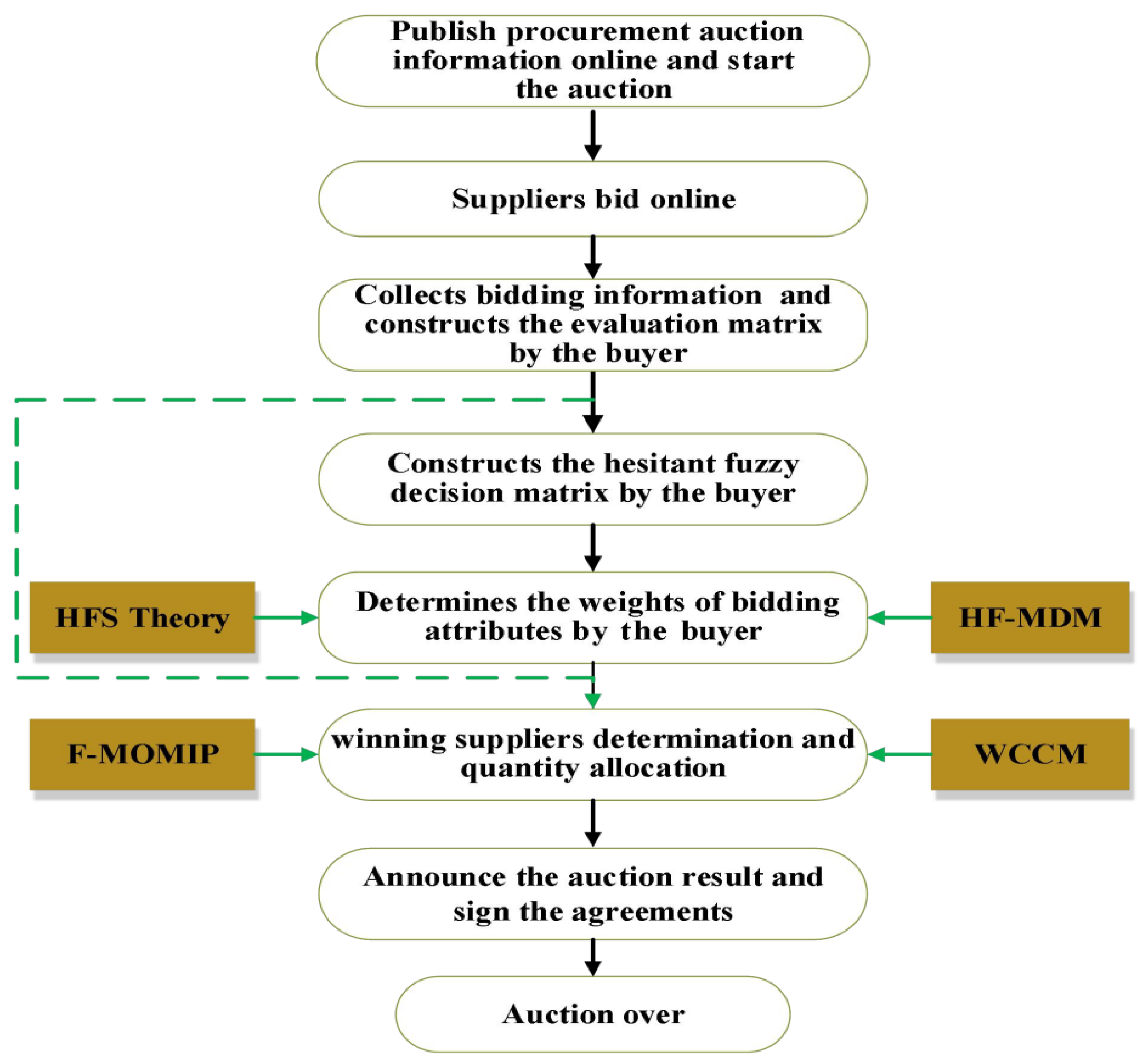
4. Description of the Online Multi-Sourcing Multi-Attribute Reverse Auction (OMSMARA)

Suppose a buyer (purchaser/auctioneer) intends to purchase a certain quantity of some commodity through ORA. Suppose there are m compliant green suppliers participating in the bidding process. The buyer announces the basic requirements of the purchased commodity, including price attribute and other non-price attribute indices, online. Simultaneously, according to the historical experience, the buyer identifies the key attributes (suppose the total number of attributes is n) for the evaluation of the bids. However, the buyer has uncertain information about the attribute weight.

After considering the changing market environment, unpredictable risk, and the buyer’s requirements, the suppliers’ uncertain bidding attribute values are described by using TrFNs. The buyer often faces some cognitive uncertainty and professional limitations, which often leads to an irresolute phenomenon in decision-making. Hence, we assume that the buyer takes HFS to depict the membership (or satisfaction) degree about the bidding attribute values. Then, the attribute weights can be calculated according to the constructed hesitant fuzzy decision matrix. Based on the obtained attribute weight and the suppliers’ bidding alternatives, the buyer determines the winning green suppliers and their quantity allocations.

As described above, the general processes of the OMSMARA can be as shown in Figure 1.

Among the above stages, the fifth and sixth stages are the most important parts in the OMSMARA. Therefore, in this paper, we mainly focus on the methods for dealing with the relevant decision-making questions in these two stages.

To simplify the analysis, some assumptions are made for the question formulation and model construction are given below:

①

It is assumed that the purchaser is taking a sealed OMARA, all the suppliers participating in the online auction bid truthfully and independently, and supposing that there is no collusion among them.

②

The buyer does not precisely know the importance of the relevant attributes of the product, and incomplete attribute weight information exists.

③

Due to the uncertain market environment and potential risks, it is assumed that each attribute values in the suppliers’ submitted bids are described by TrFNs.

④

Due to the limitation of cognition and specialty, the purchaser gives a preliminary evaluation value on the membership (satisfaction) degree that the attribute value of each bidding alternatives meets the requirement using HFS.

⑤

It is assumed that the reverse auction in this paper only considers the form of single-round auction. Multiple rounds and interactive situations are not considered temporarily.

⑥

It is assumed that the online procurement auction process generates a certain amount of setup cost for the buyer when signing the auction agreements with the winning bidders. We do not consider the auction participation fee of suppliers temporarily.

5. The Proposed Decision Framework of OMSMARA for Green Supplier Selection under Mixed Uncertainty

Based on the above description of the OMSMARA, in this paper, we introduce a new decision framework of OMSMARA to select the winning bidders (green suppliers) and their order allocations under mixed uncertainty. The processes of OMSMARA and the main content of the proposed decision framework are shown in Figure 1. Before entering into the details of the decision framework, some notations used in the paper are listed in

Table 1. Notations and their descriptions.

Indices/Sets	Descriptions
m	The number of bidding suppliers (or their bidding alternatives).
n	The number of evaluation attributes.
I	The index set of all suppliers (or bidding alternatives), $I=\{0,1,\cdots ,m\}$.
J	The index set of all evaluation attributes, $J=\{0,1,\cdots n\}=J^B\cup J^C$
J B	The index of benefit-type evaluation attribute.
J C	The index of cost-type evaluation attribute.
$S_i$	The i-th supplier, $i\in I.$
$A_i$	The i-th supplier’s bidding alternatives, $i\in I.$
$G_j$	The j-th evaluation attribute, $j\in J$.
$\tilde{B}$	The initial bidding evaluation matrix, $\tilde{B}={[{\tilde{b}}_{ij}]}_{m\times n}$.
${\tilde{b}}_{ij}$	The attribute values in bid alternative i w.r.t attribute j, and ${\tilde{b}}_{ij}=[b_{ij}^1,b_{ij}^2,b_{ij}^3,b_{ij}^4]$.
$\tilde{E}$	The normalized fuzzy bid evaluation matrix, $\tilde{E}={[{\tilde{e}}_{ij}]}_{m\times n}$.
${\tilde{e}}_{ij}$	The normalized attribute values in the bid alternative i with respect to attribute j, and ${\tilde{e}}_{ij}=[e_{ij}^1,e_{ij}^2,e_{ij}^3,e_{ij}^4]$.
$\dot{H}$	The initial hesitant fuzzy decision matrix of buyer, $\dot{H}={[{\dot{h}}_{ij}]}_{m\times n}$.
$H$	The normalized hesitant fuzzy decision matrix, $H={[h_{ij}]}_{m\times n}$.
${\dot{h}}_{ij}/h_{ij}$	Hesitant fuzzy element (HFE) that the evaluation value of Ai with respect to Gj.
$h_{ij}^{\delta \left\{l\right\}}$	The l-th biggest membership degree in $h_{ij}^{}$, $l=1,\cdots ,l{h}_{ij}$, and $l{h}_{ij}$ indicates the number of membership degrees in $h_{ij}^{}$.
Z	The total procurement value of the buyer in the OMSMARA.
Y	The total procurement cost of the buyer in the OMSMARA.
$Z_i$	The sub-objective of Z in Model-2.
$F_i$	The normalized sub-objective of Zi in Model-3.
$Y_i$	The sub-objective of Y in Model-2.
$U_i$	The normalized sub-objective of Yi in Model-3.
V	The comprehensive objective of Model-3.
Parameters	Descriptions
$\rho$	The risk preference coefficient of the buyer, $0\le \rho \le 1$.
$\alpha$	The distance preference coefficient of the buyer.
$\lambda$	Distance measure coefficient, for any positive constant.
${\beta }_i$	The relative weights of the sub-objective $F_i$ in the Model-3.
${\mu }_i$	The relative weights of the sub-objective $U_i$ in the Model-3.
Q	The total demand of the buyer.
$\widehat{B}$	The budget of the buyer.
N	The max number of winning bidders.
$c_i$	The capacity(in quantities of production) of the supplier i.
${\tilde{p}}_i$	The unit product price from the supplier i, and ${\tilde{p}}_i=[p_i^1,p_i^2,p_i^3,p_i^4]$.
${\tilde{t}}_i$	The possible delay time in delivery of the supplier i, and ${\tilde{t}}_i=[t_i^1,t_i^2,t_i^3,t_i^4]$.
${\tilde{w}}_i$	The warranty period of the supplier i, and ${\tilde{w}}_i=[w_i^1,w_i^2,w_i^3,w_i^4]$.
${\tilde{s}}_i$	The after-sales service level of the supplier i, and ${\tilde{s}}_i=[s_i^1,s_i^2,s_i^3,s_i^4]$.
$g_0$	A positive constant denotes the fixed setup and contract cost of the buyer for purchasing production from the winning suppliers.
${\omega }_j$	The weight of the j-th evaluation attribute, $j\in J$.
Decision variables	Descriptions
$q_i$	The order quantity allocated to supplier i.
$x_i$	1, if supplier i is selected to allocate the procurement quantity; 0, otherwise; $i\in I.$

.

5.1. Initial Bidding Evaluation Matrix Construction

After the buyer (auctioneer) announces the procurement (auction) information, the green suppliers (bidders) submit their bids online. Then, the initial bidding evaluation matrix B is constructed according to the bidding alternatives by the buyer, as shown below:

$$\tilde{B}={[{\tilde{b}}_{ij}]}_{m\times n}=\left[\begin{array}{cccc}{\tilde{b}}_{11}& \cdots & \cdots & {\tilde{b}}_{1n}\\ ⋮& \ddots & & ⋮\\ ⋮& & \ddots & ⋮\\ {\tilde{b}}_{m1}& \cdots & \cdots & {\tilde{b}}_{mn}\end{array}\right]$$

(4)

After processing, we get the standardized bidding evaluation matrix E as:

$$\tilde{E}={[{\tilde{e}}_{ij}]}_{m\times n}=\left[\begin{array}{cccc}{\tilde{e}}_{11}& \cdots & \cdots & {\tilde{e}}_{1n}\\ ⋮& \ddots & & ⋮\\ ⋮& & \ddots & ⋮\\ {\tilde{e}}_{m1}& \cdots & \cdots & {\tilde{e}}_{mn}\end{array}\right]$$

(5)

where the normalized element, ${\tilde{e}}_{ij}$, is obtained as

$${\tilde{e}}_{ij}=\{\begin{array}{ll}[\frac{b_{ij}^1}{W_1},\frac{b_{ij}^2}{W_1},\frac{b_{ij}^3}{W_1},\frac{b_{ij}^4}{W_1}],& i\in I,j\in J^B;\\ [\frac{1}{b_{ij}^4{W}_2},\frac{1}{b_{ij}^3{W}_2},\frac{1}{b_{ij}^2{W}_2},\frac{1}{b_{ij}^1{W}_2}],& i\in I,j\in J^C.\end{array}$$

(6)

where $W_1=\sqrt{{\displaystyle {\sum }_{i=1}^m[{(b_{ij}^1)}^2+{(b_{ij}^2)}^2+{(b_{ij}^3)}^2+{(b_{ij}^4)}^2]}}$, $W_2=\sqrt{{\displaystyle {\sum }_{i=1}^m[{(\frac{1}{b_{ij}^1})}^2+{(\frac{1}{b_{ij}^2})}^2+{(\frac{1}{b_{ij}^3})}^2+{(\frac{1}{b_{ij}^4})}^2]}}$.

5.2. Determination of the Attribute Weights

The buyer constructs the hesitant fuzzy decision matrix $\dot{H}$, according to the bidding alternatives, as shown below,

$$\dot{H}={[{\dot{h}}_{ij}]}_{m\times n}=\left[\begin{array}{cccc}{\dot{h}}_{11}& \cdots & \cdots & {\dot{h}}_{1n}\\ ⋮& \ddots & & ⋮\\ ⋮& & \ddots & ⋮\\ {\dot{h}}_{m1}& \cdots & \cdots & {\dot{h}}_{mn}\end{array}\right]$$

(7)

where ${\dot{h}}_{ij}=\{{\dot{h}}_{ij}^1,{\dot{h}}_{ij}^2,\cdots {\dot{h}}_{ij}^{\delta \left\{l\right\}}\}$.

After relevant processing according to Definition 3, we get the standardized hesitant fuzzy decision matrix H as:

$$H={[h_{ij}]}_{m\times n}=\left[\begin{array}{cccc}{h}_{11}& \cdots & \cdots & h_{1n}\\ ⋮& \ddots & & ⋮\\ ⋮& & \ddots & ⋮\\ h_{m1}& \cdots & \cdots & h_{mn}\end{array}\right]$$

(8)

where $h_{ij}=\{h_{ij}^1,h_{ij}^2,\cdots h_{ij}^{\delta \left\{l\right\}}\}$.

We adopt the HF-MDM to determine the optimal relative weights of the bidding attributes based on matrix H. For the bidding attribute G_j, the deviation of bidding alternative A_i to the others can be calculated as:

$$D_{ij}={\displaystyle \sum _{k=1}^{m}d(h_{ij},h_{kj})},i\in I,j\in J$$

(9)

where $d(h_{ij},h_{kj})$ denotes the hesitant fuzzy distance between $h_{ij}$ and $h_{kj}$ that defined by Formula (2) in Definition 4. Hence, for bidding attribute G_j, the total deviation value of all bidding alternatives to the others can be calculated as

$$D_j={\displaystyle \sum _{i=1}^m{\displaystyle \sum _{k=1}^{m}d(h_{ij},h_{kj})},j\in J}$$

(10)

Based on the above, we employ the hesitant fuzzy maximizing deviation method (HF-MDM) to calculate the weights of the bidding attributes as follows.

$${\omega }_j=\frac{D_j}{{\displaystyle \sum _{j=1}^n{D}_j}}=\frac{{\displaystyle \sum _{i=1}^m{\displaystyle \sum _{k=1}^{m}d(h_{ij},h_{kj})}}}{{\displaystyle \sum _{j=1}^n{\displaystyle \sum _{i=1}^m{\displaystyle \sum _{k=1}^{m}d(h_{ij},h_{kj})}}}},i\in I,j\in J$$

(11)

Similarly, we get the weights vector of the bidding attributes, $\mathsf{\omega }=({\omega }_1,{\omega }_2,\cdots {\omega }_n)$, which as the input to Model-1.

5.3. Determination of the Winning Suppliers and Their Quantity Allocations

After obtaining the weights of the bidding attributes, we can combine them with the initial bidding information (as shown in Section 5.1) to determine the winning green suppliers and the corresponding quantity allocation. To this end, we formulate a fuzzy multi-objective mixed-integer programming model (Model-1), as follows:

(Model-1)

$$\mathrm{Max}{}_{}{}^{}Z={\displaystyle \sum _{i=1}^m{\displaystyle \sum _{j=1}^n{q}_i{\tilde{e}}_{ij}{\omega }_j}}$$

(12)

$$\mathrm{Min}Y={\displaystyle \sum _{i=1}^m\left(x_i{g}_0+{\tilde{b}}_{i1}{q}_i\right)}$$

(13)

$$s.t.{\displaystyle \sum _{i=1}^m\left(x_i{g}_0+{\tilde{b}}_{i1}{q}_i\right)}\le \widehat{B}$$

(14)

$${\displaystyle \sum _{i=1}^m{q}_i}=Q$$

(15)

$$0\le q_i\le c_i{x}_i,(i=1,2,\cdots m)$$

(16)

$${\displaystyle \sum _{i=1}^m{x}_i}=N$$

(17)

$$g_0\in R^{+}$$

(18)

$$x_i\in \left\{0{,}_{}1\right\},i=1,2,\cdots m$$

(19)

The notions in Model-1 and their meanings are provided in Table 1. In Model-1, ${\tilde{e}}_{ij}$ can be obtained by Equation (6), and ${\tilde{b}}_{i1}$ denotes the known initial bidding price, which was shown in the initial bidding evaluation matrix $\tilde{B}$ in Equation (4). Next, we analyzed the meanings of objective functions and constraints of Model-1.

The first objective function, Z, defined in Equation (12), aims to maximize the total purchasing value of the purchased products for the buyer (auctioneer) in the OMSMARA. The second objective function, Y, defined in Equation (13), aims to minimize the total procurement cost in the OMSMARA. Constraint (14) denotes the budget constraint of the buyer, where $\widehat{B}$ denotes the total budget. Constraint (15) represents that the total procurement quantity from all the suppliers is equal to the buyer’s total required quantity. Constraint (16) indicates that the order quantity, $q_i(\ge 0)$, of the buyer from supplier i shall not exceed the capacity of supplier i if he or she becomes a winner, and the order quantity $q_i$ from supplier i is equal to 0 if $x_i$ takes 0. Constraint (17) indicates that the largest number of winning suppliers in the procurement auction. Constraint (18) indicates that the fixed setup cost, $g_0$, of the buyer is positive and constant if the buyer purchases any amount of product from supplier i. Finally, Constraint (19) describes the decision variables that $q_i$ are non-negative real numbers and $x_i$ are 0–1 variables.

Due to the existence of fuzzy numbers ${\tilde{e}}_{ij}$ and ${\tilde{b}}_{i1}$ in both objective functions and constraint (14), so based on the method suggested in [45], we transformed Model-1 into a crisp multi-objective mixed-integer programming model (Model-2), as follows:

(Model-2)

$$\mathrm{Min}Z{}_1={\displaystyle \sum _{i=1}^m[q_i{\displaystyle \sum _{j=1}^n(e_{ij}^2-e_{ij}^1){\omega }_j}}]$$

(20)

$$\mathrm{Max}Z{}_2={\displaystyle \sum _{i=1}^m[q_i{\displaystyle \sum _{j=1}^n(e_{ij}^2{\omega }_j)}}]$$

(21)

$$\mathrm{Max}Z{}_3={\displaystyle \sum _{i=1}^m[q_i{\displaystyle \sum _{j=1}^n(\frac{e_{ij}^2+e_{ij}^3}{2}){\omega }_j}}]$$

(22)

$$\mathrm{Max}Z{}_4={\displaystyle \sum _{i=1}^m[q_i{\displaystyle \sum _{j=1}^n(e_{ij}^4-e_{ij}^3){\omega }_j}}]$$

(23)

$$\mathrm{Max}Y{}_1={\displaystyle \sum _{i=1}^m\left[q_i(b_{i1}^2-b_{i1}^1)\right]}+{\displaystyle \sum _{i=1}^m(g_0{x}_i)}$$

(24)

$$\mathrm{Min}Y{}_2={\displaystyle \sum _{i=1}^m[q_i(\frac{b_{i1}^3+b_{i1}^2}{2})]}+{\displaystyle \sum _{i=1}^m(g_0{x}_i)}$$

(25)

$$\mathrm{Min}Y{}_3={\displaystyle \sum _{i=1}^m(q_i{b}_{i1}^2)}+{\displaystyle \sum _{i=1}^m(g_0{x}_i)}$$

(26)

$$\mathrm{Min}Y{}_4={\displaystyle \sum _{i=1}^m\left[q_i(b_{i1}^4-b_{i1}^3)\right]}+{\displaystyle \sum _{i=1}^m(g_0{x}_i)}$$

(27)

$$\mathrm{s.t.}{\displaystyle \sum _{i=1}^m[x_i{g}_0+(\frac{b_{i1}^1+2b_{i1}^2+2b_{i1}^3+b_{i1}^4}{6})q_i]}\le \widehat{B}$$

(28)

$${\displaystyle \sum _{i=1}^m{q}_i}=Q$$

(29)

$$0\le q_i\le c_i{x}_i,(i=1,2,\cdots m)$$

(30)

$${\displaystyle \sum _{i=1}^m{x}_i}\le N$$

(31)

$$g_0\in R^{+}$$

(32)

$$x_i\in \left\{0{,}_{}1\right\},i=1,2,\cdots m$$

(33)

Due to the presence of multiple objectives in Model-2, there always exists more than one solution, called Pareto-optimal solutions. According to [31], we find that the weighted comprehensive criteria method (WCCM) is a good choice for solving the multi-objective model, since the WCCM can be simply executed, and Pareto solutions can be obtained efficiently. Hence, we employed the WCCM to merge the multi-objective functions into a normalized single objective function. The main idea of the WCCM for solving the multi-objective model presented in Model-2 is introduced below:

Firstly, the four objective functions, Z₁, Z₂, Z₃, and Z₄, are normalized as follows:

$$F_1=\frac{Z_1-Z_{1,min}}{Z_{1,min}}$$

(34)

where $Z_{1,min}$ denotes the optimal value obtained by solving the sub-problem, Min Z₁, with the same constraints (28–33).

$$F_i=\frac{Z_{i,max}-Z_i}{Z_{i,max}},i=2,3,4.$$

(35)

where $Z_{2,max}$,$Z_{3,max}$ and $Z_{4,max}$ denote the optimal values obtained by solving the individual sub-problem Max Z₂, Max Z₃, and Max Z₄ with the same constraints (28–33), respectively.

Similarly, the four objective functions Y₁, Y₂, Y₃, and Y₄ are normalized as follows:

$$U_1=\frac{Y_{1,max}-Y_1}{Y_{1,max}}$$

(36)

where $Y_{1,max}$ denotes the optimal value obtained by solving the sub-problem, Max Y₁, with the same constraints (28)–(33).

$$U_{\mathrm{i}}=\frac{Y_i-Y_{i,min}}{Y_{i,min}},i=2,3,4.$$

(37)

where $Y_{2,min}$,$Y_{3,min}$ and $Y_{4,min}$ denote the optimal values obtained by solving the individual subproblem Min Y₂, Min Y₃ and Min Y₄ with the same constraints (28–33), respectively.

Next, we combine the above eight normalized objective functions into a single objective function in Model-3, as given below:

(Model-3)

$$\mathrm{Min}{}_{}{}^{}V={\beta }_1{F}_1+{\beta }_2{F}_2+{\beta }_3{F}_3+{\beta }_4{F}_4+{\mu }_1{U}_1+{\mu }_2{U}_2+{\mu }_3{U}_3+{\mu }_4{U}_4$$

(38)

$$s.t{.}_{}(28)–(33)$$

(39)

where the ${\beta }_1,{\beta }_2,{\beta }_3,{\beta }_4,{\mu }_1,{\mu }_2,{\mu }_3$ and ${\mu }_4$ are the weights of the eight objectives that decided by buyer, and ${\beta }_1+{\beta }_2+{\beta }_3+{\beta }_4+{\mu }_1+{\mu }_2+{\mu }_3+{\mu }_4=1,{\beta }_i>0,{\mu }_i>0,i=1,2,3,4.$

Based on the above analysis, we can deal with Model-1 more easily by solving the equivalent forms Model-2 and Model-3, and at last, we determine the winning green suppliers and their corresponding quantity allocations.

To sum up, the main procedures of the proposed decision framework of OMSMARA for green suppliers selection can be summarized as follows:

Step 1: The purchaser (auctioneer) announces the procurement auction with the basic information and requirements of the goods. Then, the suppliers submit their bids, A_i, online. Next, the buyer gathers suppliers’ bid information to form the initial bidding evaluation matrix $\tilde{B}={[{\tilde{b}}_{ij}]}_{m\times n}$, where ${\tilde{b}}_{ij}$ is TrFNs.

Step 2: Normalizing $\tilde{B}$, and the normalized form of $\tilde{E}$ is obtained.

Step 3: For the buyer, the satisfaction degree (or membership degree) of the attribute values in bidding alternative $A_i$, satisfying the ideal value of attribute $G_j$ may be uncertain and hesitant between a few different values between 0 and 1. Then, the hesitant fuzzy decision matrix $\dot{H}={[{\dot{h}}_{ij}]}_{m\times n}$, where ${\dot{h}}_{ij}$ are HFEs, is given for the bids evaluation.

Step 4: Normalizing H, and the normalized form of $H={[h_{ij}]}_{m\times n}$ is obtained.

Step 5: Determine the bidding attribute weights based on HF-MDM by Equations (9)–(11).

Step 6: Construct the fuzzy multi-objective, mixed-integer programming model (Model-1).

Step 7: Transform Model-1 to crisp multi-objective mixed-integer programming model (Model-2). Then, we get the optimal values by solving the eight sub-problems (i.e., Min Z₁, Max Z₂, Max Z₃, Max Z₄, Max Y₁, Min Y₂, Min Y₃, and Min Y₄) with the same constraints (28)–(33), respectively.

Step 8: Normalize the four objective functions into a single objective function by the WCCM and construct Model-3 to determine the winning suppliers and the corresponding quantity allocations.

Step 9: Announce the auction result by the buyer and then sign relevant agreements with winning suppliers. The whole OMSMARA is over.

6. Numerical Example

At present, Chinese enterprises pay more attention to environmental protection in production, operation, and management, and inject green elements into many links, such as raw material procurement and product production. As a starting link, raw material procurement is more important. Choosing green raw material suppliers plays a crucial role in realizing the high-quality and sustainable development of enterprises. To this end, in this section, we present a numerical example to demonstrate the feasibility and effectiveness of the proposed decision framework of OMSMARA for the green supplier selection in the paper.

Suppose a risk-aversion manufacturing company wants to purchase a certain amount of some kind of raw material (divisible) using OMSMARA and announces the relevant bidding information online through a third-party auction website. Five green suppliers participated in the online bidding during the auction time. The evaluation attributes chosen for selecting the best bidding alternative are drawn from [46,47], past experience, and expert suggestions. The buyer finally identifies four evaluation attributes, G₁, G₂, G₃, G₄, denoting unit price, ${\tilde{p}}_i$ (in dollars), possible delivery delay time, ${\tilde{t}}_i$(in days), guarantee period, ${\tilde{w}}_i$(in months), corporate historical environmental rating, and ${\tilde{s}}_i$ (in hundred-marked score), respectively. At the same time, the suppliers have respective capacity constraints that cannot be surpassed by the ordered quantity of the buyer. We assume that the whole process of this online reverse (procurement) auction completely complies with the hypotheses and conditions provided in the model description (Section 4). The values of the parameters are listed in

Table 2. Parameters and their values.

Parameters	Values	Parameters	Values	Parameters	Values
I	{1,2,3,4,5}	$\rho$	0	$c_1$	300
J	{1,2,3,4}	$\alpha$	0.5	$c_2$	250
JB	{3,4}	$\lambda$	1	$c_3$	300
JC	{1,2}	${\beta }_i$	0.125	$c_4$	250
Q	1000	${\mu }_i$	0.125	$c_5$	300
N	4	$g_0$	20	$\widehat{B}$ 1	8000

¹$\widehat{B}$ and $g_0$ are in dollars.

.

In the following, we describe the whole OMSMARA process in detail.

Step 1: The buyer gathers the green suppliers’ bid information to form the initial bidding evaluation matrix $\tilde{B}$, as shown in

Table 3. Initial bidding evaluation matrix $\tilde{B}$.

$\tilde{\mathit{B}}$	G1$\left({\tilde{\mathit{p}}}_{\mathit{i}}\right)$	G2$\left({\tilde{\mathit{t}}}_{\mathit{i}}\right)$	G3$\left({\tilde{\mathit{w}}}_{\mathit{i}}\right)$	G4$\left({\tilde{\mathit{s}}}_{\mathit{i}}\right)$
A1 ($S_1$)	[5,6,7,8]	[1,2,3,4]	[8,9,10,11]	[90,91,92,93]
A2 ($S_2$)	[6,7,8,9]	[2,3,4,5]	[10,11,12,13]	[89,90,91,92]
A3 ($S_3$)	[6,7,8,9]	[2,3,4,5]	[8,9,10,11]	[90,91,93,94]
A4 ($S_4$)	[4,5,6,7]	[1,2,4,5]	[10,12,13,14]	[92,93,94,95]
A5 ($S_5$)	[4,5,6,7]	[1,3,4,5]	[10,11,12,13]	[90,91,93,94]

.

Step 2: By normalizing the bidding evaluation matrix B, the normalized form of E is obtained, as shown in

Table 4. Normalized bidding evaluation matrix E.

$\tilde{\mathit{B}}$	G1$\left({\tilde{\mathit{p}}}_{\mathit{i}}\right)$	G2$\left({\tilde{\mathit{t}}}_{\mathit{i}}\right)$	G3$\left({\tilde{\mathit{w}}}_{\mathit{i}}\right)$	G4$\left({\tilde{\mathit{s}}}_{\mathit{i}}\right)$
A1 ($S_1$)	[0.1674,0.1913, 0.2232,0.2679]	[0.1127,0.1503, 0.2255,0.4510]	[0.1630,0.1834, 0.2037,0.2241]	[0.2189,0.2214, 0.2238,0.2262]
A2 ($S_2$)	[0.1488,0.1674, 0.1913,0.2232]	[0.0902,0.1127, 0.1503,0.2255]	[0.2037,0.2241, 0.2445,0.2649]	[0.2165,0.2189, 0.2214,0.2238]
A3 ($S_3$)	[0.1488,0.1674, 0.1913,0.2232]	[0.0902,0.1127, 0.1503,0.2255]	[0.1630,0.1834, 0.2037,0.2241]	[0.2189,0.2214, 0.2262,0.2287]
A4 ($S_4$)	[0.1913,0.2232, 0.2679,0.3348]	[0.0902,0.1127, 0.2255,0.4510]	[0.2037,0.2445, 0.2649,0.2852]	[0.2238,0.2262, 0.2287,0.2311]
A5 ($S_5$)	[0.1913,0.2232, 0.2679,0.3348]	[0.0902,0.1127, 0.1503,0.4510]	[0.2037,0.2241, 0.2445,0.2649]	[0.2189,0.2214, 0.2262,0.2287]

.

Step 3: According to the bidding alternatives, the hesitant fuzzy decision matrix, H, is constructed by the buyer, as shown in

Table 5. Initial hesitant fuzzy decision matrix $\dot{H}$ obtained by the buyer.

$\dot{\mathit{H}}$	G1$\left({\tilde{\mathit{p}}}_{\mathit{i}}\right)$	G2$\left({\tilde{\mathit{t}}}_{\mathit{i}}\right)$	G3$\left({\tilde{\mathit{w}}}_{\mathit{i}}\right)$	G4$\left({\tilde{\mathit{s}}}_{\mathit{i}}\right)$
A1 ($S_1$)	{0.4, 0.5}	{0.6, 0.7}	{0.3, 0.4}	{0.3, 0.4, 0.5}
A2 ($S_2$)	{0.3, 0.4}	{0.3, 0.4, 0.5}	{0.4, 0.6, 0.7}	{0.4, 0.5, 0.6}
A3 ($S_3$)	{0.3, 0.4}	{0.3, 0.4, 0.5}	{0.3, 0.4}	{0.5, 0.6}
A4 ($S_4$)	{0.6, 0.8}	{0.3, 0.5}	{0.6, 0.7, 0.8}	{0.6, 0.7}
A5 ($S_5$)	{0.6, 0.8}	{0.2, 0.3, 0.4}	{0.4, 0.6, 0.7}	{0.5, 0.6}

.

Step 4: Normalize the hesitant fuzzy decision matrix, H, by the method provided in Definition 2. Since the buyer is usually risk-averse, so here we let $\rho$= 0. The normalized hesitant fuzzy decision matrix, H, is as shown in

Table 6. Normalized hesitant fuzzy decision matrix H ($\rho$ = 0).

H	G1$\left({\tilde{\mathit{p}}}_{\mathit{i}}\right)$	G2$\left({\tilde{\mathit{t}}}_{\mathit{i}}\right)$	G3$\left({\tilde{\mathit{w}}}_{\mathit{i}}\right)$	G4$\left({\tilde{\mathit{s}}}_{\mathit{i}}\right)$
A1 ($S_1$)	{0.4, 0.5}	{0.6, 0.6, 0.7}	{0.3, 0.3, 0.4}	{0.3, 0.4, 0.5}
A2 ($S_2$)	{0.3, 0.4}	{0.3, 0.4, 0.5}	{0.4, 0.6, 0.7}	{0.4, 0.5, 0.6}
A3 ($S_3$)	{0.3, 0.4}	{0.3, 0.4, 0.5}	{0.3, 0.3, 0.4}	{0.5, 0.5, 0.6}
A4 ($S_4$)	{0.6, 0.8}	{0.3, 0.3, 0.5}	{0.6, 0.7, 0.8}	{0.6, 0.6, 0.7}
A5 ($S_5$)	{0.6, 0.8}	{0.2, 0.3, 0.4}	{0.4, 0.6, 0.7}	{0.5, 0.5, 0.6}

.

Step 5: Determine the weight vector $\mathsf{\omega }=({\omega }_1,{\omega }_2,{\omega }_3,{\omega }_4)$ of attributes G₁, G₂, G₃ and G₄ based on HF-MDM by Equations (9)–(11). Accordingly, we obtain $\mathsf{\omega }=({\omega }_1,{\omega }_2,{\omega }_3,{\omega }_4)$ = (0.3103, 0.2276, 0.2897, and 0.1724).

Step 6: Construct the fuzzy multi-objective mixed integer programming model, denoted as Model-4, as shown below:

(Model-4)

$$\mathrm{Max}Z={\displaystyle \sum _{i=1}^5{\displaystyle \sum _{j=1}^4{q}_i{\tilde{e}}_{ij}{\omega }_j}}$$

(40)

$$\mathrm{Min}Y={\displaystyle \sum _{i=1}^5\left(x_i{g}_0+{\tilde{b}}_{i1}{q}_i\right)}$$

(41)

$$\mathrm{s}.\mathrm{t}{.}_{}{\displaystyle \sum _{i=1}^5\left(x_i{g}_0+{\tilde{b}}_{i1}{q}_i\right)}\le \widehat{B}$$

(42)

$${\displaystyle \sum _{i=1}^5{q}_i}=Q$$

(43)

$${\displaystyle \sum _{i=1}^5{x}_i}\le N$$

(44)

$$0\le q_i\le c_i{x}_i,(i=1,2,\cdots ,5)$$

(45)

$$x_i\in \left\{0{,}_{}1\right\},i=1,2,\cdots 5$$

(46)

where ${\tilde{e}}_{ij}=[e_{ij}^1,e_{ij}^2,e_{ij}^3,e_{ij}^4]$ is shown in Table 4, and ${\tilde{b}}_{i1}=[b_{i1}^1,b_{i1}^2,b_{i1}^3,b_{i1}^4]$ is shown in Table 3.

Step 7: Transform Model-1 to a crisp multi-objective mixed integer programming model, denoted Model-5, as given below.

(Model-5)

$$\mathrm{Min}Z{}_1={\displaystyle \sum _{i=1}^5[q_i{\displaystyle \sum _{j=1}^4(e_{ij}^2-e_{ij}^1){\omega }_j}}]$$

(47)

$$\mathrm{Max}Z{}_2={\displaystyle \sum _{i=1}^5[q_i{\displaystyle \sum _{j=1}^4(e_{ij}^2{\omega }_j)}}]$$

(48)

$$\mathrm{Max}Z{}_3={\displaystyle \sum _{i=1}^5[q_i{\displaystyle \sum _{j=1}^4(\frac{e_{ij}^2+e_{ij}^3}{2}){\omega }_j}}]$$

(49)

$$\mathrm{Max}Z{}_4={\displaystyle \sum _{i=1}^5[q_i{\displaystyle \sum _{j=1}^4(e_{ij}^4-e_{ij}^3){\omega }_j}}]$$

(50)

$$\mathrm{Max}Y{}_1={\displaystyle \sum _{i=1}^5\left[q_i(b_{i1}^2-b_{i1}^1)\right]}+{\displaystyle \sum _{i=1}^5(20x_i)}$$

(51)

$$\mathrm{Min}Y{}_2={\displaystyle \sum _{i=1}^5[q_i(\frac{b_{i1}^3+b_{i1}^2}{2})]}+{\displaystyle \sum _{i=1}^5(20x_i)}$$

(52)

$$\mathrm{Min}Y{}_3={\displaystyle \sum _{i=1}^5(q_i{b}_{i1}^2)}+{\displaystyle \sum _{i=1}^5(20x_i)}$$

(53)

$$\mathrm{Min}Y{}_4={\displaystyle \sum _{i=1}^5\left[q_i(b_{i1}^4-b_{i1}^3)\right]}+{\displaystyle \sum _{i=1}^5(20x_i)}$$

(54)

$$\mathrm{s}.\mathrm{t}{.}_{}{\displaystyle \sum _{i=1}^5[20x_i+(\frac{b_{i1}^1+2b_{i1}^2+2b_{i1}^3+b_{i1}^4}{6})q_i]}\le 8000$$

(55)

$${\displaystyle \sum _{i=1}^5{q}_i}=1000$$

(56)

$${\displaystyle \sum _{i=1}^5{x}_i}\le 4$$

(57)

$$0\le q_1\le 300x_1$$

(58)

$$0\le q_2\le 250x_2$$

(59)

$$0\le q_3\le 300x_3$$

(60)

$$0\le q_4\le 250x_4$$

(61)

$$0\le q_5\le 300x_5$$

(62)

$$x_i\in \left\{0{,}_{}1\right\},i=1,2,\cdots 5$$

(63)

where ${\tilde{e}}_{ij}=[e_{ij}^1,e_{ij}^2,e_{ij}^3,e_{ij}^4]$ is in Table 4 and ${\tilde{b}}_{i1}=[b_{i1}^1,b_{i1}^2,b_{i1}^3,b_{i1}^4]$ are shown in Table 3.

We obtain the optimal solutions by solving the eight sub-problems (i.e., Min Z₁, Max Z₂, Max Z₃, Max Z₄, Max Y₁, Min Y₂, Min Y₃, and Min Y₄) with the same constraints, and the results are shown in

Table 7. The results obtained from Model-5 and Model-6 when $\lambda =1,\alpha =0.5$.

Bids (Suppliers)	Z1	Z2	Z3	Z4	Y1	Y2	Y3	Y4	V
	xi/qi	xi/qi	xi/qi	xi/qi	xi/qi	xi/qi	xi/qi	xi/qi	xi/qi
A1 ($S_1$)	1/150	1/300	1/300	1/300	1/300	1/300	1/300	1/300	1/300
A2 ($S_2$)	1/250	1/150	1/150	0/0	1/250	1/150	1/150	1/100	1/150
A3 ($S_3$)	1/300	0/0	0/0	1/150	1/300	0/0	0/0	1/300	0/0
A4 ($S_4$)	0/0	1/250	1/250	1/250	0/0	1/250	1/250	0/0	1/250
A5 ($S_5$)	1/300	1/300	1/300	1/300	1/150	1/300	1/300	1/300	1/300
Optimal value 2	19.2294	193.0836	209.864	74.7148	1080	6180	6680	1080	0.02125

² The “optimal value” and “optimal solution” appeared in this paper denote the “pareto optimal”.

.

Step 8: Normalize the eight objective functions and combine them into one objective function by WCCM, and then construct Model-6 to determine the winning suppliers and the corresponding allocations as follows:

(Model-6)

$$\mathrm{Min}V={\beta }_1{F}_1+{\beta }_2{F}_2+{\beta }_3{F}_3+{\beta }_4{F}_4+{\mu }_1{U}_1+{\mu }_2{U}_2+{\mu }_3{U}_3+{\mu }_4{U}_4$$

$$\mathrm{s}.\mathrm{t}{.}_{}(55)–(63)$$

(64)

where $F_i$ and $U_i$ are shown in Equations (34) and (35) and Equations (36) and (37), respectively.

We utilize the YALMIP toolbox in MATLAB R2007a to solve Model-5 and Model-6. When $\lambda =1,\alpha =0.5$, the computing results are shown in Table 7.

7. Sensitivity Analysis

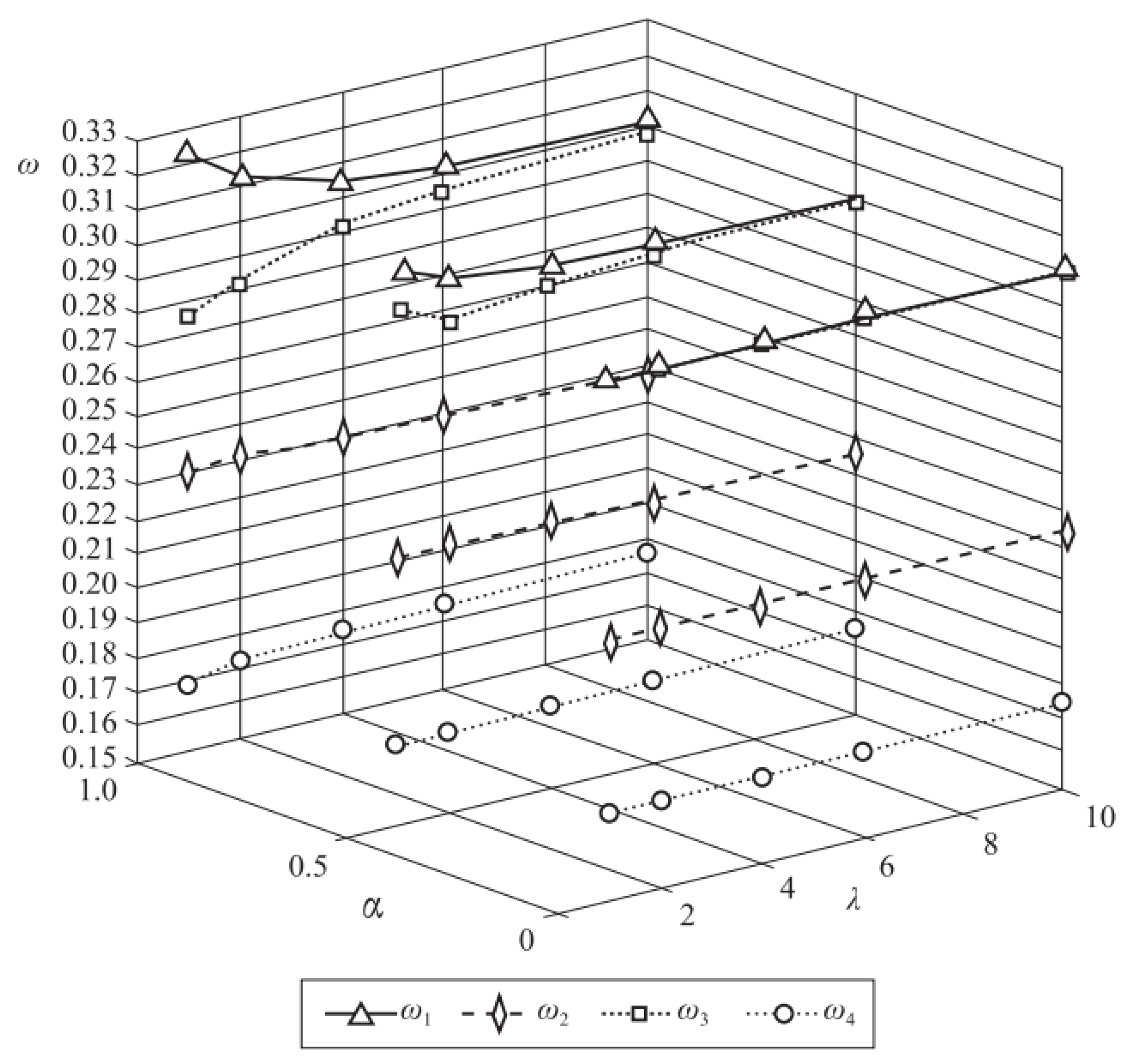
In this section, we further discuss how the changes in the values of the parameters influence the attribute weight and the optimal solution of the model.

7.1. The Effect of $\lambda$ on Attribute Weights

To observe the effect of parameter $\lambda$ on the attribute weight vector, we consider $\lambda$ = 2, 4, 6, 10, and $\alpha$= 0, 0.5, 1. The results are shown in

Table A1. The changes in the weight vector $\mathsf{\omega }=({\omega }_1,{\omega }_2,{\omega }_3,{\omega }_4)$.

$\mathit{\omega }$	$\mathit{\alpha }=0$	$\mathit{\alpha }=0.5$	$\mathit{\alpha }=1$
$\lambda =1$	(0.3000, 0.2250, 0.3000, 0.1750)	(0.3103, 0.2276, 0.2897, 0.1724)	(0.3231, 0.2308, 0.2769, 0.1692)
$\lambda =2$	(0.3000, 0.2250, 0.3000, 0.1750)	(0.3052, 0.2281, 0.2927, 0.1740)	(0.3129, 0.2321, 0.2825, 0.1725)
$\lambda =4$	(0.3000, 0.2250, 0.3000, 0.1750)	(0.3015, 0.2271, 0.2964, 0.1749)	(0.3043, 0.2301, 0.2910, 0.1746)
$\lambda =6$	(0.3000, 0.2250, 0.3000, 0.1750)	(0.3004, 0.2265, 0.2979, 0.1752)	(0.3012, 0.2287, 0.2947, 0.1754)
$\lambda =10$	(0.3000, 0.2250, 0.3000, 0.1750)	(0.2998, 0.2260, 0.2989, 0.1753)	(0.2997, 0.2273, 0.2972, 0.1758)

(in Appendix A), and the intuitive graphs are given in Figure 2.

According to Table A1 and Figure 2, we can observe that:

(1)

When $\alpha =0$, the weight vector, $\omega$, does not change with $\lambda$. When $\alpha =0.5$ or 1, ${\omega }_1$ and ${\omega }_2$ are decreasing, while ${\omega }_3$ and ${\omega }_4$ are increasing.

(2)

When $\lambda$ = 1, 2, 4, or 6, ${\omega }_1$ and ${\omega }_2$ are increasing, while ${\omega }_3$ and ${\omega }_4$ are decreasing. However, $\lambda$ = 10, ${\omega }_2$ and ${\omega }_4$ are increasing, while ${\omega }_1$ and ${\omega }_3$ are decreasing.

Based on the above findings, it indicates that different measurement coefficients $\lambda$ will influence the weight vector $\omega$, and the different buyers distance preference coefficients a will change the value of the weight vector $\omega$. The purchaser can select the parameters flexibly according to his own practical situation to determine the best attribute weight vector to evaluate the bids of the suppliers.

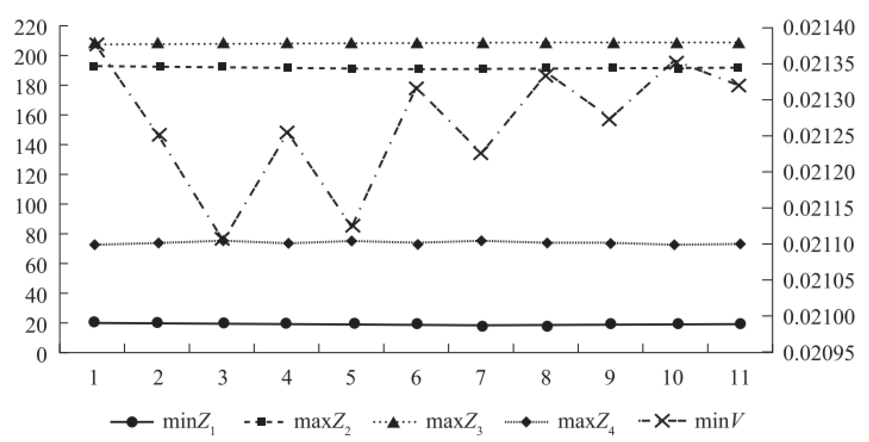
7.2. The Effect of the Changes in the Attribute Weight Vector, $\omega$, on the Optimal Solutions of Model-6

In this section, we observe the influence of the different attribute weight vectors on the optimal solutions of Model-3. The results are shown in

Table A2. The changes of the optimal results of Model-3, with respect to $\omega$.

$\mathit{\omega }$	Z1 (min)	Z2 (max)	Z3 (max)	Z4 (max)	V (min)	$({\mathit{q}}_1,{\mathit{q}}_2,{\mathit{q}}_3,{\mathit{q}}_4,{\mathit{q}}_5)$
(0.3000,0.2250, 0.3000,0.1750)—1	19.1408	193.4599	210.0669	73.7783	0.021379	(300,150,0,250,300)
(0.3103,0.2276, 0.2897, 0.1724)—2	19.2294	193.0836	209.864	74.7148	0.021254	(300,150,0,250,300)
(0.3231,0.2308, 0.2769, 0.1692)—3	19.3390	192.6191	209.6138	75.8717	0.021099	(300,150,0,250,300)
(0.3052,0.2281, 0.2927, 0.1740)—4	19.1877	193.1053	209.8394	74.6121	0.02125	(300,150,0,250,300)
(0.3129,0.2321, 0.2825, 0.1725)—5	19.2551	192.6351	209.5436	75.7261	0.021122	(300,150,0,250,300)
(0.3015,0.2271, 0.2964, 0.1749)—6	19.1541	193.2247	209.8943	74.2607	0.021316	(300,150,0,250,300)
(0.3043,0.2301, 0.2910, 0.1746)—7	19.1830	192.9330	209.7014	74.9805	0.021224	(300,150,0,250,300)
(0.3004,0.2265, 0.2979, 0.1752)—8	19.1408	193.4599	210.0669	73.7783	0.021379	(300,150,0,250,300)
(0.3012,0.2287, 0.2947, 0.1754)—9	19.1533	193.1038	209.8053	74.5716	0.021276	(300,150,0,250,300)
(0.2998,0.2260, 0.2989,0.1753)—10	19.1391	193.3708	209.9971	73.9711	0.021354	(300,150,0,250,300)
(0.2997,0.2273, 0.2972,0.1758)—11	19.1356	193.2537	209.9056	74.2253	0.021317	(300,150,0,250,300)

. Since the other four sub-objectives, MaxY₁, MinY₂, MinY₃, and MinY₄, are independent of the attribute weight vector 3, they are kept the same and not shown in Table A2 (in Appendix A). In order to see the changes of the results intuitively, Figure 3 is provided.

From Table A2 and Figure 3, we can observe: (1) The optimal values of the objective functions, Z₁, Z₂, Z₃, Z₄, vary with $\omega$ within a minimal range. (2) When $\omega$ = (0.3231, 0.2308, 0.2769, 0.1692) (i.e., $\alpha =1,\lambda =1$), the value of Z₄ (max) is biggest and the value of V (min) is smallest, indicating that the accuracy of the final decision can be improved when the decision-maker chooses the hamming distance from the distance preference. (3) The optimal decision scheme, i.e., the result for optimal selection and allocation is x = (1,1,0,1,1) and q = (300, 150, 0, 250, 300), and this also shows that the proposed method is robust in solving the OMSMARA problem.

7.3. The Effect of the Changes in the Sub-Objective Weight Vector, ($\beta ,\mu$), on the Optimal Solutions of Model-6

In this section, we observe the influence of different values of sub-objective weight vector ($\beta ,\mu$) on the optimal solutions of Model-3. The results are shown in

Table 8. The changes of the optimal solutions of Model-3 with respect to ($\beta ,\mu$).

$(\mathit{\beta },\mathit{\mu })$	$({\mathit{x}}_1,{\mathit{x}}_2,{\mathit{x}}_3,{\mathit{x}}_4,{\mathit{x}}_5)$	$({\mathit{q}}_1,{\mathit{q}}_2,{\mathit{q}}_3,{\mathit{q}}_4,{\mathit{q}}_5)$	V (min)
(1/8,1/8,1/8,1/8,1/8,1/8,1/8,1/8)	(1,1,0,1,1)	(300,150,0,250,300)	0.021254
(1/4,1/4,1/4,1/4,0,0,0,0)	(1,1,0,1,1)	(300,150,0,250,300)	0.042507
(0,0,0,0,1/4,1/4,1/4,1/4)	(1,0,1,1,1)	(300,0,150,250,300)	9.107 × 10−18
(0,1/2,1/2,0,0,0,0,0)	(1,1,0,1,1)	(300,150,0,250,300)	6.87 × 10−8
(0,0,0,0,0,1/2,1/2,0)	(1,1,0,1,1)	(300,150,0,250,300)	1.11 × 10−16
(1/6,2/6,2/6,1/6,0,0,0,0)	(1,1,0,1,1)	(300,150,0,250,300)	0.0283
(0,0,0,0,1/6,2/6,2/6,1/6)	(1,0,1,1,1)	(300,0,150,250,300)	9.02 × 10−17
(1/16,3/16,3/16,1/16,1/16,3/16,3/16,1/16)	(1,1,0,1,1)	(300,150,0,250,300)	0.0106

.

From Table 8, we can find that the first four sub-objectives of Model-3 are more sensitive to the change of target weight combinations, compared with the last four sub-objectives. The first four sub-objectives are equivalent to the corresponding first target value of Model-1, namely maximizing the total procurement value. This implies that, in an OMSMARA, the buyer is more inclined to maximize his procurement value. This is also in accordance with the actual procurement activities.

8. Comparative Analysis

In order to further demonstrate the effectiveness and reliability of the proposed decision framework, we compare the results obtained by the simple additive weighting (SAW) method and $\epsilon$-constraint method [48] for the same OMSMARA problem presented in this paper. For convenience and comparability, we use the same parameter setting (except ${\beta }_i$ and ${\mu }_i$), as shown in Table 2. Furthermore, the research contents and methods of this paper are compared with other relevant studies in the references, their similarities and differences are analyzed, and the important value and innovation of this study are pointed out.

8.1. The Comparison with the Results Obtained by the Simple Additive Weighting (SAW) Method

$$\mathrm{Min}{}_{}{}^{}\widehat{V}=w_1{F}_1+w_2{F}_2+w_3{F}_3+w_4{F}_4-{w^{\prime }}_1{U}_1-{w^{\prime }}_2{U}_2-{w^{\prime }}_3{U}_3-{w^{\prime }}_4{U}_4$$

(65)

$$\mathrm{s}.\mathrm{t}.{\displaystyle \sum _{i=1}^4(w_i+{w^{\prime }}_i})=1,{}_{}w{}_i,{w^{\prime }}_i\ge 0,{}_{}(55)–(63)$$

(66)

where $w_1,\cdots ,w_4,{w^{\prime }}_1,\cdots ,{w^{\prime }}_4$ are the weights of the sub-objectives. The results are shown in

Table 9. The results of the SAW method for solving the same OMSMARA problem.

$({\mathit{w}}_1,\cdots ,{\mathit{w}}_4,{{\mathit{w}}^{\prime }}_1,\cdots ,{{\mathit{w}}^{\prime }}_4)$	$({\mathit{Z}}_1,{\mathit{Z}}_2,{\mathit{Z}}_3,{\mathit{Z}}_4)$	$({\mathit{Y}}_1,{\mathit{Y}}_2,{\mathit{Y}}_3,{\mathit{Y}}_4)$	$({\mathit{q}}_1,{\mathit{q}}_2,{\mathit{q}}_3,{\mathit{q}}_4,{\mathit{q}}_5)$	$\widehat{\mathit{V}}(\mathit{m}\mathit{i}\mathit{n})$
(1/8,1/8,1/8,1/8, 1/8,1/8,1/8,1/8)	(22.498,193.084, 209.864,74.712)	(1080,6180, 6680,1080)	(300,150,0, 250,300)	−191.895
(1/4,1/4,1/4,1/4, 0, 0, 0, 0)	(22.498,193.084, 209.864,74.712)	(1080,6180, 6680,1080)	(300,150,0, 250,300)	−113.790
(0, 0, 0, 0, 1/4,1/4,1/4,1/4)	(20.257,181.904, 196.533,51.553)	(1080,6980, 7480,1080)	(300,250,300, 150,0)	−270
(0, 0, 0, 0, 0,1/2,1/2,0)	(22.501,191.380, 208.188,74.715)	(1080,6180, 6680,1080)	(300,0,150, 250,300)	0
(0,1/2,1/2,0, 0, 0, 0, 0)	(22.498,193.084, 209.864,74.712)	(1080,6180, 6680,1080)	(300,150,0, 250,300)	−201.474
(1/6,2/6,2/6,1/6, 0, 0, 0, 0)	(22.498,193.084, 209.864,74.712)	(1080,6180, 6680,1080)	(300,150,0, 250,300)	−143.018
(0, 0, 0, 0, 1/6,2/6,2/6,1/6)	(20.257,181.904, 196.533,51.553)	(1080,6980, 7480,1080)	(300,250,300, 150,0)	−180
(1/16,3/16,3/16,1/16, 1/16,3/16,3/16,1/16)	(22.498,193.084, 209.864,74.712)	(1080,6180, 6680,1080)	(300,150,0, 250,300)	−146.316

.

From Table 9, we can observe that by using the SAW method, there exist large fluctuations in the optimal allocation when the weights of the sub-objectives change. The main reason for the large fluctuation in the result of this method is that there is no exact method for the selection of weight in the SAW method, which has a certain randomness by the SAW method. That is to say, it is hard to set up a weight vector to get Pareto optimal solutions. Obviously, it will have a bad influence on the solution results of the procurement auction model in this paper. However, it is not difficult to find that, by using our proposed decision framework, the results of the solution are relatively stable, and most of the optimal allocations remain the same as shown in Table 7. This shows that our proposed decision framework is more robust for green supplier selection. In addition, by comparing the results in Table 7 and Table 9, we notice that our decision framework can obtain a higher procurement value, which is more favorable for the buyer. This further shows the advantage of our decision framework.

8.2. The Comparison with the Results Obtained by $\epsilon$-Constraint Method

$$\mathrm{Max}\overline{V}=Z_3$$

(67)

$$\mathrm{s}.\mathrm{t}.{}_{}Z{}_1\le {\epsilon }_1,Z_2\ge {\epsilon }_2,Z_4\ge {\epsilon }_4,Y_1\ge {{\epsilon }^{\prime }}_1,Y_2\le {{\epsilon }^{\prime }}_2,Y_3\le {{\epsilon }^{\prime }}_3,Y_4\le {{\epsilon }^{\prime }}_4,(55)–(63).$$

(68)

where Z₃ is seen as the main objective, and ${\epsilon }_i$ and ${{\epsilon }^{\prime }}_i$ are the new constraints. The results are shown in

Table 10. The results of the $\epsilon$-constraint method for solving the same OMSMARA problem.

$({\mathit{\epsilon }}_1,{\mathit{\epsilon }}_2,{\mathit{\epsilon }}_4,{{\mathit{\epsilon }}^{\prime }}_1,\cdots ,{{\mathit{\epsilon }}^{\prime }}_4)$	$({\mathit{Z}}_1,{\mathit{Z}}_2,{\mathit{Z}}_4)$	$({\mathit{Y}}_1,{\mathit{Y}}_2,{\mathit{Y}}_3,{\mathit{Y}}_4)$	$({\mathit{q}}_1,{\mathit{q}}_2,{\mathit{q}}_3,{\mathit{q}}_4,{\mathit{q}}_5)$	$\overline{\mathit{V}}={\mathit{V}}_3$
(19.2294,193.0836,74.7148 ,1080,6980,7480,1080)	(22.4983,193.0836,74.7122)	(1080,6180, 6680,1080)	(300,150,0, 250,300)	209.8640
(19.2294,193.0836,74, 1080,6980,7480,1080)	(22.4032,192.9976,74.0000)	(1080,6197, 6681,1080)	(281,169,0, 250,300)	209.6753
(19.2294,193.0836,74.7148,1080,6180,6680,1080)	(22.4983,193.0836,74.7148)	(1080,6180, 6680,1080)	(300,150,0, 250,300)	209.8639
(19.2294,193,74.7148, 1080,6180,6680,1080)	(22.5009,191.3797,74.7148)	(1080,6180, 6680,1080)	(300,0,150, 250,300)	208.1875
(19.2294,193.0836,75, 1080,6180,6680,1080)	(22.4983,193.0836,74.7122)	(1080,6180, 6680,1080)	(300,150,0, 250,300)	209.8639
(22,193,74.7148,1080, 6180,6680,1080)	(22.4983,193.0836,74.7122)	(1080,6180, 6680,1080)	(300,150,0, 250,300)	209.8640
(22,200,74.7148,1080, 6180,6680,1080)	(22.4983,193.0836,74.7122)	(1080,6180, 6680,1080)	(300,150,0, 250,300)	209.8640
(22,200,74.7148,1080, 6980,7480,1080)	(22.4983,193.0836,74.7122)	(1080,6180, 6680,1080)	(300,150,0, 250,300)	209.8640
(19.2294,193.0836,75, 1080,6980,7480,1080)	(22.4983,193.0836,74.7122)	(1080,6180, 6680,1080)	(300,150,0, 250,300)	209.8639
(19.2294,193.0836,74.7148,980,6180,6680,1080)	(22.5009,191.3797,74.7148)	(1080,6180, 6680,1080)	(300,0,150, 250,300)	208.1875
(19.2294,193.0836,74.7148,980,6980,7480,1080)	(22.4983,193.0836,74.7122)	(1080,6180, 6680,1080)	(300,0,150, 250,300)	209.8639

.

From Table 10, we can see that the optimal allocations obtained by the $\epsilon$-constraint method still have some fluctuations, although the fluctuations are smaller than that of using SAW method. Moreover, the optimal solutions are the same as those obtained from our proposed method, only when the ${\epsilon }_i$ and ${{\epsilon }^{\prime }}_i$ are taken equal to the optimal solutions obtained by our method as shown in Table 7. The main reason of above phenomenon is that the constraint methods generally retain only one objective function, while other objective functions are constrained by the set value, but the determination of this unique objective function needs careful selection, and the setting of constraint value is generally difficult. Different choices may lead to differences and changes in the solution results. However, our proposed decision-making framework effectively avoids the occurrence of the above problems, so the final result obtained becomes more stable. This indicates that our method is feasible, more robust, and reliable for auctioneers in OMSMARA practices.

8.3. The Comprehensive Comparison with the Other Related Literature

In this part, we comprehensively compare and analyze the relationship and difference between the research content and method of this paper, as well as the relevant existing literature research, which is carried out from the following aspects:

(1)

Compared with previous theoretical and applied research literatures on reverse auction and multi-attribute reverse auction, most of the previous literatures were developed from the perspective of game theory, such as [11,12,16,17,20,22,23,24,26,27,33], and less from the perspective of decision and optimization. In addition, the existing multi-attribute reverse auction literature from the perspective of decision and optimization, such as [13,14,19,25,28,30], did not consider the complex uncertain situation in the auction process, carried out analysis through simple multi-attribute decision method, or did not consider the real situation of multi-source procurement auction, and almost no online multi-sourcing multi-attribute reverse auction (OMSMARA) has been applied to the selection and order allocation of green suppliers. The most similar to this study in the literature [29], which studied the winner determination of risk-averse buyers in the multi-attribute reverse auction of clean energy equipment procurement with incomplete information and applied MARA to the winner determination of green suppliers of clean energy equipment. However, this paper fails to comprehensively consider the information uncertainty, the psychological influence of hesitation, and the application of fuzzy multi-objective optimization theory, and the proposed method cannot solve the problem of determining and quantitatively allocating multiple winning suppliers at the same time. To sum up, it can be seen that, compared with the previous application research on multi-attribute reverse auction, the research in this paper enriches theoretically and expands the application, which is helpful for promoting the promotion and development of auction theory and its application.

(2)

Compared with the previous literature on (green) supplier selection, the previous literature is more about the method of multi-attribute decision making or fuzzy multi-attribute decision making to select the right supplier. For example, [21,30,31,33,46,47] and some literatures model and solve the selection and order allocation problems of suppliers through common mathematical optimization methods, such as [32,34,35,36]. However, some of the above literature studies do not take into account the requirements of green attributes in green procurement, some rarely consider the application efficiency and practicability in real procurement, and almost no literature considers the application of OMSMARA technology to the selection and order allocation problem of green suppliers. The literature that are most similar to this study are [27] and [48]. The former introduces the multi- attribute auction mechanism into the universal supplier selection problem. However, it fails to take into account the possible uncertainties of bidding information in the process of procurement auction, the minds of decision-makers, and other aspects, as well as the requirements of green procurement multi-green attributes, which restricts the practicability and promotion of the research results. While the latter only applies MCDM and multi-objective optimization approach to solving the supplier selection and order allocation with green criteria, it neither considers the existence of uncertainty nor provides a more comprehensive and simple decision-making method to solve the problem of green supplier selection. However, the research in this paper makes up for the shortcomings of the above research. It not only considers the requirements of multi-green attributes in green procurement comprehensively, but also considers the various uncertainties faced by the auction parties. In addition, the decision method framework based on OMSMARA proposed by us can not only improve the value of procurement and reduce the cost of procurement. Moreover, it can effectively improve the efficiency of purchasing decision and the practicability of the decision-making method framework. The research contents of this paper not only enrich the theoretical system of decision-making method of green supplier selection, but also provide more practical decision-making method reference for more purchasing departments.

According to the above comparisons, it further shows the effectiveness, robustness, and practicability of our proposed decision framework for solving OMSMARA problem under various uncertain situations.

9. Conclusions

To seek the low-carbon and sustainable development of the economy and society, the green supply chain management of enterprises or governments becomes more and more important. How to quickly and efficiently select the suitable green supplier is the most basic and critical link in green supply chain management. So, this paper mainly studies how enterprises or government organizations can effectively select green suppliers in the procurement process. The OMSMARA, considering many non-price green attributes simultaneously online, is very suitable for selecting green suppliers, but the relevant research is scarce. Furthermore, in the existing literature about OMSMARA, it is rare to consider the impact of the various uncertainties of complex market environment and the hesitant psychology of the buyer (purchaser) simultaneously. Therefore, from the standpoint of the purchaser, a new decision framework of OMSMARA for green supplier selection under mixed uncertainty is proposed. The numerical example validated the rationality and applicability of our proposed framework, and the sensitivity analysis and comparative analysis verified the effectiveness and robustness of the proposed comprehensive decision framework for green supplier selection. Compared with the previous research, the method has a certain novelty, which can improve the efficiency of procurement decision and reduce the cost of procurement and decision-making risk.

The research content of this paper not only provides a new and effective way to solve the problem of green suppliers in procurement and can provide a decision-making reference for the relevant enterprises and government departments, but also can further expand the related application fields of OMSMARA. However, there are still many shortcomings in this study. For example, we assumed that there is only one decision-maker (the buyer) to provide the hesitant fuzzy decision matrix based on his own experience and judgment; however, there may be many decision-makers from different departments of a company or government to determine the weights for attributes jointly in reality. In addition, when introducing OMSMARA to solve the model construction of green supplier selection problem, in order to simplify the analysis, this paper made a lot of assumptions, which may not be consistent with the real auction situation, so the application scenario of the decision method proposed in this paper is limited. Furthermore, in the construction of the problem model in this paper, only the case of a single round of reverse auction was considered, instead of the possible case of multiple rounds of interactive negotiation in OMSMARA, which would also limit the applicability of the decision framework

Therefore, in combination with the shortcomings of the above research and references to the relevant literature [49,50,51,52], in future studies, we can make a further study from the following directions: (1) we can introduce the group decision-making method or consensus models to improve the precision of green supplier bidding evaluation attribute weight under mixed uncertainty. (2) we can also consider the robust optimization, machine learning, and stochastic optimization methods to deal with the complex uncertainties in green supplier selection problems in OMSMARA. (3) We can further relax the assumed constraints of the original problem model construction, constantly improve and enrich the existing theoretical model, and improve the applicability of the decision framework proposed in this paper.

References

1. Deng, Q.; Qin, Y.; Ahmad, N. Relationship between Environmental Pollution, Environmental Regulation and Resident Health in the Urban Agglomeration in the Middle Reaches of Yangtze River, China: Spatial Effect and Regulating Effect. Sustainability 2022, 14, 7801. [Google Scholar] [CrossRef]
2. Qu, S.; Xu, Y.; Ji, Y.; Feng, C.; Wei, J.; Jiang, S. Data-Driven Robust Data Envelopment Analysis for Evaluating the Carbon Emissions Efficiency of Provinces in China. Sustainability 2022, 14, 13318. [Google Scholar] [CrossRef]
3. Ehsan, E.; Zainab, K.; Muhammad, Z.T.; Zhang, H.; Xing, L. Extreme weather events risk to crop-production and the adaptation of innovative management strategies to mitigate the risk: A retrospective survey of rural Punjab, Pakistan. Technovation 2022, 117, 102255. [Google Scholar] [CrossRef]
4. Ehsan, E.; Zainab, K. Estimating smart energy inputs packages using hybrid optimisation technique to mitigate environmental emissions of commercial fish farms. Appl. Energ. 2022, 326, 119602. [Google Scholar] [CrossRef]
5. Abbas, A.; Zhao, C.; Waseem, M.; Ahmad, R. Analysis of Energy Input–Output of Farms and Assessment of Greenhouse Gas Emissions: A Case Study of Cotton Growers. Front. Environ. Sci. 2021, 9, 826838. [Google Scholar] [CrossRef]
6. Abbas, A.; Waseem, M.; Yang, M. An ensemble approach for assessment of energy efficiency of agriculture system in Pakistan. Energ. Effic. 2020, 13, 683–696. [Google Scholar] [CrossRef]
7. Maditati, D.R.; Munim, Z.H.; Schramm, H.-J.; Kummer, S. A review of green supply chain management: From bibliometric analysis to a conceptual framework and future research directions. Resour. Conserv. Recycl. 2018, 139, 150–162. [Google Scholar] [CrossRef]
8. Asha, L.N.; Dey, A.; Yodo, N.; Aragon, L.G. Optimization approaches for multiple conflicting objectives in sustainable green supply chain management. Sustainability 2022, 14, 12790. [Google Scholar] [CrossRef]
9. Li, C.; Liu, Q.; Li, Q.; Wang, H. Does Innovative Industrial Agglomeration Promote Environmentally-Friendly Development? Evidence from Chinese Prefecture-Level Cities. Sustainability 2022, 14, 13571. [Google Scholar] [CrossRef]
10. Zhu, M.; Yang, H.; Yuan, H.D. Talent internationalization and OFDI of China. Stud. in Sci. of Sci. 2019, 37, 245–253. (In Chinese) [Google Scholar] [CrossRef]
11. Teich, J.E.; Wallenius, H.; Wallenius, J.; Zaitsev, A. A multi-attribute e-auction mechanism for procurement: Theoretical foundations. Eur. J. Oper. Res. 2006, 175, 90–100. [Google Scholar] [CrossRef]
12. Pinker, E.J.; Seidmann, A.; Vakrat, Y. Managing online auctions: Current business and research issues. Manag. Sci. 2003, 49, 1457–1484. [Google Scholar] [CrossRef] [Green Version]
13. Cheng, C.-B. Reverse auction with buyer–supplier negotiation using bi-level distributed programming. Eur. J. Oper. Res. 2011, 211, 601–611. [Google Scholar] [CrossRef]
14. Huang, M.; Qian, X.; Fang, S.-C.; Wang, X. Winner determination for risk aversion buyers in multi-attribute reverse auction. Omega 2016, 59, 184–200. [Google Scholar] [CrossRef]
15. Long, P.; Teich, J.; Wallenius, H.; Wallenius, J. Multi-attribute online reverse auctions: Recent research trends. Eur. J. Oper. Res. 2015, 242, 1–9. [Google Scholar] [CrossRef]
16. Xu, S.X.; Huang, G.Q. Efficient Multi-Attribute Multi-Unit Auctions for B2B E-Commerce Logistics. Prod. Oper. Manag. 2016, 26, 292–304. [Google Scholar] [CrossRef]
17. Bichler, M.; Kalagnanam, J. Configurable offers and winner determination in multi-attribute auctions. Eur. J. Oper. Res. 2005, 160, 380–394. [Google Scholar] [CrossRef]
18. Zhang, J.; Xiang, J.; Cheng, T.E.; Hua, G.; Chen, C. An optimal efficient multi-attribute auction for transportation procurement with carriers having multi-unit supplies. Omega 2018, 83, 249–260. [Google Scholar] [CrossRef]
19. Liu, S.; Liu, C.; Hu, Q. Optimal procurement strategies by reverse auctions with stochastic demand. Econ. Model. 2013, 35, 430–435. [Google Scholar] [CrossRef]
20. Xu, J.; Feng, Y.; He, W. Procurement auctions with ex post cooperation between capacity constrained bidders. Eur. J. Oper. Res. 2017, 260, 1164–1174. [Google Scholar] [CrossRef]
21. Simić, D.; Kovačević, I.; Svirčević, V.; Simić, S. 50 years of fuzzy set theory and models for supplier assessment and selection: A literature review. J. Appl. Log. 2017, 24, 85–96. [Google Scholar] [CrossRef] [Green Version]
22. Che, Y.-K. Design Competition Through Multidimensional Auctions. RAND J. Econ. 1993, 24, 668. [Google Scholar] [CrossRef]
23. David, E.; Azoulay-Schwartz, R.; Kraus, S. Bidding in sealed-bid and English multi-attribute auctions. Decis. Support Syst. 2005, 42, 527–556. [Google Scholar] [CrossRef]
24. Bellosta, M.-J.; Kornman, S.; Vanderpooten, D. Preference-based English reverse auctions. Artif. Intell. 2011, 175, 1449–1467. [Google Scholar] [CrossRef] [Green Version]
25. Cheng, C.-B. Solving a sealed-bid reverse auction problem by multiple-criterion decision-making methods. Comput. Math. Appl. 2008, 56, 3261–3274. [Google Scholar] [CrossRef] [Green Version]
26. Hu, Y.; Wang, Y.; Li, Y.; Tong, X. An Incentive Mechanism in Mobile Crowdsourcing Based on Multi-Attribute Reverse Auctions. Sensors 2018, 18, 3453. [Google Scholar] [CrossRef] [PubMed] [Green Version]
27. Jain, V.; Panchal, G.B.; Kumar, S. Universal supplier selection via multi-dimensional auction mechanisms for two-way competition in oligopoly market of supply chain. Omega 2014, 47, 127–137. [Google Scholar] [CrossRef]
28. Singh, R.K.; Benyoucef, L. Fuzzy Logic and Interval Arithmetic-Based TOPSIS Method for Multicriteria Reverse Auctions. Serv. Sci. 2012, 4, 101–117. [Google Scholar] [CrossRef]
29. Qian, X.; Fang, S.C.; Huang, M.; Wang, X. Winner determination of loss-averse buyers with incomplete information in multi- attribute reverse auctions for clean energy device procurement. Energy 2019, 177, 276–292. [Google Scholar] [CrossRef]
30. Wang, S.; Qu, S.; Goh, M.; Wahab, M.I.M.; Zhou, H. Integrated Multi-stage Decision-Making for Winner Determination Problem in Online Multi-attribute Reverse Auctions Under Uncertainty. Int. J. Fuzzy Syst. 2019, 21, 2354–2372. [Google Scholar] [CrossRef]
31. Harridan, S.; Cheaitou, A. Supplier selection and order allocation with green criteria: An MCDM and multi-objective optimization approach. Comput. Oper. Res. 2017, 81, 282–304. [Google Scholar] [CrossRef]
32. Demirtas, E.A.; Ustun, O. An integrated multi-objective decision making process for supplier selection and order allocation. Omega 2005, 36, 76–90. [Google Scholar] [CrossRef]
33. Rao, C.; Xiao, X.; Goh, M.; Zheng, J.; Wen, J. Compound mechanism design of supplier selection based on multi-attribute auction and risk management of supply chain. Comput. Ind. Eng. 2017, 105, 63–75. [Google Scholar] [CrossRef]
34. Bohner, C.; Minner, S. Supplier selection under failure risk, quantity and business volume discounts. Comput. Indust. Eng. 2017, 104, 145–155. [Google Scholar] [CrossRef]
35. Cheraghalipour, A.; Farsad, S. A bi-objective sustainable supplier selection and order allocation considering quantity discounts under disruption risks: A case study in plastic industry. Comput. Ind. Eng. 2018, 118, 237–250. [Google Scholar] [CrossRef]
36. Assellaou, H.; Ouhbi, B.; Frikh, B. Multi-Objective Programming for Supplier Selection and Order Allocation under Disruption Risk and Demand, Quality, and Delay Time Uncertainties. Int. J. Bus. Anal. 2018, 5, 30–56. [Google Scholar] [CrossRef]
37. Torra, V. Hesitant fuzzy sets. Inter. J. Intell. Syst. 2010, 25, 529–539. [Google Scholar] [CrossRef]
38. Tong, X.; Yu, L. MADM based on distance and correlation coefficient measures with decision-maker preferences under a hesitant fuzzy environment. Soft Comput. 2015, 20, 4449–4461. [Google Scholar] [CrossRef]
39. Xu, Z.; Xia, M. On distance and correlation measures of hesitant fuzzy information. Int. J. Intell. Syst. 2011, 26, 410–425. [Google Scholar] [CrossRef]
40. Xu, Z.; Zhang, X. Hesitant fuzzy multi-attribute decision making based on TOPSIS with incomplete weight information. Knowl.-Based Syst. 2013, 52, 53–64. [Google Scholar] [CrossRef]
41. Zhang, X.; Xu, Z. The TODIM analysis approach based on novel measured functions under hesitant fuzzy environment. Knowl.-Based Syst. 2014, 61, 48–58. [Google Scholar] [CrossRef]
42. Li, J.; Wang, J.-Q.; Hu, J.-H. Consensus building for hesitant fuzzy preference relations with multiplicative consistency. Comput. Ind. Eng. 2019, 128, 387–400. [Google Scholar] [CrossRef]
43. Meng, F.; Chen, X. Correlation Coefficients of Hesitant Fuzzy Sets and Their Application Based on Fuzzy Measures. Cogn. Comput. 2015, 7, 445–463. [Google Scholar] [CrossRef]
44. Dong, J.-Y.; Wan, S.-P. A new trapezoidal fuzzy linear programming method considering the acceptance degree of fuzzy constraints violated. Knowl.-Based Syst. 2018, 148, 100–114. [Google Scholar] [CrossRef]
45. Wan, S.-P.; Dong, J.-Y. Possibility linear programming with trapezoidal fuzzy numbers. Appl. Math. Model. 2014, 38, 1660–1672. [Google Scholar] [CrossRef]
46. Chai, J.; Liu, J.N.; Ngai, E.W. Application of decision-making techniques in supplier selection: A systematic review of literature. Expert Syst. Appl. 2013, 40, 3872–3885. [Google Scholar] [CrossRef]
47. Qu, S.; Shu, L.; Yao, J. Optimal pricing and service level in supply chain considering misreport behavior and fairness concern. Comput. Ind. Eng. 2022, 174, 108759. [Google Scholar] [CrossRef]
48. Babbar, C.; Amin, S.H. A multi-objective mathematical model integrating environmental concerns for supplier selection and order allocation based on fuzzy QFD in beverages industry. Expert Syst. Appl. 2018, 92, 27–38. [Google Scholar] [CrossRef]
49. Qu, S.; Li, Y.; Ji, Y. The mixed integer robust maximum expert consensus models for large-scale GDM under uncertainty circumstances. Appl. Soft Comput. 2021, 107, 107369. [Google Scholar] [CrossRef]
50. Qu, S.; Wei, J.; Wang, Q.; Li, Y.; Jin, X.; Chaib, L. Robust minimum cost consensus models with various individual preference scenarios under unit adjustment cost uncertainty. Inform. Fusion 2023, 89, 510–526. [Google Scholar] [CrossRef]
51. Qu, S.; Xu, L.; Mangla, S.K.; Chan, F.T.S.; Zhu, J.; Arisian, S. Matchmaking in reward-based crowdfunding platforms: A hybrid machine learning approach. Int. J. Prod. Res. 2022, 60, 7551–7571. [Google Scholar] [CrossRef]
52. Ji, Y.; Li, H.; Zhang, H. Risk-Averse Two-Stage Stochastic Minimum Cost Consensus Models with Asymmetric Adjustment Cost. Group Decis. Negot. 2021, 31, 261–291. [Google Scholar] [CrossRef] [PubMed]
Figure 1. The flowchart of OMSMARA and the main content of the proposed decision framework.
Sustainability 14 16879 g001
Figure 2. The changing trend of the attribute weights.
Sustainability 14 16879 g002
Figure 3. The optimal values of the models vary with the parameter ω .
Sustainability 14 16879 g003