Abstract
It has become a hot topic in sustainable development to determine how to use data series to predict the trajectory of ecological footprints (EFs), precisely map biocapacity (BC), and effectively analyze regional sustainability. The sustainability of the ecological system in Gansu province must be investigated because the province is situated in western China and serves as a significant economic and transportation hub. We used the EF model to compute the per capita EF and BC of Gansu province from 2010 to 2020. We created a three-dimensional ecological footprint () model by incorporating the ecological footprint size () and ecological footprint depth () into the EF model and the of Gansu province from 2010 to 2020 was measured. The value was estimated using the gray GM (1, 1) prediction model in order to determine the sustainability condition of Gansu province during the next ten years. Finally, the risk of ecosystem loss in the province of Gansu was ultimately assessed using an ecological risk model (EVR). The results show that Gansu province’s per capita EF and BC displayed generally rising trends and the province is experiencing unsustainable development. The region’s projected future consumption of natural capital was estimated by the results, and the of Gansu province is expected to increase significantly in the future. These findings have a certain reference value for adjusting the industrial structure and utilizing resources in Gansu province. Furthermore, these findings will assist Gansu province in achieving sustainable development policy recommendations.
1. Introduction
The ecological environment is essential to human life and growth, and human behavior has a significant impact on the environment. Population growth and social and economic development have impacts on the planet’s ecosystem. Additionally, the problems (such as broad environmental deterioration, resource depletion, and the deteriorating relationship between man and nature) have increased. Consequently, sustainable development has become the consensus [1]. Researchers studied the ideas of social development and sustainable development, moving away from the idea of simple economic growth and toward the idea of integrated development of the economy, society, and the environment [2,3]. However, the scarcity of natural resources affects the quality of human activities [4]. This is a current research hotspot, i.e., how to handle the connection between natural assets, civilization, and economic growth under the constraints of ecological resources and the environment. Regional ecological sustainability is extremely significant to balance the connection between economic growth, social progress, and resource management [5]. Sustainable development goals call on all nations to take action in order to promote global prosperity through resource management, sustainable production and consumption, and environmental protection [6].
An ecological footprint (EF) was a term created by Rees et al. [7]. Biologically productive land (including land and water) is required to sustainably produce all resources needed by a population and to remove the waste generated is known as the ecological footprint [8,9,10]. The term biocapacity refers to the total amount of land and water that is genuinely available for biological production and that can be made available to people in a given amount of time, namely, the ability of natural resources to regenerate through time. The gap between the demand for natural ecosystem services from human economic systems and the carrying capacity of natural ecosystems was calculated and compared by Wackemagel et al. [11] to quantitatively assess the degree of sustainable resource use. The EF method offers a clear-cut theoretical framework for evaluating the sustainability of regional development [12]. For example, at the global level, Andreína et al. [13] analyzed and researched BC and EF, and predicted and analyzed biodiversity and the environmental footprint behaviors of five continents (up to the year 2030) through a neural network. At the national level, according to the national average output from 1989 to 2018, Sobhani et al. [14] examined the semi-arid climate zone of Iran to determine the sustainability of resource use and the pressure that human activities place on natural capital. Kovacs Zoltan et al. [15] analyzed the environmental sustainability of Hungarian urbanization and the long-term changes in environmental footprints and biological capacity. At the regional level, Zhang et al. [16] built a framework for evaluating Panzhihua City’s sustainable development from 2000 to 2020 based on EF; they developed an EF model using the provincial hectare as the unit. The city’s capacity for sustainable development was then thoroughly assessed using a collection of ecological indices, including EPI, EFG, ESI, and ECI. Sonia and Samir [17] used the bottom-up model based on component EF technology to determine the demand of Algiers fishing port for fishery resources. The classic EF calculation approach was enhanced by Xie et al. [18], who also created the port energy EF model and researched the ecological state of port logistics from 2009 to 2018. Additionally, using the EF model, Yang et al. [19] and Li et al. [20] assessed regional sustainable development.
To create the model, Niccolucci added and to the EF model [21,22]. The model was introduced to China by Fang et al. [23,24], who also improved it to address the offset issue with various land-use patterns. The capital inflow utilization ratio and the capital stream’s quota were devised to assess how natural capital was used in 11 countries. While energy use and economic status significantly impact the footprint, the model better captures regional growth. Based on an optimized and the human development index at the metropolitan scale, Long et al. [25] developed a model for evaluating ecological well-being performance and the efficacy of local sustainable development. The revised model was used by Chen et al. [1] to thoroughly assess the ecological security status in Henan Province from 2007 to 2016. According to the report, Henan province’s capital flow is in an unsustainable stage of development. Deng et al. [26] assessed the ecological efficiency of Hunan Province based on the model. Their research provides a scientific basis for other provinces to establish sustainable development strategies for ecological civilization.
When revealing and predicting the economy, the EF prediction is crucial to forecast the value of urban ecological environments, assess their state of development, and offer acceptable and workable policy recommendations to regional decision-makers for sustainable development [13]. The question of how to correctly forecast the evolution of EF values has received a lot of attention, and numerous techniques have been employed to model future EF. Deep neural networks were utilized by Andreína et al. [13] to adapt data to the global footprint network and make predictions. In order to calculate and simulate the EF value of Suzhou from 1999 to 2018, Yao et al. [27] used the ARIMA model and the GM (1, 1) model. They also examined the city’s current state of ecological sustainability. The EF of Shandong province from 2018 to 2030 was predicted by Li et al. [28] using the BPNN technique, along with whether or not future economic policies would lessen or accelerate ecological degradation. Su et al. [29]’s predictions for 2020 and 2025 regarding the per capita water EF were made using the quadratic exponential smoothing technique. The Gray prediction was utilized by Peng et al. [30,31] to predict the EF.
Ecological risk assessment is a new technical means and method used to assess and manage various ecological risk probability problems in the ecological environment [32]. Numerous experts have begun to perform numerous ecological environmental studies to slow down the ecological environment’s destruction and enhance the living conditions of humans. Researchers have created and enhanced the content, breadth, methodologies, and models of ecological risk assessment after more than 20 years of development. Researchers from all over the world have even started utilizing the theories and methods of ecological risk assessment to completely evaluate the numerous hazards faced by ecological systems due to the theory’s rapid development and the rise in the popularity of ecological problems. For instance, the landscape’s ecological risk index was developed by Liu et al. [33,34,35] to direct the sustainable use of land resources. The ecotoxicity of heavy metals in sediment columns was evaluated using the following metrics by Nimmi et al. [36,37]: pollution degree, organic pollution index, contributing factors, site accumulation index, potential ecological indicator, toxicity unit, and toxicity risk index. Liu [38] employed the VAR method of financial risk analysis market portfolio to perform a risk analysis of the value of ecosystem services, and he designated the EVR (ecological value at risk) model.
The social economy of northwest China cannot grow sustainably owing to the region’s difficult environmental circumstances, precarious ecological status, frequent human activities, and numerous environmental issues [39]. A substantial commercial and transportation hub, specifically in the province of Gansu, contributes significantly to the social and economic growth of the northwest region and even the entire country. The social and economic development of Gansu province is currently being hampered by ecological issues, which have grown to be the biggest issues [40,41]. As a result, it is imperative to research the ecosystem of Gansu province to support its sustainable growth. Based on this, we focused on the province of Gansu, calculated its EF value and value from 2010 to 2020, and used the GM (1, 1) model to predict its value from 2020 to 2030 in order to assess its level of sustainable development. For the risk analysis of the value of ecosystem services, we use the VAR method of the financial risk analysis market portfolio [42]. To evaluate the ecosystem risk in Gansu Province from 2010 to 2020, an ecosystem risk model was developed. It offers a fresh concept for the ecological economy’s long-term growth in Gansu province.
2. Materials and Methods
2.1. Study Area
In the high and middle reaches of the Yellow River, the western Chinese province of Gansu is located between poles 32°11′–42°57′ N and 92°13′–108°46′ E [40] (Figure 1). The overall area of Gansu province, which makes up 4.72% of China’s total area, is 454,430 square kilometers, with an east–west length of 1659 km and a north–south breadth of 530 km. The climate diversity, biological diversity, and landform diversity are highly apparent because the east and west are long and narrow. The Yellow River, the Yangtze River, three inland river basins, and nine river systems are the principal sources of water in Gansu province. Grassland and woodland make up most of the province’s land types, followed by cultivated land. As of the end of 2018, 119 different types of minerals have been found there. The province receives 400 mm of rain on average each year, and the average annual temperature ranges from 4 to 15 °C, depending on the location [43]. There is a lot of sunshine, and the temperature swings dramatically. The province’s primary economic sectors, including farming, forestry, industrial, animal rearing, tourism, and the ecological environment, greatly impact the provincial economy.
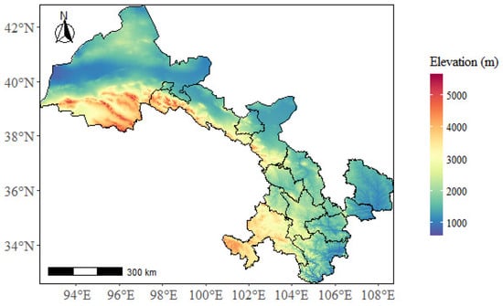
Figure 1.
Location of the study area.
2.2. Data Sources
This study opted to analyze the changes in the ecological environment in Gansu province from 2010 to 2020 based on the availability of the data itself in order to correctly portray the features of sustainable changes in the ecological environment of Gansu Province. The six categories of land use types in the basin are fossil energy, building land, cultivated area, grassland, forest land, and water area. These categories are based on the “Land Use Status Classification” standard established by the Ministry of Land and Resources. Table 1 displays the biological productivity accounts for the various types of land in Gansu province. Additionally, research on energy consumption primarily concentrates on coal, gasoline, natural gas, electricity, and other fuels. The two resource datasets mentioned above come from the Gansu Statistical Yearbook for 2010–2020.

Table 1.
Biological productivity accounts for various land types in Gansu Province.
The degrees of productivity of the six biologically productive lands varied in different places, thus the data were translated to areas with the same environmental value by multiplying the land areas of the six diverse productivity levels by a balance factor. This study is based on the “Equivalence factor” of China’s EF, which Wackernagel presented in the “National Footprint and Biocapacity Accounts” report in 1997; the difference in supply capacity is a critical criterion. This study corresponds to the actual condition of Gansu province. We calculate the “Production Factor” for each year by combining the annual different productivity (average annual output) of Gansu province with the global average productivity statistics on biological resources published by the United Nations Food and Agriculture Organization in 1993 (see Table 2).
Table 2.
Equivalence factor and production factor of biologically produced land.
Additionally, according to a report by the World Commission on Environment and Development (WCED) [44,45], about 12.0% of the land is used for biodiversity protection. Therefore, 12.0% of the land in this study’s calculation of BC was subtracted as ecological protection land for the region, leaving the remaining land to contain biological resources [19]. The boundary data of Gansu province were obtained from the Aliyun platform (https://datav.aliyun.com, accessed on 14 May 2022).
2.3. Research Methods
The EF, which includes the volume of total resource consumption in a given area and the scale of resource availability, is the total amount of land resources utilized by human activities. It also exposes the ecological threshold for sustained human life [5]. It consists of six different types of land resources: fossil energy, building land, cultivated area, grassland, woodland, and water area. The six lands produce differently on average. For the purpose of comparing the calculations, an equilibrium factor was multiplied by each land type, and EF was then computed using the weight of the biologically productive land area. This is the calculation’s formula.
where ef is the per capita ecological footprint (hm2/cap); is the equivalence factor of Gansu province; i is the consumption of ith types; j is the land types; is the per capita consumption of ith commodities; is the global average output of the ith projects; N is the total population of the region (cap).
The total amount of productive land in an area that can supply resources and energy for consumption by locals is known as biocapacity (BC). The unit production of the six land types varies depending on each region’s resources and land productivity. The actual acreages of specific types of biological production land in various countries and regions were compared using the standards and production features of various forms of biological production land. The formula below is used to determine BC.
where bc is the per capita biocapacity (hm2/cap); is the per capita biological production area of the jth project; is the production factor.
Ecological carrying capacity (ECC) is a measure of the effective use of natural resources by a population in a study area. When EF decreases BC and the calculation result is negative, it is called ecological reserve (ER), indicating that the resource demand of the area is sustainable. When EF minus BC is positive, it is called ecological deficit (ED). An ecological deficit is a situation in which an area’s available resources exceed its ecological capacity. Therefore, this development is not sustainable. The formula is described as,
Numerous academics have researched the model. and are two fundamental indicators employed in the model to represent the buildup of the ecological overdraft over time. While measures the human occupancy of yearly natural capital income, measures the depletion of natural capital stock.
With the aid of , we can assess the sustainability of current human activities and development trends in relation to the limitations of renewable resources and ecological services without depleting natural capital stocks. We can also identify which biological components are overloaded in the study area.
2.4. The Gray GM (1, 1) Model Introduced
The term “gray system” was first used in an academic study by Professor Deng in the 1980s, when the gray system theory was initially proposed [46]. A system with partial information, where some information is unknown, is referred to as a “gray system”. In order to achieve the quantitative prediction of the system’s future changes, GM (1, 1), the fundamental model of the gray forecasting theory, essentially fits the original data series exponentially using the least squares approach after starting with a quadratic function [5]. Less historical data and low sequence integrity and reliability are issues that the model is better able to address. It can also generate erroneous original data to produce generated sequences with high regularity, and the operation is straightforward and simple to verify.
- 1.
- Sequence generation by accumulation;The accumulation generation number 1-AGO serves as a placeholder for a single operation represents the from 2010 to 2020, and creates the cumulative sequence.
- 2.
- Model establishment and solution;This series is used to generate the prediction model, which is based on a first-order differential equation with a single variable and is known as the GM (1, 1) model. The gray differential equation and the corresponding whitening differential equation are established. By the least square method, we find the estimate of u that minimizes . The GM (1, 1) model’s time-response function was obtained.
- 3.
- Calculation of the residual error and the relative error.where is the residual error and is the relative error.
2.5. Model of Ecological Value at Risk
The term “ecological risk” refers to the risk to which the ecosystem and its components are exposed [47]. It describes the potential effects of unforeseen accidents or disasters on the ecosystem and its constituents in a specific location. These outcome effects may damage the ecosystem’s structure and function, putting its safety and well-being in jeopardy.
2.5.1. Risk Calculation Method
Expectation and standard deviation are two different types of risk indicators used in ecosystem risk assessment [38,48]. Expectation primarily reflects a central tendency of risks; the higher the expectation value, the greater the overall risk. Standard deviation reveals the level of dispersion of risk or deviation from the indicator.
Expected value:
where are the discrete risk variable and its corresponding probability.
Standard deviation:
2.5.2. Ecological Value at Risk Model
The ecological value at risk (EVR) of the region was calculated as part of the regional ecosystem risk management model, which is a risk assessment model [38]. In general, we define it as the worst-case loss of a certain type of ecological index or its comprehensive index is predicted to occur at a specific point in the future, i.e., the maximum potential loss, in a normal ecological environment and at a specific confidence level. It is simple for ecosystem managers to monitor, operate, and control by determining the amount of energy exposed to risk in the regional ecosystem and comparing the numerical numbers.
We define as the total EF of resource i consumed in the n year in the region, is the growth rate of the total ecological consumption of the i resource in the n year in the region, is the maximum value where the growth rate of the EF of the i resource in the year is lower than the initial expected value under a certain confidence level where is the initial expected value and the standard deviation is
The mathematical description is:
It means that the growth rate of the ecosystem EF of the i resource in the region in year may be which will not be lower than the initial expectation by .
Due to
Further, we obtain the following formula.
It means that in the future, the maximum loss of the ecosystem EF rate of the i resource in the region with in the year is
2.5.3. EVR Model Calculation Method
The footprint of the ecosystem is assumed to be approximately normally distributed. Because of the existence theorem: if a random variable then To do this, we first normalize the distribution of the ecological footprint, namely:
Transform (11) into
when the confidence interval is given, by looking up the standard normal distribution quantile table, the quantile can be obtained, and the value can be solved.
2.5.4. Model Evaluation
In the process described above, we researched the risk of loss and developed a risk model for to assess the risk of in Gansu province from 2010 to 2020. The relevant recommendations are provided in the conclusion to lessen the risk of losing the ecosystem’s economic value in this area.
3. Results
3.1. Evaluation of the EF and BC in Gansu Province
3.1.1. Calculation of the EF and BC in Gansu Province in 2020
Both biological resources and fossil energy resources are taken into account while calculating EF. The biological resources vary according to location. Crop, animal, and aquatic products are how we categorize the utilization of biological resources [49]. A total of 15 biological resources were chosen from the total number available, including grains, vegetables, fruits, meat, milk, and aquatic products. To obtain the appropriate per capita EF, we translate the global average production into biological resources. Table 3 present the findings.
Table 3.
Biological resources in the per capita EF of Gansu province in 2020.
Coal, gasoline, natural gas, and electricity were our four basic choices for fossil fuels. The world average EF conversion factor is converted to the fossil land area, other energy consumption types are converted to fossil energy, and electricity is converted to the building land area. Table 4 lists the outcomes. The findings indicate that in 2020, Gansu province’s per capita fossil energy use was 0.0805 hm2/cap, while its per capita coal usage was 0.0696 hm2/cap, making up 86.46% of the total per capita fossil energy use area. These results suggest that the coal industry still accounts for the majority of energy consumption in Gansu province, despite the fact that coke significantly pollutes the air and environment and that the province’s energy consumption structure is inefficient.
Table 4.
Fossil energy resource accounts in the per capita EF of Gansu province in 2020.
In 2020, the biological production area in Gansu province was used to compute and compare per capita EF and BC. Grassland, with a per capita EF of 1.1736 hm2/cap, was the most significant EF in Gansu province in 2020, followed by the cultivated area and fossil energy (Table 5). The cultivated area, with a per capita BC of 1.9162 hm2/cap, is the largest in a similar manner to the Grassland. In Gansu province, per capita EF in 2020 was 3.2039 hm2/cap, whereas per capita BC was just 2.4457 hm2/cap. The per capita available BC was 2.1522 hm2/cap, and the per capita ECC was 1.0517 hm2/cap after 12% of biodiversity protection reserves were subtracted from the per capita BC. It demonstrates that the region’s supply of land resources falls well short of the demand, and the ecological system is in an unsustainable condition.
Table 5.
Per capita EF and BC of Gansu province in 2020.
The scarcity of fossil energy land is the most significant among the many land use types, followed by the shortage of grassland. This is strongly tied to Gansu province’s lack of development. Energy is used extensively in industrial production as the local economy grows. By using fossil fuels, the region’s water, land, and other resources will become more polluted, its economic growth rate will slow, and its ability to develop sustainably will be impacted. Building land should also be taken into consideration as it is also becoming saturated (Figure 2).
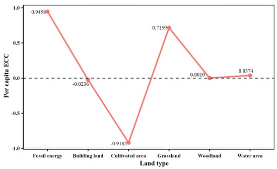
Figure 2.
Per capita ECC of Gansu province in 2020.
3.1.2. Dynamic Changes in the per Capita EF and BC in Gansu Province between 2010 and 2020
The per capita EF and BC of Gansu province were calculated using the same methods from 2010 to 2020. The BC was given the value of BC × 0.88 since 12% of the area should be reserved for conserving biodiversity after deduction. The variation trends of per capita EF and BC in Gansu province from 2010 to 2020 are depicted in Figure 3 and Figure 4. We discovered that the variations in per capita EF and BC trends tended to follow similar patterns: they increased from 2010 to 2015, decreased gradually from 2015 to 2019, and then significantly increased from 2019 to 2020. At the same time, we can see that the annual change trends of the six different land types are not particularly clear.
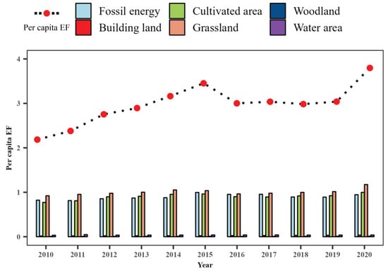
Figure 3.
The development trend of the per capita EF in Gansu province from 2010 to 2020.
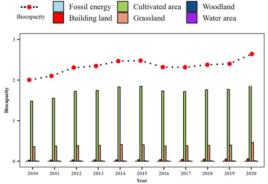
Figure 4.
The development trend of the BC in Gansu province from 2010 to 2020.
Figure 5 shows that the per capita EF in the fraction of grassland is the highest; fossil energy and cultivated area are comparable. In BC, the cultivated area is the largest, followed by grassland, while fossil energy accounted for 0. The cultivated area per capita EF is less than BC, indicating the area of Gansu province is in a surplus. Grassland per capita EF is greater than BC, illustrating that the grassland area of Gansu province is in a state of deficit. It is important to note that fossil energy is experiencing a deficit. Additionally, we discovered that there is relatively little variance in the annual land area of different forms of biological production.
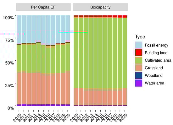
Figure 5.
The proportion of per capita EF and BC land types in Gansu province from 2010 to 2020.
3.1.3. Dynamic Evolution of the in Gansu Province from 2010 to 2020
Table 6 demonstrates that in Gansu province, the climbed from 1.6514 hm2 in 2010 to 2.0240 hm2 in 2015, then fell to 1.8981 hm2 in 2016 before rising to 2.1522 hm2 in 2010. With variations over time, Gansu’s climbed from 2.5721 hm2 in 2010 to 3.0689 hm2 in 2015 and then declined to 2.8921 hm2 in 2016, finally reaching 3.2039 hm2, which is consistent with variations in the trends of per capita EF. The ecological and economic developments of Gansu province were in deficits from 2010 to 2020, as evidenced by the fact that the has always been larger than 1 and the EF always exceeds the BC.
Table 6.
in Gansu province from 2010 to 2020.
According to Figure 6, the per capita ECC in Gansu province from 2010 to 2012 showed a steady decline, i.e., the unsustainable development status of Gansu province was eased. However, per capita ECC in Gansu province increased gradually between 2012 and 2015, indicating that with the change in the economy and the improvement in living standards, as the consumption of biological resources and fossil energy continues to increase, the sustainability of Gansu province will decline year by year and the contradiction between social and economic development and environmental resource management will become more obvious. The Gansu province’s per capita ECC fell between 2015 and 2018, indicating that the province’s resource utilization rate is increasing but can still be improved. Per capita ECC in Gansu province rose sharply from 2018 to 2020, and the state of unsustainable development still needs more attention.
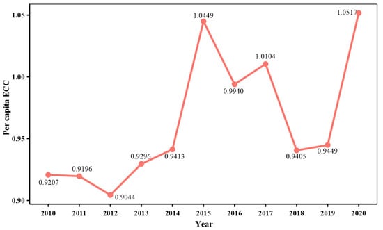
Figure 6.
Per capita ECC in Gansu province from 2010 to 2020.
3.2. Prediction by GM (1, 1) Model
The analysis in 3.1.3 informs us that the of Gansu province from 2010 to 2020 displayed a fluctuating rising tendency during the course of the study period. The GM (1, 1) model is capable of simulating it. The GM (1, 1) model was developed using the data series of the values. Following the execution of the software, the model precision and the fitting values could be acquired (Table 7). Figure 7 shows a visualization of the GM (1, 1) model’s simulation performance. In the left ordinate of Figure 7, the relative error () is between −0.0426% and 0.0575%, while the residual error () is between −0.1239 and 0.1764.
Table 7.
The estimated in Gansu province from 2010 to 2020.
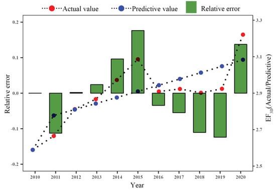
Figure 7.
estimated erformance of the GM (1, 1) model.
Gray system modeling is a technique for identifying the features of complex data and creating precise simulation models [50,51]. It can forecast nonlinear data sequence events. The value of this region’s EF is dynamic, complicated, and nonlinear, and a variety of socioeconomic factors may influence it. According to the above-mentioned fitting results, the gray model is capable of understanding the nonlinear relationship between the series, and the GM (1, 1) model’s simulation performance is precise (Figure 7).
However, the approximation model invariably results in certain simulation mistakes (relative errors in Figure 7). Prior to 2012, when the relative error was minor, the value was relatively low and the model overestimated the actual . From 2013 to 2015, the model somewhat underestimated the value of the , with a reasonably big relative error in 2015. With a significant relative inaccuracy, the model once more overestimated this parameter from 2016 to 2019. The value of the after 2020 was marginally underestimated by the model. The relative inaccuracy fluctuates generally, and the changing trend of the value in Gansu province is strongly tied to the reality of the situation.
The forecast is a projection of Gansu province’s future use of natural resources. According to forecasts, the province’s will increase to 3.4457 by 2030, or 1.34 times what it was in 2010 (Table 8). Future forecasts predict a steady rise in the of Gansu province. This implies that Gansu province’s ECC will keep growing and the region is already undergoing unsustainable regional development. Regarding sustainability, Gansu province will encounter formidable obstacles. To achieve sustainable urban growth, local governments should create relevant regional strategic plans with a focus on increasing energy efficiency, developing high-tech businesses, gradually modifying the industrial structure, and reducing the percentage of the industry. By raising the GDP share of the tertiary sector, creating more environmentally friendly products, etc., the city can reduce its use of natural resources and return to the path of sustainable growth.
Table 8.
The prediction of in Gansu province from 2021 to 2030.
3.3. Ecological Risk Assessment in Gansu Province
The of Gansu province is assessed for risk from 2010 to 2020 using an risk model. The process is broken down into four steps: organizing the data, estimating the expectation and standard deviation, estimating the EVR value, and figuring out the maximum loss.
3.3.1. Organize Data
We verify the pertinent ecological data for Gansu province from 2010 to 2020, then use the footprint model to determine the 11-year EF and .
3.3.2. Calculate the Expectation and Standard Deviation
The expectation of the growth rate of the in Gansu province in 2021, as well as the standard deviation, are displayed in Table; they are based on the definition and algorithm of the EVR model (Table 9).
Table 9.
Growth rate of and its expectation and standard deviation.
As shown in the above table, the expected growth rate of in Gansu province in the recent 11 years (2010–2020) is 2.2982%, and the standard deviation is 4.1885%.
3.3.3. Calculate the Value of EVR
In this paper, seven confidence levels of 50%, 80.00%, 90.00%, 95.00%, 97.50%, 99.00%, and 99.90% were selected, and the EVR values of the growth rate at different confidence levels were calculated using the quantile table of standard normal distribution (see Table 10).
Table 10.
EVR values of growth rates at different confidence levels.
Table 10 shows that, at the 99.90% confidence level, the EVR value of the growth rate in Gansu province in the recent 11 years (2010–2020) is 12.9425%. This indicates that the growth rate of in Gansu province is 99.90%, which is likely to be 12.9425% lower than the expected growth rate of 2.2982 ha/cap.
3.3.4. Maximum Loss
By calculating the EVR value of at the 99.90% confidence level, the maximum loss table of from 2010 to 2021 was calculated according to the EVR model (See Table 11).
Table 11.
Maximum loss of at the 99.90% confidence level.
According to Table 11, the maximum loss value of in Gansu province in the recent 11 years (2010–2020) was 0.3410.
4. Discussion
4.1. Comparison and Discussion of Results
Based on the aforementioned calculations and analysis of EF, BC, and in the Gansu province from 2010 to 2020, it is clear that, out of all the different types of land use, the scarcity of fossil energy land is the most important. The coal industry continues to be responsible for the vast majority of energy consumption in the province. Energy use in industrial output has increased significantly with the growth of the local economy. By burning fossil fuels, the region’s water, land, and other resources will become more badly polluted, the rate of economic growth will drop, and it will be more difficult to achieve sustainable development. This conclusion is in line with the findings in [40], which calculated the rate of change and scissors difference of the per capita EF and BC time series in Gansu Province between 1991 and 2003. According to the findings, fossil fuel usage has almost doubled in recent years. In Gansu province, the carrying capacity of the ecological environment has decreased due to overuse and depletion of natural resources. We can observe consistency between the outcomes produced by various techniques. We can also draw the same conclusion from [1,41].
We discovered that the grassland area in Gansu province is deficient, and one of the potential causes of this finding may be due to overgrazing in the pastoral districts of Gansu province. The government ought to encourage herdsmen to choose the appropriate number of animals to graze based on the size of the grassland [52]. Herdsmen might receive incentives and subsidies from the government if they minimize the quantity of grazing. This will help us to address the issue of overgrazing, increase the yield and coverage of grassland vegetation, and increase the carrying capacity of grassland [53]. In addition, the footprint of building land in Gansu province is approaching its carrying capacity due to population increase, faster urbanization, and large-scale urban construction. In the medium term, changing the method of production and hastening structural adjustment remain challenging tasks. From 2010 to 2020, the ecological economy’s growth in Gansu province fell short of expectations. Future trends indicate that in Gansu province will increase steadily. This means that the ecological deficit of Gansu province will continue to grow, and the region is already in unsustainable regional development. In terms of sustainable development, Gansu province will face huge obstacles.
4.2. Policy Implication
Based on the aforementioned research findings, the following suggestions are given for the sustainable development of Gansu Province in order to improve regional sustainability. (1) Slow down EF’s rate of growth by controlling the population. Change the unreasonably high human consumption mode and lower EF on the assumption that consumption will not be reduced. (2) We will actively promote the development of low-carbon circular economy industries, enhance resource utilization effectiveness, and cut back on the use of fossil fuels. Additionally, for companies that consume a lot of energy, emphasis should be placed on industrial structural transformation, energy conservation, emissions reductions, and assisting Gansu Province’s sustainable development. (3) To build a healthy environment, we will continue to step up the implementation of ecological projects, such as converting cropland back to forests and grasslands and combining agriculture and animal husbandry. (4) Change the industrial structure and utilize various land resources in a balanced manner. It is possible to implement scientific and logical resource allocations by making the necessary adjustments to the industrial structure. (5) By advancing science and technology, we can boost productivity, raise biocapacity, close the gap between EF and BC, and finally put Gansu province back on the path to sustainable development. (6) Boost ecological awareness while cutting down on resource waste. The government ought to prioritize environmental preservation initiatives, enact stringent laws and regulations, and raise public knowledge of energy conservation.
4.3. Limitations and Prospects of the Study
This study still has limitations. Only 11 years (2010–2020) of ecological footprint and biocapacity calculations have been made to examine the state of sustainable development in Gansu province, which may cause certain issues with the consistency and reliability of the model’s calculation results. The outcomes differ when using different equivalence and production factors. The ecological footprint as a tool for measuring sustainability may have limited application due to different results. Future ecological footprint research must continue to enhance ecological footprint accounting. The short-term future can only be assessed using the GM (1, 1) prediction model, while the long-term future cannot be predicted. Therefore, it will be crucial to enhance the EF model and combine several prediction models in future studies in order to accomplish a more thorough evaluation of various regions. These initiatives may offer more practical means of enhancing the equilibrium between ecological economics and sustainable development.
5. Conclusions
The EF model was utilized in this study to examine how sustainable use has changed over time in Gansu province. First, using the EF method, we calculated the per capita EF and BC of Gansu province from 2010 to 2020. We discovered that Gansu province’s per capita EF and BC displayed a generally rising trend. Second, we determined the of Gansu province from 2010 to 2020 using the model. Our research revealed that Gansu province is experiencing unsustainable development because was always larger than 1 over the study period, indicating that EF is always greater than BC. Then, the GM (1, 1) model was presented in order to simulate and forecast the of the province of Gansu. Through a test of model correctness, it was established that the GM (1, 1) model was appropriate for accurate data series simulation and short-term value forecasting in Gansu province. Our projected future consumption of natural capital was estimated by the results. The of Gansu province is expected to increase significantly in the future and will be 1.34 times higher in 2030 than it was in 2010. As a result, Gansu province’s economy will continue expanding, and the region is currently in an unsustainable stage of regional development. Finally, the values of Gansu province were utilized as historical data to estimate the risks faced by the ecological system in Gansu province from 2010 to 2020 using the ecological risk EVR model. The findings revealed the following: using a 99.90% confidence level as an example, we found that the growth rate of in Gansu province from 2010 to 2020 had an EVR value of 12.9425%, and it was 99.90% likely to not be lower than the initial assumption of 2.2982%. Thus, the annual rate of the ecosystem in this area is 99.90% likely to undergo a maximum loss of 0.3410 in the future.
On the basis of the data shown above, pertinent suggestions are given for the sustainable ecological and economic development of Gansu Province. The occupation of flow resources is growing as a result of the province’s development, and the cumulative impact of stock resource use is becoming more obvious as shown by the increasing footprint of fossil fuels and arable land per person. Thus, the region should develop a sensible consumption pattern and advance the development of ecological civilization under the presumption of environmental protection. In addition to identifying regional goals for ecological and environmental protection and economic development, the region should promote low-carbon and environmentally friendly consumption. The region should also implement an effective, environmentally friendly development strategy for important development regions, including converting agriculture to forests. The study’s findings have significant implications for resource allocation; the industrial structure was optimized, social-economic growth was promoted, and the harmonious development between man and nature was realized.
Author Contributions
Conceptualization, H.L.; methodology, H.L.; software, D.-Y.L.; formal analysis, M.M.; data curation, R.M.; writing-original draft preparation, D.-Y.L. and R.M.; funding acquisition, H.L. All authors have read and agreed to the published version of the manuscript.
Funding
This work was supported by the Research Fund for Humanities and Social Sciences of the Ministry of Education (20XJAZH006), the Gansu Science and Technology Fund (20JR5RA512), the Fundamental Research Funds for the Central Universities (31920220066), and the Leading Talents Project of State Ethnic Affairs Commission of China.
Institutional Review Board Statement
Not applicable.
Informed Consent Statement
Informed consent was obtained from all subjects involved in the study.
Data Availability Statement
The data sources employed for analysis are presented in the text.
Conflicts of Interest
The authors declare no conflict of interest.
References
- Chen, G.; Li, Q.; Peng, F.; Karamian, H.; Tang, B. Henan Ecological Security Evaluation Using Improved 3D Ecological Footprint Model Based on Emergy and Net Primary Productivity. Sustainability 2019, 11, 1353. [Google Scholar] [CrossRef]
- Lu, S.R.; Liu, Y. Evaluation system for the sustainable development of urban transportation and ecological environment based on SVM. J. Intell. Fuzzy Syst. 2018, 34, 831–838. [Google Scholar] [CrossRef]
- Silva, D.; Fernandes, J.; Limont, V.; Rauen, M.; Bonino, W. Sustainable development assessment from a capitals perspective: Analytical structure and indicator selection criteria. J. Environ. Manag. 2020, 260, 110147. [Google Scholar] [CrossRef] [PubMed]
- George, G.; Schillebeeckx, S.J.; Liak, T.L. The management of natural resources: An overview and research agenda. Acad. Manage. J. 2015, 58, 1595–1613. [Google Scholar] [CrossRef]
- Guo, J.; Ren, J.; Huang, X.T.; He, G.F.; Shi, Y.; Zhou, H.K. The Dynamic Evolution of the Ecological Footprint and Ecological Capacity of Qinghai Province. Sustainability 2020, 12, 3065. [Google Scholar] [CrossRef]
- UN DESA. Transforming Our World: The 2030 Agenda for Sustainable Development; United Nations: New York, NY, USA, 2016. [Google Scholar]
- Rees, W. Ecological footprints and appropriated carrying capacity: What urban economics leaves out. Environ. Urban 1992, 4, 121–130. [Google Scholar] [CrossRef]
- Zhang, S.W.; Xie, X.L. Exploration of Rural Agroforestry-Pastoral Complex Systems Based on Ecological Footprint-Taking Zhagana in Yiwa Township as an Example. Sustainability 2022, 14, 14442. [Google Scholar] [CrossRef]
- Wackernagel, M.O.; Larry, B.; Patricia, L.; Alejandro, C.F. National natural capital accounting with the ecological footprint concept. Ecol. Econ. 1999, 29, 375–390. [Google Scholar] [CrossRef]
- Zhou, T.; Wang, Y.P.; Gong, J.Z.; Wang, F.; Feng, Y.F. Model revision and method improvement of ecological footprint. J. Ecol. 2015, 35, 14. [Google Scholar]
- Wackernagel, M.; Rees, W. Our Ecological Footprint: Reducing Human Impact on the Earth; New Society Publishers: Gabriola Island, BC, Canada, 1998; p. 9. [Google Scholar]
- Xu, Z.M.; Cheng, G.D.; Zhang, Z.Q. A resolution to the conception of ecological footprint. China Popul. Resour. Environ. 2006, 16, 6. [Google Scholar]
- Andreína, M.M.; Yovani, C.G.; Anderson, Q.; Carolina, L. Forecasting Biocapacity and Ecological Footprint at a Worldwide Level to 2030 Using Neural Networks. Sustainability 2022, 14, 10691. [Google Scholar]
- Parvaneh, S.; Hassan, E.; Moein, S.S.; Isabelle, D.; Yaghoub, E.; Azade, D. Assessing Spatial and Temporal Changes of Natural Capital in a Typical Semi-Arid Protected Area Based on an Ecological Footprint Model. Sustainability 2022, 14, 10956. [Google Scholar]
- Zoltán, K.; Zsolt, F.; Cecília, S.; Gábor, H. Assessing the sustainability of urbanization at the sub-national level: The Ecological Footprint and Biocapacity accounts of the Budapest Metropolitan Region, Hungary. Sustainability 2022, 84, 104022. [Google Scholar]
- Zhang, S.H.; Li, F.Q.; Zhou, Y.K.; Hu, Z.Y.; Zhang, R.X.; Xiang, X.Y.; Zhang, Y.L. Using Net Primary Productivity to Characterize the Spatio-Temporal Dynamics of Ecological Footprint for a Resource-Based City, Panzhihua in China. Sustainability 2022, 14, 3067. [Google Scholar] [CrossRef]
- Sonia, A.; Samir, G. Is the Ecological Footprint Enough Science for Algerian Fisheries Management? Sustainability 2022, 14, 1418. [Google Scholar]
- Xie, B.K.; Zhang, X.X.; Lu, J.L.; Liu, F.; Fan, Y.Q. Research on ecological evaluation of Shanghai port logistics based on emergy ecological footprint models. Ecol. Indic. 2022, 139, 108916. [Google Scholar] [CrossRef]
- Yang, Y.Y.; Lu, H.W.; Liang, D.Z.; Chen, Y.Z.; Tian, P.P.; Xia, J.; Wang, H.; Lei, X.H. Ecological sustainability and its driving factor of urban agglomerations in the Yangtze River Economic Belt based on three-dimensional ecological footprint analysis. J. Clean. Prod. 2022, 330, 129802. [Google Scholar] [CrossRef]
- Li, P.H.; Zhang, R.Q.; Xu, L.P. Three-dimensional ecological footprint based on ecosystem service value and their Drivers: A case study of Urumqi. Ecol. Indic. 2021, 131, 108117. [Google Scholar] [CrossRef]
- Niccolucci, V.; Bastianoni, S.; Tiezzi, E.B.P.; Wackernagel, M.; Marchettini, N. How deep is the footprint? A 3D representation. Ecol. Model. 2009, 220, 2819–2823. [Google Scholar] [CrossRef]
- Niccolucci, V.; Galli, A.; Reed, A.; Neri, E.; Wackernagel, M.; Bastianoni, S. Towards a 3D National Ecological Footprint Geography. Ecol. Model. 2011, 222, 2939–2944. [Google Scholar] [CrossRef]
- Kai, F.; Reinout, H. A Review on Three-Dimensional Ecological Footprint Model for Natural Capital Accounting. Prog. Geogr. 2012, 31, 1700–1707. [Google Scholar]
- Kai, F. Assessing the natural capital use of eleven nations: An application of a revised three-dimensional model of ecological footprint. Acta Ecol. Sin. 2015, 35, 3766–3777. [Google Scholar]
- Long, X.Y.; Yu, H.J.; Sun, M.X.; Wang, X.C.; Klemeš, J.; Xie, W.; Wang, C.D.; Li, W.Q.; Wang, Y.T. Sustainability evaluation based on the Three-dimensional Ecological Footprint and Human Development Index: A case study on the four island regions in China. J. Environ. Manag. 2020, 265, 110509. [Google Scholar] [CrossRef] [PubMed]
- Deng, C.X.; Liu, Z.; Li, R.R.; Li, K. Sustainability Evaluation Based on a Three-Dimensional Ecological Footprint Model: A Case Study in Hunan, China. Sustainability 2018, 10, 4498. [Google Scholar] [CrossRef]
- Yao, H.; Zhang, Q.X.; Niu, G.Y.; Liu, H.; Yang, Y.X. Applying the GM (1, 1) model to simulate and predict the ecological footprint values of Suzhou city, China. Environ. Dev. Sustain. 2021, 23, 11297–11309. [Google Scholar] [CrossRef]
- Li, Y.; Wang, Z.C.; Wei, Y.G. Pathways to progress sustainability: An accurate ecological footprint analysis and prediction for Shandong in China based on integration of STIRPAT model, PLS, and BPNN. Environ. Sci. Pollut. Res. Int. 2021, 28, 39. [Google Scholar] [CrossRef]
- Su, Y.; Gao, W.J.; Guan, D.J.; Su, W.C. Dynamic assessment and forecast of urban water ecological footprint based on exponential smoothing analysis. J. Clean. Prod. 2018, 195, 354–364. [Google Scholar] [CrossRef]
- Peng, B.H.; Wang, Y.Y.; Elahi, E.; Wei, G. Evaluation and Prediction of the Ecological Footprint and Ecological Carrying Capacity for Yangtze River Urban Agglomeration Based on the Grey Model. Int. J. Environ. Res. Public Health 2018, 15, 2543. [Google Scholar] [CrossRef]
- Gao, B.; Qing, T.X. Dynamic Analysis and Prediction of Ecological Footprint in Jilin Province of China Based on Grey Prediction Model. Appl. Mech. Mater. 2014, 2900, 472. [Google Scholar] [CrossRef]
- Yao, Q.; Zheng, D.; Yan, Y.; Tang, L. Ecological risk assessment models for simulating impacts of land use and landscape pattern on ecosystem services. Sci. Total Environ. 2022, 833, 155218. [Google Scholar]
- Liu, Y.; Xu, W.H.; Hong, Z.H.; Wang, L.G.; Ou, G.L.; Lu, N. Assessment of Spatial-Temporal Changes of Landscape Ecological Risk in Xishuangbanna, China from 1990 to 2019. Sustainability 2022, 14, 10645. [Google Scholar] [CrossRef]
- Song, Q.; Hu, B.F.; Pen, J.; Bourennane, H.; Biswas, A.; Opitz, T.; Shi, Z. Spatio-temporal variation and dynamic scenario simulation of ecological risk in a typical artificial oasis in northwestern China. J. Clean. Prod. 2022, 369, 133302. [Google Scholar] [CrossRef]
- Zhu, Z.Y.; Mei, Z.K.; Xu, X.Y.; Feng, Y.Z.; Ren, G.X. Landscape Ecological Risk Assessment Based on Land Use Change in the Yellow River Basin of Shaanxi, China. Int. J. Environ. Res. Public Health 2022, 19, 9547. [Google Scholar] [CrossRef] [PubMed]
- Nimmi, N.; Shiji, M.; Harikumar, P.S. Assessment of heavy metal contamination and ecological risk of core sediments in a coastal wetland of India. Soil Sediment Contam. Int. J. 2022, 31, 7. [Google Scholar]
- Moustafa, B.; Mostefa, B.; Yassine, G.; Olivier, R.; Mohamed, A.; Fowler, S.W.; Ambrosi, J.P.; Angeletti, B. Occurrence, contamination level and ecological risk assessment of dissolved and particulate trace elements in rivers entering the southwestern Mediterranean Sea. Mar. Pollut. Bull. 2022, 180, 113723. [Google Scholar]
- Liu, Q. Risk Analysis Model and Application of Ecosystem Service Value; Lanzhou University: Lanzhou, China, 2006. [Google Scholar]
- Wang, Y.N.; Jiang, Y.T.; Zheng, Y.M.; Wang, H.W. Assessing the ecological carrying capacity based on revised Three-Dimensional ecological footprint model in inner Mongolia, China. Sustainability 2019, 11, 2002. [Google Scholar] [CrossRef]
- Yue, D.X.; Xu, X.F.; Li, Z.Z.; Hui, C.; Li, W.L.; Yang, H.Q.; Ge, J.P. Spatiotemporal analysis of ecological footprint and biological capacity of Gansu, China 1991–2015: Down from the environmental cliff. Ecol. Econ. 2006, 58, 393–406. [Google Scholar] [CrossRef]
- Zhao, S.; Li, Z.Z.; Li, W.L. A modified method of ecological footprint calculation and its application. Ecol. Model. 2005, 185, 65–75. [Google Scholar] [CrossRef]
- Linsmeier, T.J.; Pearson, N.D. Value at risk. Financ. Anal. J. 2000, 56, 47–67. [Google Scholar] [CrossRef]
- Zhao, P.; He, Z.B. Temperature Change Characteristics in Gansu Province of China. Atmosphere 2022, 13, 728. [Google Scholar] [CrossRef]
- Wachernagel, M.; Lewan, L.; Hanson, C.B. Evaluating the use of natural capital with the ecological footprint: Applications in Sweden and sub-regions. Ambio 1999, 28, 604–612. [Google Scholar]
- Wackernagel, M.; Silverstein, L. Big things first: Focusing on the scale imperative with the ecological footprint. Ecol. Econ. 2000, 32, 375–390. [Google Scholar]
- Deng, J.L. Grey System Overview. World Sci. 1983, 7, 1–5. [Google Scholar]
- Bi, M.L.; Xie, G.D.; Yao, C.Y. Ecological security assessment based on the renewable ecological footprint in the Guangdong-Hong Kong-Macao Greater Bay Area, China. Ecol. Indic. 2020, 116, 106432. [Google Scholar] [CrossRef]
- Wang, H.; Liu, X.M.; Zhao, C.Y.; Chang, Y.P.; Liu, Y.Y.; Zang, F. Spatial-temporal pattern analysis of landscape ecological risk assessment based on land use/land cover change in Baishuijiang National nature reserve in Gansu Province, China. Ecol. Indic. 2021, 124, 107454. [Google Scholar] [CrossRef]
- Shi, S.N.; Hu, B.Q.; Yan, Y.; Li, X.Q.; Zhou, K.C.; Tang, C.Y.; Xie, B.G. Dynamic evolution of the ecological carrying capacity of poverty-stricken karst counties based on ecological footprints: A case study in Northwestern Guangxi, China. Int. J. Environ. Res. Public Health 2020, 17, 991. [Google Scholar] [CrossRef]
- Zhang, X.Y.; Bao, J.; Xu, S.W.; Wang, Y.; Wang, S.W. Prediction of China’s Grain Consumption from the Perspective of Sustainable Development-Based on GM (1, 1) Model. Sustainability 2022, 14, 10792. [Google Scholar] [CrossRef]
- Ge, Y.X.; Wang, B.B. Predicting the impact of urban rail transit construction on employment attractiveness based on the GM (1, 1) model: A case study of Guangzhou. IOP Conf. Ser. Earth Environ. Sci. 2021, 647, 012215. [Google Scholar] [CrossRef]
- Wei, W.; Li, W.L.; Song, Y.; Xu, J.; Wang, W.Y.; Liu, C.L. The dynamic analysis and comparison of emergy ecological footprint for the Qinghai-Tibet Plateau: A case study of Qinghai province and Tibet. Sustainability 2019, 11, 5587. [Google Scholar] [CrossRef]
- Yang, M. Policy of giving rewards and subsidies for grassland ecological conservation in Tibetan Plateau. Ecol. Econ 2014, 10, 2–9. [Google Scholar]


Publisher’s Note: MDPI stays neutral with regard to jurisdictional claims in published maps and institutional affiliations. |
© 2022 by the authors. Licensee MDPI, Basel, Switzerland. This article is an open access article distributed under the terms and conditions of the Creative Commons Attribution (CC BY) license (https://creativecommons.org/licenses/by/4.0/).