Impact of Abnormal Climatic Events on the CPUE of Yellowfin Tuna Fishing in the Central and Western Pacific

Abstract

To explore the impact of climate change on fishery resources, the temporal and spatial characteristics of the thermocline in the main yellowfin tuna purse-seine fishing grounds in the western and central Pacific Ocean during La Niña and El Niño years were studied using the 2008–2017 Argo grid data (BOA_Argo) and the log data of commercial fishing vessels. A generalized additive model (GAM) was used to analyze the variables affecting yellowfin tuna fishing grounds. The results showed that in La Niña years, the catch per unit effort (CPUE) moved westward as the high-value zone of the upper boundary contracted westward to 145° E, and in the El Niño years this moved eastward to 165° E. Compared with normal years, the upper boundary depth difference of the thermocline on the east and west sides of the equatorial Pacific was larger in La Niña years, and the upper boundary depth of 80–130 m shifted westward. The thermocline strength was generally weaker in the west and stronger in the east. The thermocline had two band-like distribution structures with an axis at 15° N and 15° S. The CPUE was distributed from 120 m to 200 m. The CPUE distribution was dense when the temperature range of the upper boundary of the thermocline was 27.5–29.5 °C, and the intensity was 0.08–0.13 °C·m⁻¹. The upper-boundary temperature had the greatest impact on the CPUE. The eastward shift of the CPUE during El Niño and the westward shift during La Niña were associated with the optimal thermocline parameter values. The factor of year had a fluctuating effect on the CPUE, and the influence of the La Niña years was greater. The areas with high abundance were 5° N–5° S and 150° E–175° E. The results showed that the changes in the thermocline caused by abnormal climate events significantly affected the CPUE.

1. Introduction

Marine fisheries, especially tropical marine fisheries, provide high-quality protein for human diets and make a significant contribution to human and societal wellbeing. Tuna fisheries are one of the four most highly valued fisheries worldwide [1]. Tuna fisheries had 5.2 million MT volume and USD 11.7 billion in landed value in 2018 [2]. Fleets using purse seines are one of two primary harvest strategies in global tuna production [3]. Tuna-fishing license fees to operate in the exclusive economic zones of several Pacific Island countries and territories provide 30–90% of all (non-aid) government revenue, such as Kiribati, Nauru, and Tokelau [4]. However, fishery resources and tuna capture are highly correlated with the marine environment, and are increasingly threatened by various physical and biogeochemical responses to climate change [5]. The fishery resources in the entire western and central Pacific Ocean (WCPO) support major industrial tuna fisheries and a variety of small-scale coastal fisheries. The total annual average catch from the Parties to the Nauru Agreement (PNA) purse-seine fishery contributed more than 50% of the recent (2014–2018) average tuna catch from the WCPO and equates to almost 30% of the total global tuna supply [6]. An increasing number of fishery habitat studies have focused on the impact of marine surface environmental factors on the distribution of fishery resources. However, there has been less research on the characteristics of the subsurface marine environment under abnormal climate conditions and the impact on fishery resources. Climate change threatens tropical marine fisheries [7]. The large-scale effects of abnormal climate events on the marine environment have a significant impact on fishery resources and fishing ground distribution. El Niño events are a prominent feature of climate variability, with global climatic impacts [8]. The El Niño–Southern Oscillation (ENSO) is considered to be one of the major climate events impacting tuna fisheries [9]. Research by Hampton et al. [10,11] has shown that skipjack tuna is very sensitive to temperature changes, and the tuna distribution shifts with the occurrence of ENSOs. The thermocline is a layer between the upper warm water and the lower cold water where the temperature drops sharply. The thermocline is one of the most important physical phenomena in the ocean. As the strongest signal of inter-annual global climate change, ENSO’s occurrence, development, and extinction are closely related to the tropical Pacific thermocline. During La Niña events, most fleets prefer to fish in the western part of the region. The converse occurs during El Niño episodes. Changes in the depth of the thermocline have also been demonstrated to explain the variability in purse-seine catch rates [12]. The Oceanic Niño Index (ONI) was calculated from the moving average of sea surface temperature anomalies (SSTAs) for three consecutive months in the El Niño 3.4 area. According to the definitions of El Niño and La Niña events by the National Oceanic and Atmospheric Administration (NOAA) of the United States, an El Niño event is considered to have occurred when the ONI is greater than +0.5 °C for five consecutive months, whereas a La Niña event is considered to have occurred when the ONI is less than −0.5 °C for five consecutive months. According to the definitions of La Niña and El Niño events established by the NOAA, the ONI can be used to characterize El Niño and La Niña events as well as environmental conditions [13]. For example, the ONI and the Southern Annular Mode (SAM) were used as proxy indices of environmental conditions affecting penguins and krill, respectively [14], whereas Kuo-Wei Lan used ONI as a climatic index to explore the relationship between climate change and grey mullet (Mugil cephalus L.) in the Taiwan Strait [15].

How the thermocline changes under abnormal climate events and its relationship with changes in fishery resources is well worth studying. In this paper, an overlay map of thermocline parameters, including the upper boundary temperature, upper boundary depth, thermocline thickness, and thermocline strength, was drawn with the catch per unit effort (CPUE) distribution of yellowfin tuna under the abnormal climate mode. The distribution patterns of the parameters in La Niña and El Niño years and the effects on the spatial distribution of yellowfin tuna were analyzed. In addition, a generalized additive model (GAM) was used to analyze the impact of each variable on the CPUE of yellowfin tuna. The results can provide additional thermocline distribution information and serve as a reference for tuna production in this area.

2. Materials and Methods

2.1. Data Sources

This study area was located at 130° E–130° W and 25° N–25° S in the WCPO. The fishery data were obtained from the monthly fishing log data of tuna purse-seine vessels in the WCPO from January 2008 to July 2017. Data included the name of the production vessel, production date, longitude and latitude of the operation location, operation net times, species type, and yield.

To better reflect the ENSO signal, the temperature and salinity data were obtained from the Argo grid data (BOA_Argo) set [16], provided by the China Argo Real-time Data Center. This data, with 1° × 1° horizontally and 58 standard layers with unequal distance from 0–1975 m vertically, can provide more explicit distribution information of surface temperature and salinity data compared with other common datasets [17]. In this study, we compiled the data periods consistent with the fishing log data.

The climate event data were calculated using the sea surface temperature in the El Niño 3.4 area (https://origin.cpc.ncep.noaa.gov/products/analysis_monitoring/ensostuff/ONI_v5.php (accessed on 11 January 2022)) (

Table 1. Definition of El Niño and La Niña events.

ONI	Type of Event	ONI	Type of Event
0.5 ≤ ONI ≤ 0.9	Weak El Niño event, WE	−0.9 ≤ ONI ≤ −0.5	Weak La Niña event, WL
1.0 ≤ ONI ≤ 1.4	Moderate El Niño event, ME	−1.4 ≤ ONI ≤ −1.0	Moderate La Niña event, ML
1.5 ≤ ONI ≤ 1.9	Strong El Niño event, SE	−1.9 ≤ ONI ≤ −1.5	Strong La Niña event, SL
ONI ≥ 2.0	Very strong El Niño event, VSE	ONI ≤ −2.0	Very strong La Niña event, VSL

).

2.2. Data Analysis

First, to match the spatio-temporal resolution of environmental variables, the monthly CPUE was converted to a 1° × 1° grid. The equation is as follows:

$$CPU{E}_{ymij}=\frac{{\mathrm{Catch}}_{\mathrm{ymij}}}{{\mathrm{Effort}}_{\mathrm{ymij}}}$$

(1)

where y is the year, m is the month, i is the longitude, and j is the latitude. For the mth month, CPUE_ymij is the catch per unit effort (t/net) at the ith longitude and the jth latitude, Catch_ymij is the total catch at the ith longitude and the jth latitude, and Effort_ymij is the fishing effort, i.e., the cumulative total operation net time, at the ith longitude and the jth latitude.

Because the BOA_Argo datasets included 58 standard layers with unequal vertical distances in the range of 0–1975 m, the Akima [18] interpolation method was used to interpolate the temperature data of Argo buoy profiles with an uneven distribution to regular depth layers at 2 m intervals. The thermocline discrimination method [19] was used to calculate the gradient of the temperature profile (ΔT/ΔH). In short, if the vertical gradient of a certain section in a temperature profile was greater than or equal to the standard of the lowest limit value of the deep-water thermocline (0.05 °C·m⁻¹), then the section was determined to be the thermocline. The depths of the upper and lower boundary points of the section were the upper and lower boundary depths of the thermocline, respectively. Finally, the width of the section was the thermocline thickness. The entire vertical temperature gradient was defined as the thermocline strength. In total, six characteristic parameters of the thermocline were extracted: the temperature and depth of the upper boundary, the temperature and depth of the lower boundary, and the thermocline strength and thickness. In this study, the characteristic parameters of the thermocline from 2008 to 2017 were divided into groups by month and displayed as filled isolines.

2.3. Generalized Additive Model

The GAM can simulate the nonlinear relationship between the response variable and multiple explanatory variables and has been widely used in fishery management [20,21,22]. In this study, a GAM was used to analyze the effects of spatial and temporal variables and environmental variables on the CPUE. The temporal variables were the year and month, and the spatial variables were the longitude and latitude. The environmental variables were the ONI and the six extracted parameters. The Akaike information criterion (AIC) value method was used to select the best model. The smaller the AIC value, the higher the fitting degree of the model [23]. The CPUE was log transformed prior to analysis [24,25]. The GAM equation is as follows:

$$\log \left(CPUE+1\right)=\mathrm{s}\left(year\right)+\mathrm{s}\left(month\right)+\mathrm{s}\left(lon\right)+\mathrm{s}\left(lat\right)+\mathrm{s}\left(\mathrm{environmental}\mathrm{variable}\right)$$

(2)

where year represents the year, month represents the month, lon represents the longitude, lat represents the latitude, and environmental variable represents an environmental variable.

2.4. Data Processing and Analysis

Excel was used to store the fishing log data of tuna purse-seine vessels in the WCPO and to calculate the CPUE. MATLAB R2016a software was used to read the BOA_Argo data and to calculate and extract the six parameters of thermocline upper boundary temperature and depth, lower boundary temperature and depth, and thermocline thickness and strength, and to visually display the superposition of the subsurface SST vertical parameters and CPUE. The GAM was constructed using the mgcv library of the R programming software [26].

3. Results

The year of occurrence of an El Niño or La Niña event is defined as an El Niño year or a La Niña year. Therefore, 2009, 2014, and 2015 were El Niño years, whereas 2008, 2010, 2011, 2016, and 2017 were La Niña years (

Table 2. ONI from 2008 to 2017 *.

Type of ENSO	Year	ONI Month
		1	2	3	4	5	6	7	8	9	10	11	12
WL	2008	−1.6	−1.4	−1.2	−0.9	−0.8	−0.5	−0.4	−0.3	−0.3	−0.4	−0.6	−0.7
ME	2009	−0.8	−0.7	−0.5	−0.2	0.1	0.4	0.5	0.5	0.7	1	1.3	1.6
SL	2010	1.5	1.3	0.9	0.4	−0.1	−0.6	−1	−1.4	−1.6	−1.7	−1.7	−1.6
ML	2011	−1.4	−1.1	−0.8	−0.6	−0.5	−0.4	−0.5	−0.7	−0.9	−1.1	−1.1	−1
NORMAL	2012	−0.8	−0.6	−0.5	−0.4	−0.2	0.1	0.3	0.3	0.3	0.2	0	−0.2
NORMAL	2013	−0.4	−0.3	−0.2	−0.2	−0.3	−0.3	−0.4	−0.4	−0.3	−0.2	−0.2	−0.3
WE	2014	−0.4	−0.4	−0.2	0.1	0.3	0.2	0.1	0	0.2	0.4	0.6	0.7
VSE	2015	0.6	0.6	0.6	0.8	1	1.2	1.5	1.8	2.1	2.4	2.5	2.6
WL	2016	2.5	2.2	1.7	1	0.5	0	−0.3	−0.6	−0.7	−0.7	−0.7	−0.6
WL	2017	−0.3	−0.1	0.1	0.3	0.4	0.4	0.2	−0.1	−0.4	−0.7	−0.9	−1
WE	2018	−0.9	−0.8	−0.6	−0.4	−0.1	0.1	0.1	0.2	0.4	0.7	0.9	0.8

* WE stands for weak El Niño event, WL stands for weak La Niña event, ME stands for moderate El Niño event, ML stands for moderate La Niña event, SE stands for strong El Niño event, SL stands for strong La Niña event, VSE stands for very strong El Niño event, and VSL stands for very strong La Niña event. The bold numbers represent abnormal climatic events.

) [27].

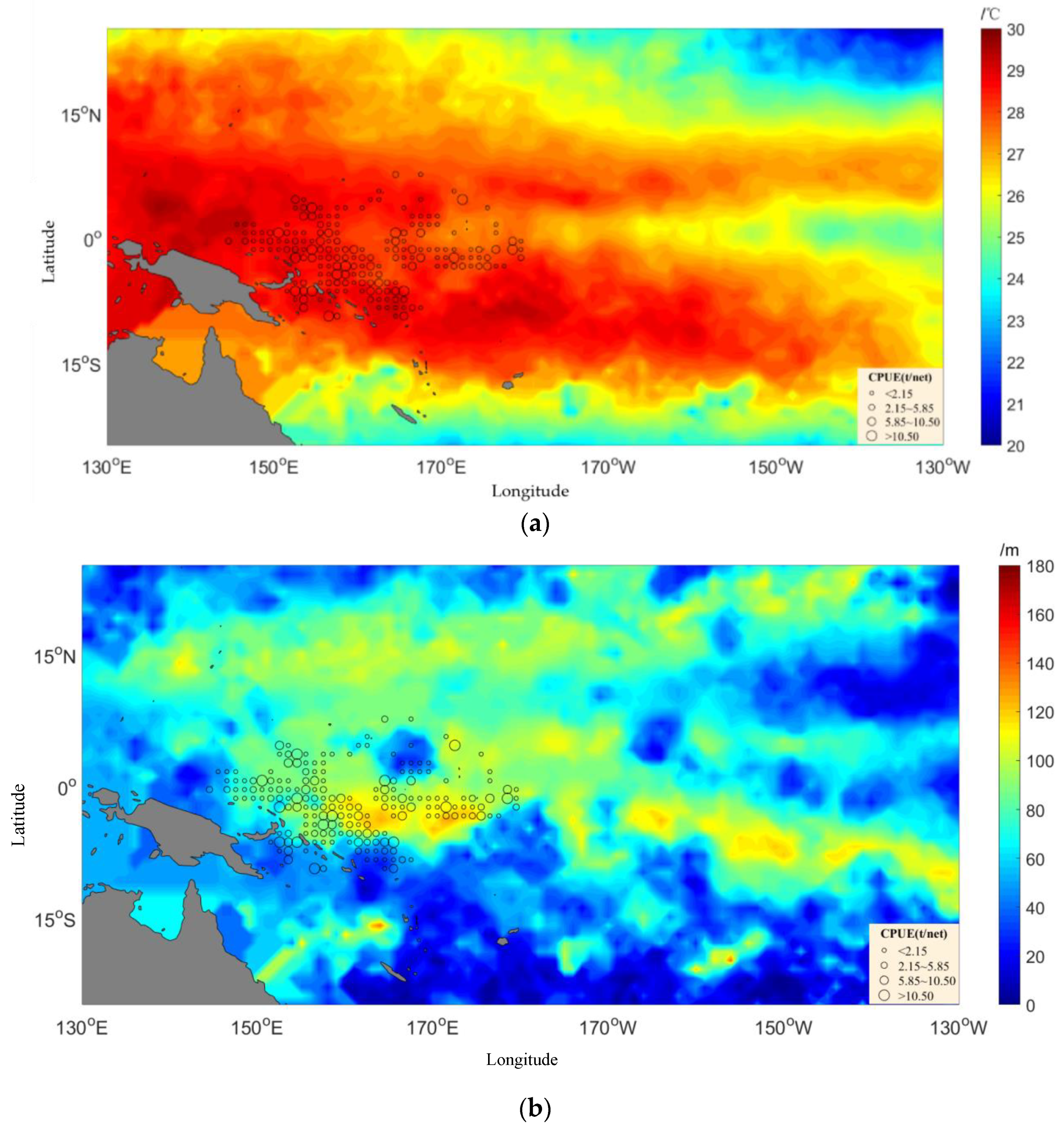
3.1. Temporal and Spatial Variation of Upper Boundary Temperature and Depth of the Thermocline with Catch

The ENSO had a significant impact on the spatial distribution of the yellowfin tuna purse-seine fishing grounds in the WCPO. The superposition of thermocline parameters in a typical La Niña year (2010), normal year (2013), and El Niño year (2015) and the CPUE of yellowfin tuna were analyzed. The results (Figure 1) show that in the La Niña year, the high-value zone of 28–29 °C of the upper boundary temperature of the thermocline moved westward. The CPUE moved westward to the west of 170° E as the high-value zone of the upper boundary temperature contracted westward to 145° E. In the El Niño year, the high-value zone of 28–29 °C of the upper boundary temperature of the thermocline expanded eastward. The CPUE moved eastward to the east of 165° E with the eastward expansion of the high-value zone of the upper boundary temperature to 173° W. Yellowfin tuna is a warm-water fish species whose habitat and spawning area need to be above a certain water temperature. Therefore, the upper boundary temperature of the thermocline will affect the spatial distribution of yellowfin tuna [25].

In the normal year (2013), the upper boundary depth of the thermocline in the equatorial Pacific was deeper in the west and shallower in the east. In the typical La Niña year (2010) compared with the normal year (2013), the upper boundary depth difference of the thermocline on the east and west sides of the equatorial WCPO was larger. The upper boundary depth of 80–130 m was shifted westward, which may have been due to the enhancement of Walker circulation and southeast trade winds in the La Niña year. In the El Niño year (2015) compared with the normal year, the difference of the upper boundary depth of the thermocline on the east and west sides of the equatorial WCPO in the El Niño year was smaller. The upper boundary depth of 80–130 m moved eastward.

3.2. Temporal and Spatial Variation of Thermocline Strength and Thickness with Catch

As shown in Figure 2, the thermocline strength was weaker in the west and stronger in the east. The thermocline strength in the La Niña year was greater than that in the El Niño year in the area of 180° W of the equatorial WCPO. Conversely, the thermocline strength in the La Niña year was less than that in the El Niño year in the area of the 180° E region. On the whole, the thermocline thickness was greater in the west and lesser in the east. There was a thick band-like structure on each side, with an axis of 15° N and 15° S. The CPUE was mainly distributed in the thickness of 120–200 m. Figure 3 illustrates how the maximum CPUE value of yellowfin tuna was shifted westward in longitude and southward in latitude in the La Niña year, and shifted eastward in longitude and northward in latitude in the El Niño year.

The annual output was high in La Niña years such as 2008, 2010, 2011, and 2016 (Figure 4). The main operation area was located in the center of the WCPO warm pool in La Niña years. The SST was very suitable for the growth of yellowfin tuna. Therefore, both the catch and resource abundance were high in La Niña years. The annual production was low in El Niño years such as 2009 and 2015. In El Niño years, the western Pacific thermocline became shallower, whereas the eastern and central Pacific thermocline became deeper. In La Niña years, however, the western Pacific thermocline became deeper, whereas the eastern and central Pacific thermocline became shallower. Hence, the thermocline variation would have caused changes in the yellowfin tuna central fishing grounds. The variation patterns between annual catch and CPUE were consistent.

3.3. Analysis Results of the GAM

The GAM was used to analyze the impact of environmental variables on the temporal and spatial variation of yellowfin tuna catch. The results show that the AIC value of the model decreased with the number of factors. The final model retained all the input variables. Meanwhile, the AIC value of the model was the lowest, with a CPUE total variance interpretation of 21.1%, as illustrated in

Table 3. Statistical characteristics of GAM models.

Formulae	AIC	Deviance/%	R2adj
Log(CPUE + 1) = s(y)	11,712.65	13.7	0.135
Log(CPUE + 1) = s(y) + s(m)	11,637.99	15.4	0.151
Log(CPUE + 1) = s(y) + s(m) + s(lat)	11,570.29	16.8	0.164
Log(CPUE + 1) = s(y) + s(m) + s(lat) + s(lon)	11,521.25	17.9	0.174
Log(CPUE + 1) = s(y) + s(m) + s(lat) + s(lon) + s(upt)	11,485.4	18.6	0.181
Log(CPUE + 1) = s(y) + s(m) + s(lat) + s(lon) + s(upt) + s(dh)	11,472.67	18.9	0.184
Log(CPUE + 1) = s(y) + s(m) + s(lat) + s(lon) + s(upt) + s(dh) + s(uph)	11,468.99	19.1	0.186
Log(CPUE + 1) = s(y) + s(m) + s(lat) + s(lon) + s(upt) + s(dh) + s(uph) + s(intensity)	11,458.37	19.2	0.187
Log(CPUE + 1) = s(y) + s(m) + s(lat) + s(lon) + s(upt) + s(dh) + s(uph) + s(intensity) + s(ONI)	11,361.8	21.1	0.205

Note: y—year; m—month; lat—latitude; lon—longitude; upt—upper temperature of the thermocline; uph—upper depth of the thermocline; dh—thickness of the thermocline; intensity—strength of the thermocline; ONI—Oceanic Niño Index; GAM—generalized additive models.

. In the model, the contribution of variables explaining the change in CPUE indicated the degree of impact on CPUE. The contribution of the time factor was 15.4%, that of the spatial factor was 2.5%, and that of the environmental factors was 3.2% (

Table 4. Test values of generalized additive models (GAM).

Variable	edf	Ref. df	F	P	Contribution Rate (%)
Year	8.046	8.757	75.019	<0.001	13.7
Month	6.394	7.550	6.030	2.72 × 10−7	1.7
Latitude	4.757	5.809	12.212	5.51 × 10−13	1.4
Longitude	5.768	6.783	10.550	3.27 × 10−12	1.1
Upper temperature	1.000	1.000	9.311	0.002 29	0.7
Thickness of thermocline	1.000	1.000	1.052	0.305 02	0.3
Upper depth of thermocline	1.000	1.000	0.287	0.592 13	0.2
Intensity	1.000	1.001	9.390	0.002 19	0.1
ONI	8.109	8.750	14.491	<0.001	1.9

). The year was the most important factor, followed by the ONI, month, latitude, longitude, and upper boundary temperature and depth of thermocline, whereas thermocline strength and thickness had little impact on the GAM.

The effects of spatial and temporal variables on the CPUE were nonlinear, whereas the effects of the upper boundary temperature and depth of the thermocline and thermocline thickness and strength on the CPUE among environmental variables were linear (Figure 5). As shown in Figure 5, (1) the purse-seine CPUE of yellowfin tuna decreased from 2008 to 2009, barely fluctuated from 2009 to 2010, decreased from 2011 to 2012, and then increased by 2016. Hence, the impact of the year on the CPUE fluctuated. The confidence intervals were narrow in 2008, 2011, and 2013, indicating that those La Niña years had a strong impact on the CPUE. (2) The CPUE of yellowfin tuna changed little in different months. It remained unchanged from January to April, increased slightly by June, and then began to fluctuate. (3) The impact curve of latitude on the CPUE presented a dome shape. The CPUE value was the largest in the 0° equatorial region. The 95% confidence interval was narrow, and the confidence level was high. The CPUE increased with latitude from 10° S–0° and decreased with latitude from 0–5° N, showing that the CPUE increased gradually as the latitude approached the equator. (4) The CPUE increased with the increase in longitude from 140–150° E. However, the confidence interval was large, and the confidence level was low. The CPUE fluctuated and the confidence interval was narrow at 150–175° E, indicating that the meridional space close to the CPUE was 150–175° E. Moreover, the confidence level dropped with the increase in longitude and the expansion of the confidence interval in the east of 175° E.

Among the environmental variables, the relationship between the upper boundary temperature of the thermocline and the CPUE showed that the upper boundary temperature of the thermocline in the yellowfin tuna fishing grounds was between 27 and 30 °C, with an optimal upper boundary temperature range of 27.5–29.5 °C. The upper boundary depth of the thermocline was between 50 and 150 m. The optimal upper boundary depth range was 80–120 m. The thermocline thickness of the fishing grounds was between 100 and 200 m. The CPUE increased with the thickness of the thermocline. However, the confidence interval increased, and the confidence level decreased. The thermocline strength of fishing grounds was between 0.08 and 0.13 °C·m⁻¹ and was positively correlated with the CPUE. The CPUE increased with the increase in ONI, and 0.3 was the maximum value. ONI in the range of −1–0.6 was closely related to CPUE.

4. Discussion

Temperature is a key environmental factor affecting fish activities [28]. It can directly and indirectly affect fish life activities, such as spawning [29], embryonic development [30,31], survival rate [32], feeding metabolism [33], migration [34], and habitat distribution [35]. Yellowfin tuna is a warm-water fish species that needs a certain water temperature to inhabit and spawn. The temporal and spatial variation of thermocline characteristic parameters of yellowfin tuna fishing grounds in the WCPO in El Niño and La Niña years shows that the CPUE in a La Niña year moved westward to 170° E as the high-value zone of the upper boundary temperature contracted westward to 145° E. In an El Niño year, the CPUE moved eastward with the eastward expansion of the high-value zone of the upper boundary temperature, which generally moved eastward to the east of 165° E. The reason may be that the upper boundary temperature of the thermocline affects the tuna spatial distribution. The high-value zone of 27–29.5 °C of the upper boundary temperature in El Niño years expanded eastward, whereas that in La Niña years moved westward. Furthermore, changes in the vertical structure of the water temperature profile also affect the horizontal spatial distribution and fishing mode for tuna [36]. To summarize, the CPUE distribution of fishing grounds in El Niño and La Niña years change with the eastward expansion or westward shift, respectively, of the upper boundary temperature of the thermocline, which makes new areas suitable for fishing grounds. Thermocline changes in the tropical Pacific are caused by SSTAs, which consist of enhanced deep atmospheric convection and westerly wind anomalies in the central Pacific. During all El Niño events, weaker equatorial trade winds produce an eastward shift of the western Pacific warm pool, and a deeper thermocline response to this wind anomaly in turn reinforces the initial warming. Sea-level anomalies in this area exhibit a zonal seesaw indicative of a deeper (shallower) thermocline in the eastern (western) equatorial Pacific [37,38]. The strong temperature gradient of the thermocline is a physical barrier for skipjack and juvenile yellowfin and bigeye tuna, whereas adult yellowfin and bigeye tuna can dive below the thermocline to chase mesopelagic prey. Therefore, changes in the vertical thermal structure of the ocean associated with ENSO can potentially impact the catchability of tuna species by different fishing gears. Purse seiners targeting surface tuna use the top of the thermocline as a lower barrier to trap tuna schools [39].

In order to accurately analyze the relationship between the abnormal climate phenomena and the abundance and spatial-temporal distribution of yellowfin tuna resources in the WCPO, this study explored the impacts of environmental variables on the temporal and spatial variation in yellowfin tuna catch by using a generalized additive model (GAM) and analyzing the optimal environmental parameters of the thermocline where the fishing grounds were located. The results showed that the contribution of the time factor was 15.4%, that of the spatial factor was 2.5%, and that of the environmental factors was 3.2%. The upper boundary temperature of the thermocline in yellowfin tuna fishing grounds was mostly between 27 and 30 °C. The optimal upper boundary temperature range was 27.5–29.5 °C. The upper boundary temperature of the thermocline had the greatest impact among the subsurface environmental factors.

According to the analysis results of spatial superposition and the GAM, the thermocline strength in the WCPO was weaker in the west and stronger in the east. The 180° W region of the equatorial WCPO was the main fishing area in which the thermocline strength in La Niña years was greater than that in El Niño years. Conversely, the thermocline strength in La Niña years was less than that in El Niño years in the 180° E region. Moreover, the CPUE was closely related to the thermocline in the strength range of 0.08–0.13 °C·m⁻¹.

Regarding the upper boundary depth of the thermocline, the thermocline was thicker in the west and thinner in the east. There was a thick band-like structure on each side with an axis spanning 15° N and 15° S. The CPUE was distributed in the range of 120–200 m. The width of the thermocline in the WCPO in La Niña years was lesser than in El Niño years. GAM analysis showed that the upper boundary depth of the thermocline where the fishing grounds were located was between 50 and 150 m. In addition, the optimal upper boundary depth of the thermocline where the fishing grounds were located ranged from 80 to 120 m, which was consistent with the 70–109 m suitable upper boundary depth of the thermocline for yellowfin tuna in the WCPO [40]. Compared with the normal years, the upper boundary depth difference of the thermocline on the east and west sides of the equatorial WCPO was larger in La Niña years, and the upper boundary depth value of 80–130 m was shifted westward. Compared with normal years, the upper boundary depth difference of the thermocline on the east and west sides of the equatorial WCPO decreased in El Niño years. The upper boundary depth value of 80–130 m moved eastward.

Studies [41,42] have suggested that the center of gravity of the catch in the WCPO moves eastward and southward in El Niño years, and moves slightly westward and northward in La Niña years. This is consistent with the conclusion of this study for longitude. The slight difference in latitude may be the result of different research objects. The research object of this paper was yellowfin tuna, whereas other studies in the literature [28] considered skipjack tuna. Moreover, the time series of the research data were inconsistent. The data used in this article are relatively updated data, which may also have led to differences. According to the statistical results of the catch in this paper, the yield in La Niña years was higher than that in El Niño years. Chen et al. [43] found that the yield was higher in La Niña years and lower in El Niño years when studying the effects of El Niño and La Niña on skipjack abundance in the WCPO. Deary et al. [44] also found that the production of yellowfin tuna in the central Pacific increased significantly in La Niña years. This may be because the upper boundary depth of the thermocline in the WCPO in La Niña years is deeper than in El Niño years, and the thermocline strength is higher than in El Niño years. In La Niña years, the suitable vertical habitat space of yellowfin tuna in this area is compressed, which is conducive to surface fishing and high catch. In contrast, the catch is lower during El Niño years [45,46]. In addition, the vertical structure of the thermocline has little impact on the fishing ground due to purse-seine operation. However, the thermocline changes caused by abnormal climate events have significant impacts on the CPUE. This study provides a reference for purse-seine tuna production in the tropical WCPO in abnormal climate years and for the study of the relationship between the temporal and spatial distribution of tuna and the thermocline.

References

1. FAO. The State of Food and Agriculture 2020. Overcoming Water Challenges in Agriculture; FAO: Rome, Italy, 2020. [Google Scholar]
2. McKinney, R.; Gibbon, J.; Wozniak, E.; Galland, G. Netting Billions 2020: A Global Tuna Valuation; The Pew Charitable Trusts: Philadelphia, PA, USA, 2020. [Google Scholar]
3. McCluney, J.K.; Anderson, C.M.; Anderson, J.L. The fishery performance indicators for global tuna fisheries. Nat. Commun. 2019, 10, 1641. [Google Scholar] [CrossRef] [PubMed] [Green Version]
4. FFA Tuna Development Indicators 2016. Available online: https://www.ffa.int/system/files/FFATunaDevelopmentIndicatorsBrochure.pdf (accessed on 11 January 2022).
5. Lehodey, P.; Senina, I.; Calmettes, B.; Hampton, J.; Nicol, S. Modelling the impact of climate change on Pacific skipjack tuna population and fisheries. Clim. Chang. 2013, 119, 95–109. [Google Scholar] [CrossRef]
6. Clark, S.; Bell, J.; Adams, T.; Allain, V.; Aqorau, T.; Hanich, Q.; Jaiteh, V.; Lehodey, P.; Pilling, G.; Senina, I.; et al. The Parties to the Nauru Agreement (PNA) ‘Vessel Day Scheme’: A cooperative fishery management mechanism assisting member countries to adapt to climate variability and change. In Fisheries and Aquaculture Technical Paper 667. Adaptive Management of Fisheries in Response to Climate Change; FAO: Rome, Italy, 2021; pp. 209–224. [Google Scholar]
7. Asch, R.G.; Cheung, W.W.L.; Reygondeau, G. Future marine ecosystem drivers, biodiversity, and fisheries maximum catch potential in Pacific Island countries and territories under climate change. Mar. Policy 2018, 88, 285–294. [Google Scholar] [CrossRef]
8. Lam, V.W.Y.; Allison, E.H.; Bell, J.D.; Blythe, J.; Cheung, W.W.L.; Frölicher, T.L.; Gasalla, M.A.; Sumaila, U.R. Climate change, tropical fisheries and prospects for sustainable development. Nat. Rev. Earth Environ. 2020, 1, 440–454. [Google Scholar] [CrossRef]
9. Cai, W.J.; Borlace, S.; Lengaigne, M.; Rensch, P.V.; Collins, M.; Vecchi, G.; Timmermann, A.; Santoso, A.; McPhaden, M.J.; Wu, L.X.; et al. Increasing frequency of extreme El Niño events due to greenhouse warming. Nat. Clim. Chang. 2014, 4, 111–116. [Google Scholar] [CrossRef] [Green Version]
10. Lehodey, P.; Bertignac, M.; Hampton, J.; Lewis, A.; Picaut, J. El Niño Southern Oscillation and tuna in the western Pacific. Nature 1997, 389, 715–718. [Google Scholar] [CrossRef]
11. Hampton, J.; Lewis, A.; Williams, P. The Western and Central Pacific Tuna Fishery: Overview and Status of Stocks; Oceanic Fisheries Programme; Secretariat of the Pacific Community: Nouméa, New Caledonia, 1999; Volume 39. [Google Scholar]
12. Hampton, J. Estimates of tag-reporting and tag-shedding rates in a large-scale tuna tagging experiment in the western tropical Pacific Ocean. Oceanogr. Lit. Rev. 1997, 11, 1346. [Google Scholar]
13. Climate Variability. Oceanic Niño Index. Available online: https://www.climate.gov/news-features/understanding-climate/climate-variability-oceanic-ni%C3%B1o-index (accessed on 11 January 2022).
14. Watters, G.M.; Hinke, J.T.; Reiss, C.S. Long-term observations from Antarctica demonstrate that mismatched scales of fisheries management and predator-prey interaction lead to erroneous conclusions about precaution. Sci. Rep. 2020, 10, 2314. [Google Scholar] [CrossRef] [Green Version]
15. Lan, K.W.; Lee, M.A.; Zhang, C.I.; Wang, P.Y.; Wu, L.J.; Lee, K.T. Effects of climate variability and climate change on the fishing conditions for grey mullet (Mugil cephalus L.) in the Taiwan Strait. Clim. Chang. 2014, 126, 189–202. [Google Scholar] [CrossRef] [Green Version]
16. Li, H.; Xu, F.; Zhou, W.; Wang, D.; Wright, J.S.; Liu, Z.; Lin, Y. Development of a global gridded Argo data set with B arnes successive corrections. Geophys. Res. Ocean. 2017, 122, 866–889. [Google Scholar] [CrossRef]
17. Liu, S.L.; Liu, Z.D.; Li, H.; Li, Z.Q.; Wu, X.F.; Sun, C.H.; Xu, J.P. Manual of Global Ocean Argo gridded data set. Geophys. Res. Ocean. 2020, 122, 14. [Google Scholar]
18. Akima, H.A. New Method of Interpolation and Smooth Curve Fitting Based on Local Procedures. J. ACM (JACM) 1970, 17, 589–602. [Google Scholar] [CrossRef]
19. Zhou, Y.X.; Li, B.L.; Zhang, Y.J.; Ba, N.C. World oceanic thermocline characteristics in winter and summer. Mar. Sci. Bull. 2002, 21, 16–22. [Google Scholar]
20. Guisan, A.; Edwards, J.T.C.; Hastie, T. Generalized linear and generalized additive models in studies of species distributions: Setting the scene. Ecol. Model. 2002, 157, 89–100. [Google Scholar] [CrossRef] [Green Version]
21. Mainuddin, M.; Ssiton, K.; Saiton, S.I. Albacore fishing ground in relation to oceanographic conditions in the western North Pacific Ocean using remotely sensed satellite data. Fish Oceanogr. 2008, 17, 61–73. [Google Scholar] [CrossRef] [Green Version]
22. Briand, K.; Molony, B.; Lehodey, P. A study on the variability of albacore (Thunnus alalunga) longline catch rates in the southwest Pacific Ocean. Fish Oceanogr. 2011, 20, 517–529. [Google Scholar] [CrossRef]
23. Wu, S.N.; Chen, X.J.; Liu, Z.N. Establishment of forecasting model of the abundance index for chub mackerel (Scomber japonicus) in the northwest Pacific Ocean based on GAM. Acta Oceanol. Sin. 2019, 41, 36–42. [Google Scholar]
24. Yu, J.; Hu, Q.; Tang, D.; Pimao, C. Environmental effects on the spatiotemporal variability of purpleback flying squid in Xisha-Zhongsha waters, South China Sea. Mar. Ecol. Prog. Ser. 2019, 623, 25–37. [Google Scholar] [CrossRef]
25. Yang, S.L.; Zhang, B.B.; Tang, B.J.; Hua, C.J.; Zhang, S.M.; Fang, X.M.; Dai, Y.; Feng, C.L. Influence of vertical structure of the water temperature on bigeye tuna longline catch rates in the tropical Atlantic Ocean. Fish Sci. China 2017, 4, 875–883. [Google Scholar]
26. Wood, S.N. Generalized Additive Models: An Introduction with R, 2nd ed.; Chapman & Hall/CRC: Boca Raton, FL, USA, 2017; p. 476. [Google Scholar]
27. Historical El Niño/La Niña Episodes (1950-Present). Available online: https://origin.cpc.ncep.noaa.gov/products/precip/CWlink/MJO/enso.shtml (accessed on 11 January 2022).
28. Dai, D.N.; Liu, H.S.; Dai, X.J.; Tian, S.Q. The relationship between ENSO and spatio-temporal distribution of CPUE of yellowfin tuna (Thunnus albacares) by purse seine in the Eastern Pacific Ocean. Shanghai Ocean Univ. 2011, 20, 571–578. [Google Scholar]
29. Kurita, Y.; Fujinami, Y.; Amano, M. The effect of temperature on the duration of spawning markers—Migratory-nucleus and hydrated oocytes and postovulatory follicles—In the multiple-batch spawner Japanese flounder (Paralichthys olivaceus). Fish. Bull. 2011, 109, 79–89. [Google Scholar]
30. Arenzon, A.; Lemos, C.A.; Bohrer, M. The influence of temperature on the embryonic development of the annual fish cynopoecilus melanotaenia (cyprinodontiformes, rivulidae). Braz. J. Biol. 2002, 62, 743. [Google Scholar] [CrossRef] [Green Version]
31. Schirone, R.C.; Gross, L. Effect of temperature on early embryological development of the zebra fish, Brachydanio rerio. J. Exp. Zool. Part A Ecol. Integr. Physiol. 1968, 169, 43–52. [Google Scholar] [CrossRef]
32. Emilie, R.D.; Alain, P.; Daniel, D.C.; Pascal, F.; Fabrice, T.; Rummer, J.L. Strong effects of temperature on the early life stages of a cold stenothermal fish species, brown trout (Salmo trutta L.). PLoS ONE 2016, 11, e0155487. [Google Scholar]
33. Jobling, M. The influences of feeding on the metabolic rate of fishes: A short review. J. Fish Biol. 1981, 18, 385–400. [Google Scholar] [CrossRef]
34. Jansen, T.; Gislason, H. Temperature affects the timing of spawning and migration of north sea mackerel. Cont. Shelf Res. 2011, 31, 64–72. [Google Scholar] [CrossRef]
35. Freitas, C.; David, V.R.; Moland, E.; Olsen, E.M. Sea temperature effects on depth use and habitat selection in a marine fish community. J. Anim. Ecol. 2021, 90, 1787–1800. [Google Scholar] [CrossRef]
36. Yang, S.L.; Zhang, B.B.; Zhang, H.; Zhang, S.M.; Wu, Y.M.; Zhou, W.F.; Feng, C.L. A Review: Vertical Swimming and Distribution of Yellowfin Tuna Thunnus alalunga. Fish. Sci. 2019, 38, 119–126. [Google Scholar]
37. Barnston, A.G.; Tippett, M.K.; L’Heureux, M.L.; Li, S.; DeWitt, D.G. Skill of real-time seasonal ENSO model predictions during 2002–11: Is our capability increasing? Bull. Am. Meteorol. Soc. 2012, 93, 631–651. [Google Scholar] [CrossRef]
38. Kirtman, B.P.; Min, D.; Infanti, J.M.; Kinter, J.L., III; Paolino, D.A.; Zhang, Q.; van den Dool, H.; Saha, S.; Mendez, M.P.; Becker, E.; et al. The North American Multimodel Ensemble: Phase-1 Seasonal-to-Interannual Prediction; Phase-2 toward Developing Intraseasonal Prediction. Bull. Am. Meteorol. Soc. 2014, 95, 585–601. [Google Scholar] [CrossRef]
39. Lehodey, P.; Bertrand, A.; Hobday, A.J.; Kiyofuji, H.; McClatchie, S.; Menkès, C.E.; Pilling, G.; Polovina, J.; Tommasi, D. ENSO Impact on Marine Fisheries and Ecosystems. In El Niño Southern Oscillation in a Changing Climate; McPhaden, M.J., Santoso, A., Cai, W., Eds.; AGU and John Wiley & Sons: Washington, DC, USA; New York, NY, USA, 2020; pp. 429–451. [Google Scholar]
40. Yang, S.L.; Zhang, B.B.; Jin, S.F.; Fan, W. Relationship between the temporal-spatial distribution of longline fishing grounds of yellowfin tuna (Thunnus albacares) and the thermocline characteristics in the Western and Central Pacific Ocean. Acta Oceanol. Sin. 2015, 37, 78–87. [Google Scholar]
41. Shen, J.H.; Chen, X.D.; Cui, X.S. Analysis on spatial-temporal distribution of skipjack tuna catches by purse seine in the Western and Central Pacific Ocean. Mar. Fish. 2006, 1, 13–19. [Google Scholar]
42. Guo, A.; Chen, X.J. The relationship between ENSO and tuna purse-seine resource abundance and fishing grounds distribution in the Western and Centra1 Pacific Ocean. Mar. Fish. 2005, 27, 338–342. [Google Scholar]
43. Chen, Y.Y.; Chen, X.J. Influence of El Nino/La Nina on the abundance index of skipjack in the Western and Central Pacific Ocean. Shanghai Ocean Univ. 2017, 26, 113–120. [Google Scholar] [CrossRef]
44. Deary, A.L.; Moret, F.S.; Engels, M.; Zettler, E.; Jaroslow, G.; Sancho, Y.G. Influence of Central Pacific Oceanographic Conditions on the Potential Vertical Habitat of Four Tropical Tuna Species1. Pac. Sci. 2015, 69, 461–476. [Google Scholar] [CrossRef] [Green Version]
45. Prince, E.D.; Goodyear, C.P. Hypoxia-based habitat compression of tropical pelagic fishes. Fish Oceanogr. 2006, 15, 451–464. [Google Scholar] [CrossRef]
46. Prince, E.D.; Luo, J.; Phillip, G.C.; Hoolihan, J.P.; Snodgrass, D.; Orbesen, E.S.; Serafy, J.E.; Ortiz, M.; Schirripa, M.J. Ocean scale hypoxia-based habitat compression of Atlantic istiophorid billfishes. Fish Oceanogr. 2010, 19, 448–462. [Google Scholar] [CrossRef]
Figure 1. Overlay distribution of the upper temperature of the thermocline, the upper depth of the thermocline, and the catch per unit effort (CPUE) of yellowfin tuna. (a) The upper temperature of the thermocline in a La Niña year (2010); (b) the upper depth of the thermocline in a La Niña year (2010); (c) the upper temperature of the thermocline in a normal year (2013); (d) the upper depth of the thermocline in a normal year (2013); (e) the upper temperature of the thermocline in an El Niño year (2015); (f) the upper depth of the thermocline in an El Niño year (2015).
Sustainability 14 01217 g001aSustainability 14 01217 g001bSustainability 14 01217 g001c
Figure 2. Overlay distribution of the strength and thickness of the thermocline and the catch per unit effort (CPUE) of yellowfin tuna. (a) The strength of the thermocline in a La Niña year (2010); (b) the thickness of the thermocline in a La Niña year (2010); (c) the strength of the thermocline in a normal year (2013); (d) the thickness of the thermocline in a normal year (2013); (e) the strength of the thermocline in an El Niño year (2015); (f) the thickness of the thermocline in an El Niño year (2015).
Sustainability 14 01217 g002aSustainability 14 01217 g002b
Figure 3. Distribution of catch per unit effort (CPUE) with longitude (a) and latitude (b) for yellowfin tuna in the central and western Pacific.
Sustainability 14 01217 g003
Figure 4. Annual catch and catch per unit effort (CPUE) statistics of yellowfin tuna in the central and western Pacific.
Sustainability 14 01217 g004
Figure 5. Effects of predictor variables: (a) year, (b) month, (c) Latitude, (d) Longitude, (e) thermocline upper temperature, (f) thermocline upper depth, (g) Thermocline thickness, (h) thermocline strength, and (i) the Oceanic Niño Index, derived from the generalized additive model (GAM) on catch per unit effort (CPUE).
Sustainability 14 01217 g005