Ecosystems Services and Green Infrastructure for Respiratory Health Protection: A Data Science Approach for Paraná, Brazil

Abstract

Urban ecosystem services have become a main issue in contemporary urban sustainable development, whose efforts are challenged by the phenomena of world urbanization and climate change. This article presents a study about the ecosystem services of green infrastructure towards better respiratory health in a socioeconomic scenario typical of the Global South countries. The study involved a data science approach comprising basic and multivariate statistical analysis, as well as data mining, for the municipalities of the state of Paraná, in Brazil’s South region. It is a cross-sectional study in which multiple data sets are combined and analyzed to uncover relationships or patterns. Data were extracted from national public domain databases. We found that, on average, the municipalities with more area of biodiversity per inhabitant have lower rates of hospitalizations resulting from respiratory diseases (CID-10 X). The biodiversity index correlates inversely with the rates of hospitalizations. The data analysis also demonstrated the importance of socioeconomic issues in the environmental-respiratory health phenomena. The data mining analysis revealed interesting associative rules consistent with the learning from the basic statistics and multivariate analysis. Our findings suggest that green infrastructure provides ecosystem services towards better respiratory health, but these are entwined with socioeconomics issues. These results can support public policies towards environmental and health sustainable management.

1. Introduction

The sustainability concept is multidimensional and encompasses social, ecological and economic theories, policies and practices. The phenomena of world urbanization and climate change challenge sustainable development efforts. In that matter, the thematic of ecosystems services provided by urban green infrastructure (UGI), as in nature-based solutions, have been argued to act transversally and with positive impacts in all dimensions of sustainability. This is in the center of the debate of the contemporary city development agenda towards sustainability [1,2,3,4].

Ecosystem services (ES) include all the interlinked aspects of ecological structures with functions that are advantageous and bring benefits to human wellbeing [5]. ES also encompass social capital [6,7]. These ecological structures aim to reduce urban risks and are formed by interconnected green spaces that have been referred to more recently as UGI.

Squares, parks, planned gardens, forest reserves, fragments of original or secondary forest, urban woods, afforested streets, among others, compose UGI [8]. Also, innovative methods of planning and placing these green spaces in the urban environment have been developed, especially with the interests of adding to rainwater drainage and water quality management [9]. Some examples are green walls and roofs, wells and ditches for infiltration and bio-retention, and sidewalks and pavements that allow infiltration.

UGI contribute to the actions to mitigate and adapt to climate change [10]. They reduce the risks of natural disasters and contribute to the improvement of urban planning [11]. And acts on environmental urban stressors related in many ways to human health, such as noise and air pollution, as well as heat islands and waves [12,13,14], and to reduce air pollution that increase the risks and is many times associated with the occurrence of respiratory diseases [15].

Air pollution is a significant global problem and has become a threat to human health and the climate. Worldwide, more than 200 million people suffer from chronic obstructive pulmonary disease (COPD) [16], and the World Health Organization (WHO) highlighted that pollution is estimated to be responsible for 4.2 million deaths per year, with (COPD) accounting for 43% of the total. Asthma in children is related and may be aggravated under air pollution exposure. It also increases the chances of developing COPD late in adult life [17]. Both short- and long-term exposure to air pollution may reduce pulmonary function and cause infections [18]

There is a vast body of literature that discusses the impact of vegetation on the reduction of air pollution (e.g., [15]). Other authors, however, such as [19,20], argue that there are conflicting factors involved in the direct association between urban vegetation and the risks of respiratory diseases. Plants and trees affect the air quality through pollen emissions, which can cause allergies. In addition, some species of trees are responsible for high emissions of biogenic volatile organic compounds (B-VOCs) that can result in ozone formation and can also combine with the VOCs of anthropogenic sources, which along with the dispersed pollen, may aggravate or cause respiratory diseases [21,22].

More recently, there has been increasing research focused in the direct effects of vegetation on respiratory health, mainly associated with urbanization, climate change and the increase of air pollution [23,24,25,26,27,28]. In addition, as the urban environment is man-made, the species of vegetation, the dynamics that take place in their biochemistry cycles and soil-plant-atmosphere interactions, the way they are dispersed, as well as the pollution sources (typology and location), dynamics of city life, weather conditions, season, and climate can all influence the atmospheric circulation and air flow. This may limit the dispersal of the pollutants and allergenic particles, contributing to the onset or aggravation of respiratory conditions [23,29,30]. Therefore, it remains controversial whether or not vegetation can be beneficial to respiratory health [31].

In addition, socioeconomic factors are also known to be powerful determinants of health [32,33]. Public health issues result in high costs for society, limiting urban sustainable development. These issues restrict childhood development with the loss of school days and lower working productivity due to absenteeism, especially that caused by hospitalizations.

The hypothesis underlying this research is that UGI acts as a protection from respiratory health. The main goal is to study the direct benefits of UGI in diminishing hospitalizations because of respiratory diseases, considering also the socioeconomic scenario of the Global South countries. The approach involves data science, and the application of a data-mining algorithm, seeking relationships or patterns in a multiple data set, which includes mainly demography, socioeconomic and UGI indicators. It also addresses the need for a more comprehensive environmental perspective associated with urban management and health.

2. Materials and Methods

2.1. Study Area

Paraná is a state located in the southern region of Brazil (Figure 1) that is composed of 399 municipalities. The state of Paraná shares borders with Argentina and Paraguay in South America. In area, Paraná (199,315 km²) is smaller than the state of São Paulo (approximately 248,000 km²) in Brazil and the territory of New Zealand (268,021 km²) in Oceania, yet is approximately the same size as Senegal in West Africa (196,712 km²).

According to the last census in 2010, the total population of the state was 10,444,526 inhabitants [34], the sixth largest in Brazil, which corresponds to approximately 5% of the total population. This is approximately 25% of the population of the state of São Paulo (41,262,199 inhabitants in 2010) and more than double that of New Zealand. The main city is Curitiba (25°25′40″ S, 49°16′23″ W), which is one of the 10 cities that comprise 40% of the state’s total population.

The northwestern part of the central and southeastern regions, as well as nearly all of the southwestern region of the State of Paraná are in a subtropical climate (Cfa) according to the Köppen classification, with average temperatures of under 18 °C in the coldest month, and above 22 °C in the warmest, with hot summers. Meanwhile, approximately half of the central, southeastern, and southern regions of the state have a temperate climate (Cfb), with average temperatures of under 18 °C in the coldest month, and fresh summers, with average temperatures of under 22 °C and without a defined dry season [35].

The State of Paraná has the fifth largest economy in the country. The pressure on land use change comes from the natural potential for hydropower generation and for agriculture. It is home to the Itaipu dam, the second largest in the world, which generates energy for both Brazil and Paraguay. Agribusiness is very relevant in Paraná, and dairy and meat production add important industrial value to its economy. Paraná ranks among the top ten Brazilian exporting states; its municipal average Gross Domestic Product was 26,058 BRL in 2015 (equivalent to approximately 6950 USD on 15 November 2018), which comes mostly from soybean exports (Brazil presented the world largest soybean production in 2020/2021). The Human Development Index (HDI) was 0.749 in 2010, which is above the country’s average of 0.699 [34,36].

With regards to respiratory diseases (CID-10 X), the southern region of Brazil has the highest hospitalization rates, and Paraná, one of the three states in this region, generally presents the highest rates. In 2016, respiratory diseases were the third highest cause of morbidity in the state [37]. It was noticeable that circulatory diseases, which are the main cause of death globally, were correlated with respiratory diseases in Paraná (e.g., [27]). In 2016, circulatory diseases (CID-10 IX) were the second highest cause of hospitalizations in Paraná, supplanted only by pregnancy, childbirth, and puerperium (CID-10 XV).

2.2. Research Methods

The method involved the application of data mining techniques, which is usually divided into three main steps: data acquisition, preparation, and analysis. The analysis, in this case, involved the classification and extraction of association rules in order to acquire knowledge about the ecosystem services that UGI can provide to protect respiratory health. This was preceded by basic and multivariate statistical analysis. Initially, the data to be considered for mining were not fully known. Therefore, the whole process was preceded by a survey of possible data and their availability to be used in the study. As health issues are known to be entwined with poverty and with environmental issues [38], the public domain National Health database and the Census database were the first choice for data acquisition. The Brazilian Census of 2010 incorporated an index associated with street trees that was included as an indicator of urban green infrastructure. Apart from that, for the same year, there were data about the biodiverse areas in municipalities, considered as a second indicator of urban green infrastructure, as well as data about licensed vehicles, which are known to play an important role in air pollution. The selected variables, their sources and preparation are discussed in Section 2.2.1. This is followed by Section 2.2.2, which describes the analysis of categorical data; the basic and multivariate statistics of numerical data; and the description of the mining algorithm for classification, and the extraction of association rules.

2.2.1. Data Acquisition and Preparation

Table 1. Variables, description and sources.

Variable	Type	Description	Unit	Source
MUN	Categorical	Municipality Name	-	Cidades Platform (IBGE)
SIZE	Categorical	Municipality classification according to the population range	-	IBGE
TYPOLOGY	Categorical	Municipality typology rural-urban	-	IBGE
TOT_POP	Numerical	Number of people living in the municipality	number of persons	Cidades Platform (IBGE)
URBAN_POP	Numerical	Number of people living in areas designated as urban divided by the total population	ratio	SIDRA Platform (IBGE). Estimate from Table 207 of the 2010 Census.
DEMO_DENS	Numerical	TOT_POP divided by the area of the municipality	Number of persons per square kilometer	Cidades Platform (IBGE)
M_HDI	Numerical	Municipal Human Development Index	Ratio (0 to 1)	Cidades Platform (IBGE)
low_INCOME	Numerical	Number of households with a monthly income of up to half the Brazilian Minimum Salary in 2010, divided by the total households in the municipality	ratio	SIDRA Platform (IBGE). Table 3268 of the 2010 Census.
GDP_USDOLARS	Numerical	Gross Domestic Product per capita	USD	Cidades Platform (IBGE)
SAN	Numerical	Number of households with adequate sanitation divided by the total number of households	ratio	Cidades Platform (IBGE)
ST_TREES	Numerical	Number of people living in households located in urban areas with street trees divided by TOT_POP	ratio	SIDRA Platform (IBGE). Estimate from Table 3362 of the 2010 Census.
URB	Numerical	Number of households with adequate urban ordination (sidewalk, curb, paved streets) divided by the total number of households	ratio	Cidades Platform (IBGE)
BIODIVERSITY	Numerical	Hectares of biodiversity conservation unit divided by TOT_POP	ha/inhab	DIBAP/ICMS IAT-PR (http://www.iat.pr.gov.br/Pagina/ICMS-Ecologico-por-Biodiversidade (accessed on 14 October 2021); http://www.iat.pr.gov.br/sites/agua-terra/arquivos_restritos/files/documento/2020-03/repasse_icmse_2017_por_municipio.pdf. (accessed on 14 October 2021))
VHCLS	Numerical	Total number of vehicles divided by TOT_POP	ratio	DENATRAN
RD	Numerical	Number of hospitalizations because of respiratory diseases divided by TOT_POP, times 100	Hospitalizations per 100 inhab	MS/TabNet/DATASUS

presents all the variables studied and their descriptions and sources. The studies included both categorical and numerical variables for each municipality in the state. The categorical variables were the name of the municipality (MUN), designated by an acronym; municipality classification according to its population range (SIZE); and municipality’s rural-urban typology (TYPOLOGY). Meanwhile, the numerical variables involved the rate of people living in areas designated as urban (URBAN_POP), demographic density (DEMO_DENS), gross domestic product (GDP), number of households with a monthly income of up to half the Brazilian Minimum Wage in 2010 (This is the ratio of people living on the equivalent to approximately US $145.00 (American Dollars) per household per month. This refers to the latest Brazilian Census, from 2010), divided by the total households in the municipality (low_INCOME), municipal human development index (M_HDI), percentage of households with adequate sanitation (SAN), rate of people living in households located in urban areas with street trees (ST_TREES), percentage of urban households in streets with ordinance (URB), number of vehicles per person (VHCLS), area of biodiversity unit per person (BIODIVERSITY), and hospital morbidity of respiratory diseases (RD) per 100 inhabitants. RD indexes were estimated for different population groups: everyone, total women, total men, up to 19 years old and over 60 years old, as well as the population of women and men in each age group.

Population segmentation was mainly oriented by the fact that health issue priorities can be oriented differently according to the age and sex of the population groups. For instance, the children and the elderly are more susceptible to respiratory diseases [39]. Also, some respiratory diseases such as asthma can be triggered and aggravated in childhood by air pollution, and may be associated with COPD in late adult life [17]. The threshold for classifying the population as children was set at 19 years old to allow statistical data aggregation to be equalized from both the health and the census databases.

The data were collected from national reference public domain databases, mainly the Brazilian Institute of Geography and Statistics (IBGE), the National Department of Transit (DENATRAN), and “TabNet/DATASUS” of the Brazilian Ministry of Health. This is a cross sectional study and, as in Brazil, because of the pandemic, the census survey due in 2020 was postponed, the best available socioeconomic and population information at the municipal spatial scale was from the 2010 census survey. Nevertheless, some exploratory analysis was developed with more recent data based on population growth projections. However, the study with population growth projections was limited in scope, as the UGI indicator based on street trees was only available in the census survey of 2010. The areas of biodiversity showed no difference from 2010 to the recent years in the source database. The number of vehicles is based on the number of licenses issued each year and includes all types of vehicles such as automobiles, buses, trucks, tractors, motorcycles, and tricycles. The hospital morbidity data for respiratory diseases (CID-10 Chapter X (These correspond to the respiratory diseases with international codes J02-J03; J04; J00-J01; J05-J06; J09-J11; J12-J18; J20-J21; J32; J30-J31, J33-J34; J35; J36-J39; J40-J44; J45-J46; J47; J60-J65; J22, J66-J99 (DATASUS))) were extracted from TabNet—DATASUS, and included both emergency and elective care in 2010.

Two typologies of UGI were studied, represented by indicators estimated by the available street trees (“ST_TREES”), only available in the 2010 census database, and areas of biodiversity “BIODIVERSITY” (mainly forest fragments and reserves, national and local parks, and urban woods). The first was derived from the 2010 census data available in the SIDRA Platform of IBGE (Table 3362). It is the ratio of the number of people living in households with adequate urban ordinance such as street trees, sidewalks, curbs, and paved streets. The data (area) for biodiversity conservation units were obtained from the local State Institute of Water and Territory (IAT).

The Brazilian categories of biodiversity conservation units consist of urban parks and woods, environmental protection areas (APA), and private reserves of natural heritage (RPPN) of the state, as well as national forests (these lands are all protected by specific legal regulations). Many of the municipalities have more than one type of conservation unit. In these cases, the areas were summed up within the limits of the municipality. The feature “BIODIVERSITY” is equal to the total area in hectares divided by the total population of the municipality (TOT_POP), which was accessed in the Cidades Platform of the IBGE, and refers to the last census in 2010.

Some data used in the study were raw and directly taken from the original database sources. However, some data went through preparation and exploratory analysis before defining the indexes to be taken into the study. After all the data were extracted and prepared, they were organized on an EXCEL spreadsheet. The rows correspond to the municipalities (n = 399) and the features that characterize each municipality are shown in the columns (n = 15). This was followed by an analysis of consistency to identify spurious and missing data. No spurious data were identified, but two municipalities were missing the data on health; a decision was then made to remove these two municipalities from the study. The dataset taken to the next phase of data analysis was formed by a matrix of 397 rows (instances) and 15 columns (features or variables)

2.2.2. Data Analysis

The categorical variables were analyzed using heatmaps. Maps with crossing-variables were plotted. The categorical and numerical variables (described in the next subsection) were integrated by graphical observation of the scatter plots classified by size and the rural-urban typology of the municipalities.

Basic Statistics and Multivariate Analysis

Numeric variables analysis was also performed by graphic observation of the scatter plots representing the independent (x-axis) and dependent variables (y-axis). Moreover, descriptive statistics, such as the mean, minimum, maximum, and standard deviation were calculated, and a histogram was drawn for each variable. Outliers were also analyzed. The multivariate analysis involved the calculation of the autocorrelation matrix and the analysis of clusters for the variables using a hierarchical tree diagram (dendrogram) by single-linkage method and Euclidian distances.

The analyses were performed in digital notebooks using Python scientific language commands. The EXCEL spreadsheet was read and transformed into PANDAS data frames. Python version 3 was used in the ANACONDA navigator platform. Python libraries such as the aforementioned PANDAS, and mainly NUMPY and SCIKIT-LEARN were applied to perform the calculations. These tools are all ‘open source’ and ‘freeware’. Computing codes as well as useful coding for graphic outputs were adapted from examples shown on the Python libraries websites.

Associative Rules Mining

The CBA (Classification Based on Associations) algorithm developed by [40] was applied for mining associative rules (in KDnuggets website), which has been used many times before in data mining applications and modelling in other environmental phenomena [41,42,43]. Before submitting the data to the CBA algorithm, they were analyzed by performing the feature ‘SelectKBest’ of the Python library SCIKIT-LEARN. This takes two arrays with X (independent variables) and y (dependent variables), and returns another one with scores according to the importance of each variable to “explain” the dependent variable (y).

Before applying the CBA algorithm [40], all the variables were normalized by adopting the standardization method using the feature “Preprocessing.StandardScaler” of the Python library SCIKIT-LEARN. The input data for the CBA algorithm is the dataset (independent and dependent variables) encoded by the classification according to their pertinent tertiles. Thus, each tertile had approximately one third of the total municipalities of the state of Paraná.

Quantitative association rules are as follows: IF (A), THEN (B)—logic sentence. The rule relates cause and effect through the relationship IF/THEN. The algorithm allows setting the maximum number of logic sentences. These classification rules intend to identify the levels (low, medium and high) of each independent variable and associates with the possible hospital morbidities (dependent variable) levels—low, medium, and high—according to their pertinent tertiles.

The algorithm output also presents the “support” and “confidence” rates of each obtained rule identified:

IF (A)

THEN (B)

(Support % Confidence% n m …))

Support is associated with the number of times that (A) and (B) occurred (A ∪ B), given by [(n/number of instances) × 100)}. So, in N instances, n times (A) and (B) occurred. Of all N instances, (A) occurred in the database, (B) might also have occurred. Then, m times in n that (A) plus (B) occurred. So Confidence% equals [(m/n) × 100]. The best would be 100%.

3. Results

3.1. Demography

The percentage of women in the total population sample of the municipalities of Paraná was slightly higher (50.9%) than that of men (49.1%). This considers all municipalities except for two (Cafeara and Florida) as they had a health data gap and were thus removed from the sample. The two age categories, up to 19 and over 60 years old, accounted for 37.6% of the total population. As expected, the younger population (26.4%) exceeds the older population (11.2%) in Global South countries. The proportion between the sexes considering the age subgroups were similar to those found for the total population (Figure 2); the population aged up to 19 years was slightly larger among men, and the population over 60 years old was slightly larger among women. This trend conforms to the tendency in Brazil that women live longer than men [44].

3.2. Descriptive Statistics of Variables

3.2.1. Municipalities: Sizes of Population and Rural-Urban Typology

Table 2. Size of the municipalities in Paraná.

Size	Number of Municipalities	Population Range
Small 1 (S_1)	310	Up to 20,000
Small 2 (S_2)	55	Between 20,001 and 50,000
Medium (M)	14	Between 50,001 and 100,000
Large (L)	17	Between 100,001 and 900,000
Metropolis (MEGA)	1	Over 900,000

Source: IBGE.

presents the number of municipalities within each category according to the number of people. Most of the municipalities were classified as small 1 (n = 310 in 397, 78.08%) with populations of up to 20,000 inhabitants. Small 1 and 2 together represent 91.90% of the total (In Brazil municipalities are classified by IBGE according to the number of inhabitants in Small 1 (up to 20 K inhabitants) and 2 (between 20 K and 50 K), Medium (between 50 K and 100 K), Large (between 100 K and 900 K), Mega (over 900 K). Only the main city, Curitiba, is classified as Mega).

Regarding the rural-urban typology [45], 230 amongst 397 (57.93%) were classified as adjacent-rural and 102 (25.69%) as urban (

Table 3. Typology (rural-urban) of the municipalities of Paraná.

Typology (Rural-Urban)	Number of Municipalities
Adjacent-rural	230
Urban	102
Adjacent-intermediary	65

Source: IBGE.

). As expected, considering both categories (size and typology), most of the municipalities (56.93%) are of small 1 size and the adjacent-rural type (Figure 3). In fact about ¼ of the Paraná state lands are soybean plantations.

3.2.2. Basic Statistics of the Numerical Variables

Table 4. Basic statistics of the independent and dependent numerical variables.

Variables	Mean	Minimum	Maximum	STD	Median
URBAN_POP	0.678	0.090	1.000	0.203	0.710
DEMO_DENS	62.269	3.310	4027.040	240.760	25.040
M_HDI	0.702	0.546	0.823	0.039	0.706
GDP_USD	8665.71	3288.76	37,905.70	4088.78	7682.85
low_INCOME	0.028	0.002	0.133	0.024	0.020
VHCLS	0.372	0.047	0.682	0.087	0.369
SAN	0.326	0.006	0.972	0.272	0.265
ST_STREET	0.216	0.000	0.910	0.221	0.144
URB	0.337	0.000	0.919	0.217	0.300
BIODIVERSITY	0.353	0.000	27.095	1.739	0.000
RD_2010_T	1.851	0.182	7.328	1.191	1.569
RD_2010_F	1.842	0.162	7.767	1.259	1.568
RD_2010_M	1.853	0.178	7.592	1.141	1.639
RD_UP19y_2010_T	2.402	0.080	9.235	1.547	2.020
RD_UP19y_2010_F	2.202	0.000	7.731	1.464	1.835
RD_UP19y_2010_M	2.597	0.000	10.697	1.734	2.160
RD_OVER60y_2010_T	5.242	0.167	23.681	3.471	4.613
RD_OVER60y_2010_F	5.171	0.000	28.150	3.874	4.444
RD_OVER60y_2010_M	5.346	0.000	22.133	3.518	4.774

shows the basic statistics for the independent and dependent variables. “DEMO_DENS” (demographic density) and “BIODIVERSITY” (area of biodiversity conservation units per inhabitant) show standard deviations larger than their average. They also have a high range and variability. Moreover, it is also noticeable that the values of their medians showed large differences in relation to their means. The median for “BIODIVERSITY” was null. In fact, it was verified that just over half the municipalities (n = 202 of 397) do not have biodiversity conservation units. This indicates that these two variables have very asymmetric distributions and are not Gaussian-like.

Regarding hospitalization rates and sex, the means were slightly higher for men than for women. Regarding age, the mean rate for the population up to 19 years old was approximately 60% higher than among the general population (considering all ages). For the population group over 60 years, the rate was much higher (283.20%) than the rates for the general population. The highest mean rates for men over 60 years old were 5.346 hospitalizations per 100 inhabitants. The maximum rate reached as high as 28.150 for women over 60 years old in the municipality of Nova Aurora (in the region of the city of Cascavel), and 25.96 in the municipality of Marquinho (in the region of the city of Guarapuava).

Figure 4 shows the mapping of the biodiversity index and hospitalizations because of respiratory diseases. It can be noticed that dots are larger for municipalities without conservation units of biodiversity. The means of the rates of hospital morbidity per 100 inhabitants were also calculated separately for the municipalities with (dark green in Figure 5) and without biodiversity conservation units (gray in Figure 5). It was verified that, except for the population of women over the age of 60 years old, the mean was always lower for the group of municipalities with biodiversity conservation units (Figure 5). The same calculation was also performed considering the accumulated numbers of hospitalizations between 2010 (last census) and 2019 (total hospitalizations between 2010 and 2019 divided by the 2010 census population times 100 inhabitants). The population estimates by IBGE for the years after the last census were also considered (mean of the calculated values for each year, considering estimated population for the years after 2010). In these cases, the mean rates of hospitalizations were consistently lower than the means considering all municipalities, and only the ones without biodiversity conservation units (Figure 6 and Figure 7).

3.3. Scatter Plots

Figure 8 presents some of the of scatter plots that show the rates of hospital morbidity per 100 inhabitants (population data from the 2010 census) as the dependent variable (y-axis) and each independent variable (x-axis) was considered in the analysis. The remaining scatter plots are provided as Supplementary Material. They all show a non-linear relationship. Only the graph for ST_TREES (related to street trees) is presented in Figure 9. In this case, it shows the points classified by the municipality’s rural-urban typology.

The dispersion of points for “URBAN_POP”, “SAN” and “URB” had similar shapes. The same was observed for “M_HDI” and “VHCLS” (in the Supplementary Material). The dispersion for “DEMO_DENS” and, “BIODIVERSITY” differed from the others, with a high concentration of points in the lower ranges (Figure 8).

“DEMO_DENS” and “BIODIVERSITY” are the variables with the highest coefficients of variation. The demographic density varies from approximately 3.0 inhabitants per km² to up to 4000.0 inhabitants per km² in Curitiba, the main city of the state. In fact, the adjacent-rural and adjacent-intermediate typologies accounted for 74.3% of the total sample of municipalities in Paraná, and these tend to present lower demographic density than those of urban typology.

Regarding the “BIODIVERSITY” point dispersion, there are two noticeable points: with the highest values for BIODIVERSITY and in the lower range of RD. These correspond to the municipalities of Alto Paraíso in the region of influence of Umuarama, which is approximately 168 km from Maringá, and Guaraqueçaba, which is in the region of influence of Paranaguá, respectively.

Figure 9 shows the dispersion of points for “ST_TREES” and “RD” classified by the municipalities typology. It can be observed that the higher range of ST_TREES, and lower ranges for RD, comprises mostly municipalities classified as “urban”.

Figure 10 and Figure 11 present the scatter points for “low_INCOME” and “M_HDI”, versus RD, classified by the municipalities’ rural-urban typology (a) and size (population range) (b). It can be observed in Figure 9 that municipalities classified as “L—Large” (over 100 K and up to 900 K inhabitants) and of the urban typology are concentrated in the lower range of “low_INCOME” (lower ratios of people in extreme poverty). It is also noticeable in the same figure that the municipalities classified as “L” are in the lower range of hospitalization rates because of respiratory diseases.

3.4. Histograms

The histograms for the independent and dependent variables are presented in Figure 12 and Figure 13, respectively. All histograms, except for the VHCLS, do not have the desirable Gaussian-shape. The distribution of demographic density and the index for biodiversity conservation units per inhabitant are in a high degree of leptokurtosis, asymmetric to the right. For these two features, outliers were present. The values were double-checked, but the decision was to keep all data because of their relevance in explaining the phenomenon under study. Although not so leptokurtic, the ST_TREES distribution is asymmetric to the left. This stresses the need to normalize these variables before mining associative rules. The distributions considering the subgroups of municipalities with and without biodiversity conservation units followed similar shapes to those considering all municipalities.

Regarding “M_HDI”, the distribution is more similar to the Gaussian-normal shape, and approximately 60 municipalities were above 0.70, which is above the Brazilian average. The shape for “VHCLS” was slightly flattened with a larger base than the others. For “ST_TREES”, 160 municipalities were found in the lower range, and only a small number were in the higher range. The index for sanitation follows a pattern similar to “ST_TREES”. Although the three variables (ST_TREES, sanitation, URB) should ideally follow a similar pattern in a good urban space which generally has sidewalks, curbs, good street pavement, some trees along the pavement edges, as well as drainage and sanitation networks, the distribution for “URB” in this study was different, with a smaller number of municipalities in the lower ranges (Figure 12).

With regard to the dependent variables, Figure 13 demonstrates similar shapes for the different population subgroups (sex and age) as well as the municipalities’ settings. It is noticeable, however, that the magnitude for RD for the population of over 60 years old is considerably more than that of the others for the higher ranges.

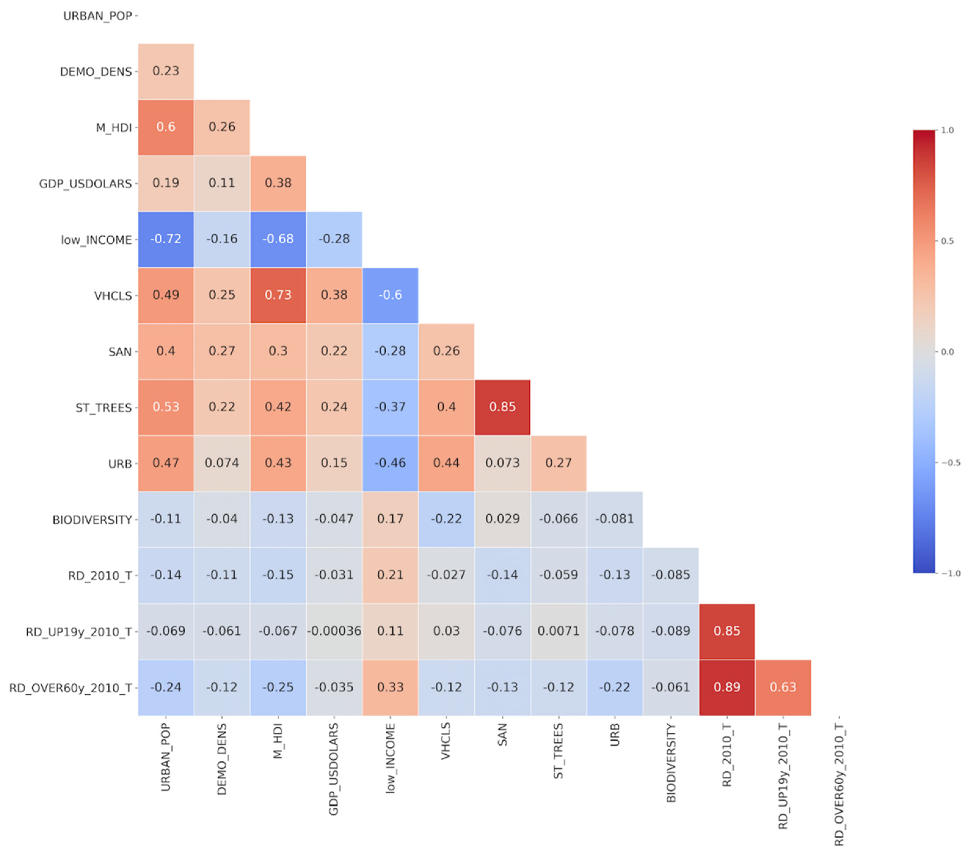
3.5. Autocorrelation Matrix

The autocorrelation matrix shows the Pearson coefficients combined two by two covering all the independent and dependent variables, revealing the degree of linear correlation among the variables (14). The closer it is to 1, the higher the correlation. In the autocorrelation matrix, the diagonal represents the correlation coefficient of the variable with itself, and is equal to 1. The sign of the Pearson coefficient is also important; it is said to be inverse when negative, indicating that an increase in one variable results in a decrease of the other. It can be represented by a right triangle, as the matrix shows symmetry. On many occasions the diagonal is suppressed, as it is all equal to 1. Although it varies according to the issue under study, a Pearson coefficient of approximately 0.60 (+/−) and above is considered a good correlation between variables. Figure 14 presents one of the autocorrelation matrixes in the form of a “heatmap”. In this case, the RD rates change for the different age groups. The values within the small squares are the Pearson correlation coefficients. A “red range scale” indicates a positive correlation, and a blue one indicates a negative correlation.

The results showed that the values of the Pearson coefficient were generally coherent. The highest values, as expected, were among the rates of hospitalizations due to respiratory diseases. Among the independent variables, the highest was 0.85 between “ST_TREES” and “SAN”. The correlation between the ratio of urban population and “low_INCOME” (poverty index) was inversely correlated (r = −0.72). Therefore, the greater the percentage of urban population, the lower the proportion of the population under extreme poverty.

Figure 15 shows the distribution of the index “low_INCOME” among the municipalities and the dots are the number of hospitalizations per 100 inhabitants. Generally, municipalities in the higher ranges of “low_INCOME”, presented larger dots (higher ranges of RD). However, it is interesting to observe the case of the municipality of Guarequeçaba—the one in the eastern region of the state, in the coast. Although, it is within the higher ranges of “low_INCOME”, it presents one of the smallest dots (lower range of RD). It can be noticed that it is the same in Figure 4, which is within the highest ranges for the “BIODIVERSITY” ratio.

Regarding the correlation of urban green spaces with RD indexes, although “URB” and “BIODIVERSITY” did not show high values for the Pearson coefficient, they were always negative. These results were consistent for all population groups. As for the poverty index, the Pearson coefficient was always positive for all population groups. Regarding the “ST_TREES” index, it was positive for the population group of up to 19 years old.

p_values, associated with the significance levels of the linear correlations, were also calculated. Most of the p_values were less than 0.05, which guarantees a good level of significance. For the variable ‘low_INCOME’, ‘p’ consistently presented low values, indicating high significance levels. Regarding ‘ST_TREES’, p_values were above 0.05 three times. For correlation with ‘RD’, ‘p’ was 0.242, and 0.887 for the population group of people with up to 19 years old. This, therefore, is indicative of, low significance, especially for the population of this group that presented positive correlation. For the variable ‘BIODIVERSITY’, the ‘p_value’ was greater than 0.05 nine times (in thirteen possible correlations). Regarding the correlations between ‘BIODIVERSITY’ and ‘RD’ (health index), ‘p’ was equal to 0.09; 0.078 and 0.222, for RD in the total population group, up to 19 years old and above 60, respectively. For the population group of up to 19 years old, the correlation with all variables presented lower levels of significance.

3.6. Cluster Analysis

A dendrogram of variables is presented in Figure 16, which was built considering the “single-linkage” method and the Euclidean distances. The most similar variables are the rates of hospitalizations, because of respiratory diseases (RD), for different population groups, which presented the least Euclidean distances.

Two distinct “branches” are observed. One branch, cluster 1, grouped the dependent variables (outputs, or the variables to be explained by the independent features)—the rates of hospitalizations because of respiratory diseases related to different population groups—and two independent variables (seen as input, the ones that would explain the dependent variables)—“low_INCOME” and “BIODIVERSITY”. The remaining independent variables were grouped in cluster 2.

Within cluster 1, another two distinct “branches” can be distinguished: in red, the one that grouped all hospitalization rates (morbidity) due to respiratory diseases, and, in blue, another, that grouped “low_INCOME” (associated with poverty) and “BIODIVERSITY” (area per person of biodiversity conservation units). Within the “red branch”, it can be observed that the RD of different age population groups was in separate clusters. And, within each of these (age population groups) clusters, were the groups by gender.

3.7. Selection of Attributes (SelectKBest)

Table 5. Independent variable scores for features selection.

Population Groups	TOT_POP	DEMO_ DENS	M_HDI	GDP_ USD	Low_ INCOME	VHCLS	SAN	ST_TREES	URB	BIODIVERSITY
All	6	4	5	10	1	9	3	8	2	7
Women	3	6	4	10	1	9	5	8	2	7
Men	6	5	4	10	1	9	2	7	3	8
All up to 19 years old	9	3	6	8	5	1	4	10	7	2
Women up to 19 years old	3	7	1	9	4	2	6	10	8	5
Men up to 19 years old	8	6	2	9	1	7	3	10	4	5
All over 60 years old	4	7	3	9	1	8	6	5	2	10
Women over 60 years old	3	8	2	9	1	5	6	7	4	10
Men over de 60 years old	4	5	3	9	1	8	6	7	2	10

Scale 1 to 10 (1: most important; 10: least important)

presents the degree of importance of the independent variables in explaining the dependent ones; “1” being the most important and “10” being the least important. The first column shows the indexes for RD for the different population groups (dependent variable) considered each time. Notably, the index related to wealth (“GDP_USD”) was consistently the least important compared to the one associated with poverty (“low_INCOME”).

By integrating all knowledge acquired from previous analyses and the study by “SelectKBest”, the attributes selected for the independent variables to be considered for associative mining rules by the CBA algorithm were URBAN_POP, DEMO_DENS, M_HDI, low_INCOME, VHCLS, SAN, ST_TREES, URB, and BIODIVERSITY. The dependent variable was the rate of hospital morbidity per 100 inhabitants due to respiratory disease (population data from the IBGE 2010 census).

3.8. Associative Rules Mining

Some of the associative rules obtained are presented in

Table 6. Associative Rules.

Rule	Logic Sentence		Support	Confidence
	IF	THEN
1	URB (high)	ST_TREES (high)	12.06	97.92
	SAN (high)
2	M_DHI (high)	ST_TREES (high)	17.839	97.18
	SAN (high)
3	SAN (low)	ST_TREES (low)	10.05	87.5
	RD_2010_T (high)
4	ST_TREES (low)	SAN (low)	9.548	92.11
	RD_2010_T (high)
5	ST_TREES (high)	SAN (high)	9.296	86.49
	RD_2010_T (medium)
6	RD_2010_T (low)	URBAN_POP (high)	4.774	100
	VHCLS (high)
	low_INCOME (low)
	BIODIVERSITY (medium)

Scale: darker to lighter color is related to the range of features. Darker is the higher range and lighter, the lower.

. Among others, these rules involve street trees (ST_TREES), biodiversity (BIODIVERSITY), and rates of hospitalizations because of respiratory diseases (RD).

In the framework for data entry in CBA, the number of rules was defined as very high in order to obtain all possible rules. Minimum support and accuracy were set as low values for the same reason. The maximum number of logic sentences in each rule was initially set to three. All the variables were previously normalized by standardization (SCIKIT-LEARN. preprocessing. StandardScaler).

Rule 2 in Table 6 interrelated M_HDI, SAN and ST_TREES, and showed very good confidence and excellent support. It also seemed to be very coherent. The rules 3, 4, and 5 interrelate health indexes (RD_2010_T), street tree index (ST_TREES), and adequate sanitation (SAN). Although accuracy and support were not as high as those of the previous rules, it is still an interesting associative rule and is also coherent.

Some rules involving the index for biodiversity conservation unit area per inhabitant (BIODIVERSITY) were also obtained, but admitted a large number of logic sentences. Though the accuracy was very high (100%), the support was not as good (4774). This is rule 6 in Table 6. Notably, the rule establishes associations among the indices for respiratory health, urban green space, sanitation, ‘vehicles per person’, poverty levels, and the urban population ratio.

4. Discussion

In this study we applied data science including a data-mining algorithm to find out if UGI could directly provide ES towards respiratory health protection in a socioeconomic scenario typical of the Global South countries. It is a cross sectional study in which multiple datasets were applied to uncover relationships and patterns.

4.1. UGI and RD

The most important finding was that vegetation (UGI) has proved to have a direct effect on diminishing hospitalization rates because of respiratory diseases (RD) in the municipalities of the state of Paraná, Brazil. This suggests that the green infrastructure provides ecosystem services towards respiratory health protection.

Two different typologies of UGI were studied. Regarding the effects in the direct relationship between vegetation and hospitalizations because of respiratory diseases (RD), the area per person of biodiversity conservation units (“BIODIVERSITY”) seemed to have a different strength than the feature associated with the urban street trees (“ST_TREES”). “ST_TREES” did not always present an inverse Pearson correlation coefficient (r) with RD (14).

No major difference was observed regarding population and age subgroups regarding UGI features and RD for municipalities with and without biodiversity conservation units (Figure 12 and Figure 13), except for women over 60 years old, for which the average rates of hospitalizations per 100 inhabitants were slightly larger for the municipalities with biodiversity areas (2010 census population data, Figure 5). The high rates of hospitalization among the elderly (population over 60 years old) and the even higher rates for the male population are noteworthy. For the analysis considering years after 2010 (Figure 6 and Figure 7), however, population figures are based in growth estimates, because there has been no population survey for all municipalities since the census survey in 2010.

In relation to municipalities’ population size and typology, we found that 56.93% of the municipalities in Paraná are of the typology adjacent to rural areas and of S_1 size (up to 20,000 inhabitants). And we argued that small municipalities surrounded by rural areas are prone to have less air pollution. However, considering both municipalities’ subgroups regarding biodiversity conservation units (with and without), most municipalities have up to 20,000 inhabitants (S_1) in both subgroups. In addition, among the municipalities without biodiversity conservation units, nearly 90% are classified as S_1. Moreover, the ten largest municipalities in terms of population (e.g., Curitiba, Londrina, Guarapuava, Paranaguá, Cascavel, and Maringá) are all included in the group of municipalities with biodiversity conservation units. We also observed in Figure 9 that in the higher range of “ST_TREES”, most of the municipalities are of the urban class, including the largest-size municipalities.

We lacked data to represent air pollution for all municipalities. However, there was no apparent reason to conclude that the municipalities without biodiversity conservation units would be more prone to air pollution issues, or that those with the biodiversity conservation units would be more likely to have fewer problems regarding air pollution.

The health benefits of exposure to biodiversity have also been discussed in previous studies in New Zealand [46] and in Australia [26]. Ref. [46] assessed the association between the natural environment and asthma in 49,956 New Zealand children born in 1998 and followed up until 2016 using routinely collected data. This study used normalized difference vegetation index (NDVI) values to account for the quantities of vegetation. They found that children who lived in greener areas were at a lower risk of asthma. However, they also perceived that not all vegetation cover was beneficial. Areas covered by gorse (Ulex europaeus) or exotic conifers, which are not native, as well as those typified as low-biodiversity, increase the risk of asthma. They postulate that exposure to the natural environment may increase microbial contact, resulting in improved immune function and the subsequent lower risk of allergic diseases.

Ref. [26] carried out a study in Australia and the results aligned with those of [46]. They carried out a spatial analysis based on Australia-wide gridded mapping datasets with a 250 m resolution. The analysis compared three socio-geographic settings (moderate majority, major cities, remote disadvantage) and used an array of environmental data, including vegetation-based variables. They showed that variables associated with the landscape’s biodiversity correlate with respiratory health. They raised the possibility of populations receiving some level of ambient beneficial or adverse immune-modulatory influence associated with different types and qualities of the environment.

In Northeast China, a study was carried out to investigate the benefits of green areas surrounding 94 schools in 7 different cities during 2012–2013, and higher greenness was associated to less asthma symptoms [47].

We also included in the analysis the number of vehicles in each municipality divided by the number of inhabitants (VHCLS), but unexpectedly, “VHCLS” was not always positively correlated to “RD” and this requires further investigation (Figure 14).

In the cluster analysis (Figure 16), two “branches” were revealed, and one of them, cluster 1, grouped together RD, the morbidity rates of respiratory diseases (the dependent variables) with “low_INCOME” and “BIODIVERSITY” (independent variables). This pattern suggests that among the independent variables, “low_INCOME” and “BIODIVERSITY” are more similar and most likely to better to explain RD (the hospital morbidity rates of respiratory diseases) than the remaining independent variables.

4.2. Socioeconomics, UGI and RD

As we were also interested in socioeconomic issues, we further explored the relationship of the socioeconomic features with RD and with the other features (including the relationships between each other). Three of the features are most associated to the socioeconomics issues: the number of households with a monthly income of up to half the Brazilian minimum salary in 2010, divided by the total households in the municipality (low_INCOME)—statistic most directly associated to poverty; the Municipal Human Developed Index (M_HDI) (In the developing world, according to UN (http://hdr.undp.org/en/content/developing-regions, (accessed on 29 December 2021), Brazil (with HDI of about 0.700) ranks 84, meanwhile Argentina and Chile rank 46 and 43 respectively, and Haiti ranks 170. China and India rank 85 and 131, respectively), which is a statistic composite index of life expectance, education and per capita income indicators; and GDP_USDOLARS, which is mostly associated with wealth and the size of different economies—it is a measure of economy size and the health of a country.

Figure 10 presents “low_INCOME” versus RD classified by the typology (a) and size (b) of the municipalities. It shows that the medium and large municipalities are in the lower range of “low_INCOME” as well as the urban type (b). At the same time, “low_INCOME” was inversely correlated to “GDP_USDOLARS” and to “M_HDI”. And, as it can be seen in Figure 11 urban type are concentrated in the higher range of “M_HDI” (a) as well as, the medium- large-sized municipalities (b). And, these (lower range of “low_INCOME” and, higher range of “M_HDI”) are all concentrated in the lower range of RD. It suggests that socioeconomic issues play an important role in lowering RD rates, and not only UGI. “low_INCOME” always showed a positive correlation with RD (Figure 14 and Figure 15) with p_values < 0.05, which guarantees high levels of significance in the linear correlations. Besides, it had lower scores (most important) in the SelectKbest analysis meanwhile “GDP_USDOLAR” had higher scores (least important) (Table 5).

Nevertheless, considering the subgroups of municipalities with (n = 195) and without (n = 202) biodiversity conservation units, the average of the feature “low_INCOME” for the S_1 municipalities (up to 20,000 inhabitants) was slightly higher for the set of municipalities with conservation units (0.035 against 0.029). It shows once more the positive effect of the biodiversity conservation units on lowering the rates of hospitalizations because of respiratory diseases (see also Figure 5, Figure 6 and Figure 7).

Apart of that, “low_INCOME” showed an inverse correlation with “URBAN_POP” (URBAN_POP always correlated inversely with “RD”, “BIODIVERSITY” and “low_INCOME”), “DEMO_DENS” (DEMO_DENS always correlated inversely with “RD”, “BIODIVERSITY” and “low_INCOME”),“VHCLS”, “ST_TREES”, “SAN” (associated with sanitation infrastructure), and “URB” (associated to the presence of curb and sidewalks). And these six features, which were positively correlated to each other, were also positively correlated with “GDP_USDOLARS” and “M_HDI”. It can also be observed in Figure 16 that these features are within the same cluster and are articulated in many of the association rules obtained by the CBA mining algorithm (Table 6). These patterns reveal environmental inequality/injustice, in which the poorer seems to be exposed to lower standards of environmental and landscape quality [48]. In this context, Ref [49] argues that socioeconomics can partly overrides and are cofounders of the UGI ecosystems services towards respiratory health.

4.3. Data Mining

Regarding the application of the data-mining CBA algorithm, we obtained coherent associative rules (Table 6). We also highlighted the contribution to the selection of features that best explain the phenomenon of UGI and respiratory health. Although the rules that linked the conservation area per inhabitant (BIODIVERSITY) and the rates of hospitalizations because of respiratory diseases presented a confidence of up to 100%, they showed lower support than those that linked street tree rates (“ST_TREES”), with confidence up to 95% and support of nearly 15%. The remainder also involved a lower number of logic sentences. We believe that the fact that the feature “BIODIVERSITY” has such a leptokurtic distribution with a null median may have impacted these outcomes, and it was difficult to obtain equivalent samples in each tertile.

Overall, these results may offer good support to the proposition of public policies towards lowering risks and increasing cities’ resilience. Those entwined issues (socioeconomic, sanitation, UGI and respiratory health) present a great opportunity; acting on them would have transversal impacts in many of the SDGs (Mainly SDG 3—good health and wellbeing, and 11—sustainable cities and communities. Moreover, they will also have transversal benefits for SDGs 6 (water and sanitation) and 13 (climate actions), as preserving and increasing vegetated spaces works towards water conservation and reducing greenhouse gases in the atmosphere).

That being said, one should always consider the possibility of hospital sub-notifications. There is also an intrinsic uncertainty in the process of acquiring and registering data, although it is unlikely to compromise the results. In addition, although Brazil has a universal health system (SUS) with a standard and relatively homogeneous service for public health care, as well as a diverse population with respect to ethnicities and races, causality should always be considered. It could be, although unlikely, a particular reason for the findings of this research, such as a specificity regarding the population of Paraná or some of its municipalities, the population pyramid, culture, behavior, inner municipality-scale, the health care system, or a combination of all these data, which could add or better explain these results.

5. Conclusions

One of the trends for urban development towards sustainability is the increase in green spaces in cities. Whether vegetation can be beneficial to respiratory health remains controversial. This study investigated if the UGI, as in nature based solutions, can or cannot directly provide ecosystem services towards respiratory health protection in the context of the socioeconomic scenario of the Global South countries. It involved a data science approach for 397 municipalities of the state of Paraná, in Brazil’s South region. The study initially involved an exploratory analysis to select the best features to study UGI—a respiratory health phenomenon. As health, socioeconomic, and environmental issues tend to be entwined, the dataset and features chosen for the study included multiple data. Overall, 15 features were chosen for the study. They were public domain data from the Brazilian census database, from the Brazilian Health Ministry, from the National Department of Transit, and from the Paraná State Institute for Water and Land. Some features were weighted by the total population and by segments related to sex and age groups. Two indices were chosen to represent UGI: one associated with street trees and another with the area of biodiversity conservation units per inhabitant within the limits of the municipality.

The results showed that the selected features to the subject were adequate and successful in representing the phenomenon. It was concluded that urban green spaces as units of conservation of biodiversity have a positive effect on respiratory diseases, as these showed an effect on reducing the hospitalization rates. Hospitalization rates because of respiratory diseases (CID-10 X) were inversely correlated to the biodiversity rates. On average, hospitalizations because of respiratory diseases were lower for the municipalities with green areas of biodiversity. The biodiversity index showed to be more closely related to the protection of respiratory health than the street tree index. The correlation matrix showed no particular pattern for the different population segments.

The cluster analysis grouped all dependent variables (respiratory disease rates for different population subgroups) and two independent variables (low_INCOME and BIODIVERSITY) in the same cluster, which means that these two independent variables were better than the others in explaining the UGI-RD phenomenon.

Regarding the socioeconomic features, the Pearson correlation coefficient between “low_INCOME” and “RD” was positive and inversely correlated to the variables associated to sanitation and urbanization features (curb, sidewalk, street trees). In these cases, the correlation coefficient was generally higher if compared with the coefficient between UGI (BIODIVERSITY and ST_TREES) and RD (hospitalizations because of respiratory diseases per 100 inhabitants), with p value below 0.05. This suggests that environmental issues and respiratory health are entwined with the socioeconomic features considered in this study.

The data mining analysis revealed interesting associative rules consistent with the learning from the basic statistics and multivariate analysis. It showed with reasonable support and confidence that sanitation, urban ordinance and the street tree index are related in the upper tertiles. Other rules revealed patterns showing that both BIOBERSITY and ST_TREES can protect respiratory health. No particular rule/pattern was identified for the population segments studied.

These results can support public policies towards environmental and health sustainable management. Lowering rates of hospitalizations due to respiratory diseases has a collateral benefit on reducing costs of hospitalizations because of health aggravations and other infections, and it can contribute towards reducing absenteeism in school and in the workplace as well.

References

1. Scott, M.; Lennon, M.; Haase, D.; Kazmierczak, A.; Clabby, G.; Beatley, T. Nature-based solutions for the contemporary city/Re-naturing the city/Reflections on urban landscapes, ecosystems services and nature-based solutions in cities/Multifunctional green infrastructure and climate change adaptation: Brownfield greening as an adaptation strategy for vulnerable communities?/Delivering green infrastructure through planning: Insights from practice in Fingal, Ireland/Planning for biophilic cities: From theory to practice. Plan. Theory Pract. 2016, 17, 267–300. [Google Scholar] [CrossRef] [Green Version]
2. Jaligot, R.; Chenal, J. Integration of ecosystem services in regional spatial plans in Western Switzerland. Sustainability 2019, 11, 313. [Google Scholar] [CrossRef] [Green Version]
3. Parker, J.; de Baro, M.E.Z. Green infrastructure in the urban environment: A systematic quantitative review. Sustainability 2019, 11, 3182. [Google Scholar] [CrossRef] [Green Version]
4. Ministry of Housing, Communities and Local Government. National Planning Policy Framework (London, England). 2021; Volume 1, pp. 1–75. Available online: www.gov.uk/government/publications (accessed on 14 October 2021).
5. Andersson-Sköld, Y.; Klingberg, J.; Gunnarsson, B.; Cullinane, K.; Gustafsson, I.; Hedblom, M.; Knez, I.; Lindberg, F.; Sang, Å.O.; Pleijel, H.; et al. A framework for assessing urban greenery’s effects and valuing its ecosystem services. J. Environ. Manag. 2018, 205, 274–285. [Google Scholar] [CrossRef]
6. Barnes-Mauthe, M.; Oleson, K.L.L.; Brander, L.M.; Zafindrasilivonona, B.; Oliver, T.A.; van Beukering, P. Social capital as an ecosystem service: Evidence from a locally managed marine area. Ecosyst. Serv. 2015, 16, 283–293. [Google Scholar] [CrossRef] [Green Version]
7. Garrigos-Simon, F.J.; Botella-Carrubi, M.D.; Gonzalez-Cruz, T.F. Social capital, human capital, and sustainability: A Bibliometric and visualization analysis. Sustainability 2018, 10, 4751. [Google Scholar] [CrossRef] [Green Version]
8. Koc, C.B.; Osmond, P.; Peters, A. Towards a comprehensive green infrastructure typology: A systematic review of approaches, methods and typologies. Urban Ecosyst. 2017, 20, 15–35. [Google Scholar] [CrossRef]
9. Fletcher, T.D.; Shuster, W.; Hunt, W.F.; Ashley, R.; Butler, D.; Arthur, S.; Trowsdale, S.; Barraud, S.; Semadeni-Davies, A.; Bertrand-Krajewski, J.-L.; et al. SUDS, LID, BMPs, WSUD and more—The evolution and application of terminology surrounding urban drainage. Urban Water J. 2015, 12, 525–542. [Google Scholar] [CrossRef]
10. Sussams, L.W.; Sheate, W.R.; Eales, R.P. Green infrastructure as a climate change adaptation policy intervention: Muddying the waters or clearing a path to a more secure future? J. Environ. Manag. 2015, 147, 184–193. [Google Scholar] [CrossRef]
11. Ferreira, J.C.; Monteiro, R.; Silva, V.R. Planning a green infrastructure network from theory to practice: The case study of Setúbal, Portugal. Sustainability 2021, 13, 8432. [Google Scholar] [CrossRef]
12. Markevych, I.; Schoierer, J.; Hartig, T.; Chudnovsky, A.; Hystad, P.; Dzhambov, A.M.; de Vries, S.; Triguero-Mas, M.; Brauer, M.; Nieuwenhuijsen, M.; et al. Exploring pathways linking greenspace to health: Theoretical and methodological guidance. Environ. Res. 2017, 158, 301–317. [Google Scholar] [CrossRef] [PubMed]
13. Suppakittpaisarn, P.; Jiang, X.; Sullivan, W.C. Green Infrastructure, Green Stormwater Infrastructure, and Human Health: A Review. Curr. Landsc. Ecol. Rep. 2017, 2, 96–110. [Google Scholar] [CrossRef] [Green Version]
14. Amato-Lourenço, L.F.; Moreira, T.C.L.; de Arantes, B.L.; Filho, D.F.d.; Mauad, T. Metrópoles, cobertura vegetal, áreas verdes e saúde. Estud. Av. 2016, 30, 113–130. [Google Scholar] [CrossRef]
15. Nowak, D.J.; Hirabayashi, S.; Doyle, M.; McGovern, M.; Pasher, J. Air pollution removal by urban forests in Canada and its effect on air quality and human health. Urban For. Urban Green. 2018, 29, 40–48. [Google Scholar] [CrossRef]
16. Moktan, S.; Rai, P. Research Article Ethnobotanical Approach Against Respiratory Related Diseases and Disorders in Darjeeling Region of Eastern Himalaya. NeBIO 2019, 10, 99–105. [Google Scholar]
17. Tai, A.; Tran, H.; Roberts, M.; Clarke, N.; Wilson, J.; Robertson, C.F. The association between childhood asthma and adult chronic obstructive pulmonary disease. Thorax 2014, 69, 805–810. [Google Scholar] [CrossRef] [Green Version]
18. Annerstedt van den Bosch, M.; Mudu, P.; Uscila, V.; Barrdahl, M.; Kulinkina, A.; Staatsen, B.; Swart, W.; Kruize, H.; Zurlyte, I.; Egorov, A.I. Development of an urban green space indicator and the public health rationale. Scand. J. Public Health 2016, 44, 159–167. [Google Scholar] [CrossRef]
19. van Dorn, A. Urban planning and respiratory health. Lancet Respir. Med. 2017, 5, 781–782. [Google Scholar] [CrossRef]
20. WHO. Urban Green Space Interventions and Health: A Review of Impacts and Effectiveness; World Health Organization: Geneva, Switzerland, 2017.
21. Schirmer, W.N.; Quadros, M.E. Compostos Orgânicos Voláteis Biogênicos Emitidos a Partir de Vegetação e Seu papel no ozônio troposférico urbano. Rev. Soc. Bras. Arborização Urbana 2010, 5, 25–42. [Google Scholar] [CrossRef]
22. Eisenman, T.S.; Churkina, G.; Jariwala, S.P.; Kumar, P.; Lovasi, G.S.; Pataki, D.E.; Weinberger, K.R.; Whitlow, T.H. Urban trees, air quality, and asthma: An interdisciplinary review. Landsc. Urban Plan. 2019, 187, 47–59. [Google Scholar] [CrossRef]
23. Russo, A.; Cirella, G.T. Modern compact cities: How much greenery do we need? Int. J. Environ. Res. Public Health 2018, 15, 2180. [Google Scholar] [CrossRef] [PubMed] [Green Version]
24. Amano, T.; Butt, I.; Peh, K.S.H. The importance of green spaces to public health: A multi-continental analysis. Ecol. Appl. 2018, 28, 1473–1480. [Google Scholar] [CrossRef] [PubMed]
25. Erdman, E.; Liss, A.; Gute, D.; Rioux, C.; Koch, M.; Naumova, E. Does the presence of vegetation affect asthma hospitalizations among the elderly? A comparison between rural, suburban, and urban areas. Int. J. Environ. Sustain. 2015, 4, 114. [Google Scholar] [CrossRef]
26. Liddicoat, C.; Bi, P.; Waycott, M.; Glover, J.; Lowe, A.J.; Weinstein, P. Landscape biodiversity correlates with respiratory health in Australia. J. Environ. Manag. 2018, 206, 113–122. [Google Scholar] [CrossRef]
27. Pimentel da Silva, L.; de Souza, F.T. Urban Management: Learning from Green Infrastructure, Socioeconomics and Health Indicators in the Municipalities of the State of Paraná, Brazil, Towards Sustainable Cities and Communities. In Universities and Sustainable Communities: Meeting the Goals of the Agenda 2030; World Sustainability Series; Leal Filho, W., Tortato, U., Frankenberger, F., Eds.; Springer: Cham, Switzerland, 2020. [Google Scholar] [CrossRef]
28. Kowarik, I. Cities and Wilderness-A New Perspective. Int. J. Wilderness Int. J. Wilderness 2013, 19, 32–36. [Google Scholar]
29. Alcock, I.; White, M.; Cherrie, M.; Wheeler, B.; Taylor, J.; McInnes, R.; Otte im Kampe, E. Land cover and air pollution are associated with asthma hospitalisations: A cross-sectional study. Environ. Int. 2017, 109, 29–41. [Google Scholar] [CrossRef]
30. Hunter, R.F.; Cleland, C.; Cleary, A.; Droomers, M.; Wheeler, B.W.; Sinnett, D.; Nieuwenhuijsen, M.J.; Braubach, M. Environmental, health, wellbeing, social and equity effects of urban green space interventions: A meta-narrative evidence synthesis. Environ. Int. 2019, 130, 104923. [Google Scholar] [CrossRef]
31. Aerts, R.; Honnay, O.; van Nieuwenhuyse, A. Biodiversity and human health: Mechanisms and evidence of the positive health effects of diversity in nature and green spaces. Br. Med. Bull. 2018, 127, 5–22. [Google Scholar] [CrossRef] [Green Version]
32. Poverty, Health, & Environment. 2008. Available online: https://www.cbd.int/financial/doc/Pov-Health-Env-CRA.pdf (accessed on 20 January 2022).
33. Braveman, P.; Gottlieb, L. The social determinants of health: It’s time to consider the causes of the causes. Public Health Rep. 2014, 129, 19–31. [Google Scholar] [CrossRef] [Green Version]
34. IBGE, Brazilian Census. 2010. Available online: https://sidra.ibge.gov.br/acervo#/S/Q (accessed on 30 December 2021).
35. Alvares, C.A.; Stape, J.L.; Sentelhas, P.C.; Gonçalves, J.L.d.; Sparovek, G. Köppen’s climate classification map for Brazil. Meteorol. Z. 2016, 22, 711–728. [Google Scholar] [CrossRef]
36. IPARDES (Parana’s Institute of Economics and Social Development). Municipality, Statistics Notebook; Curitiba Municipality: Curitiba, Brazil, 2018; 44p. Available online: http://www.ipardes.gov.br/cadernos/MontaCadPdf1.php?Municipio=80000 (accessed on 30 December 2021)Curitiba, Brazil.
37. SESA (PARANÁ). Relatório Anual de Gestão. Conselho Estadual de Saúde. Governo do Estado do Paraná. 2017; 178p. Available online: https://www.saude.pr.gov.br/Pagina/Relatorio-Anual-de-Gestao (accessed on 30 December 2021).
38. O’Neill, M.S.; McMichael, A.J.; Schwartz, J.; Wartenberg, D. Poverty, environment, and health: The role of environmental epidemiology and environmental epidemiologists. Epidemiology 2007, 18, 664–668. [Google Scholar] [CrossRef] [PubMed]
39. JHalonen, I.; Lanki, T.; Yli-Tuomi, T.; Kulmala, M.; Tiittanen, P.; Pekkanen, J. Urban air pollution, and asthma and COPD hospital emergency room visits. Thorax 2008, 63, 635–641. [Google Scholar] [CrossRef] [PubMed] [Green Version]
40. Liu, B.; Hsu, W.; Ma, Y. Integrating classification and association rule mining. In Knowledge Discovery and Data Mining; KDD’98; AAAI Press: New York, NY, USA., 1998; pp. 80–86. [Google Scholar]
41. Souza, F.T.; Rabelo, W.S. A data mining approach to study the air pollution induced by urban phenomena and the association with respiratory diseases. In Proceedings of the 2015 11th International Conference on Natural Computation (ICNC), Zhangjiajie, China, 11 August 2015. [Google Scholar] [CrossRef]
42. Cardoso, M.B.; de Souza, F.T. Prediction of hospitalizations caused by respiratory diseases by using data mining techniques: Some applications in Curitiba, Brazil and The Metropolitan Area. WIT Trans. Ecol. Environ. 2017, 211, 231–241. [Google Scholar]
43. de Souza, F.T. Morbidity Forecast in Cities: A Study of Urban Air Pollution and Respiratory Diseases in the Metropolitan Region of Curitiba, Brazil. J. Urban Health 2019, 96, 591–604. [Google Scholar] [CrossRef] [PubMed]
44. Belon, A.P.; Lima, M.G.; Barros, M.B.A. Gender differences in healthy life expectancy among Brazilian elderly. Health Qual. Life Outcomes 2014, 12, 110. [Google Scholar] [CrossRef] [PubMed] [Green Version]
45. IBGE. Classificação e Caracterização dos Espaços Rurais e Urbanos do Brasil: Uma Primeira Aproximação. Coordenação de Geografia—Rio de Janeiro. 2017; 84p. Available online: https://biblioteca.ibge.gov.br/visualizacao/livros/liv100643.pdf (accessed on 30 December 2021).
46. Donovan, G.H.; Gatziolis, D.; Longley, I.; Douwes, J. Vegetation diversity protects against childhood asthma: Results from a large New Zealand birth cohort. Nat. Plants 2018, 4, 358–364. [Google Scholar] [CrossRef] [PubMed]
47. Zeng, X.W.; Lowe, A.J.; Lodge, C.J.; Heinrich, J.; Roponen, M.; Jalava, P.; Dong, G.H. Greenness surrounding schools is associated with lower risk of asthma in schoolchildren. Environ. Int. 2020, 143, 105967. [Google Scholar] [CrossRef]
48. Shao, S.; Liu, L.; Tian, Z. Does the environmental inequality matter? A literature review. Environ. Geochem. Health 2021, 2, 124. [Google Scholar] [CrossRef]
49. Kabisch, N.; van den Bosch, M.; Lafortezza, R. The health benefits of nature-based solutions to urbanization challenges for children and the elderly—A systematic review. Environ. Res. 2017, 159, 362–373. [Google Scholar] [CrossRef]
Figure 1. The municipalities of the state of Paraná, Brazil.
Sustainability 14 01835 g001
Figure 2. Percentage of population up to 19 and over 60 years old among women and men.
Sustainability 14 01835 g002
Figure 3. Municipalities of Paraná according to their size and typology (rural-urban).
Sustainability 14 01835 g003
Figure 4. Biodiversity area (ha) per inhabitant and number of hospitalizations per 100 inhabitants in the municipalities of the state of Paraná.
Sustainability 14 01835 g004
Figure 5. Mean rates of hospital morbidity per 100 inhabitants for the municipalities with and biodiversity conservation units (2010 census population data).
Sustainability 14 01835 g005
Figure 6. Mean hospital morbidity accumulated from 2010 to 2019 per 100 inhabitants (population data from the 2010 census) for the municipalities with and without biodiversity conservation units.
Sustainability 14 01835 g006
Figure 7. Means of the rates of hospital morbidity for the period of 2010 to 2019 (estimated population for each year between 2011 and 2019 by IBGE) for the municipalities with and without biodiversity.
Sustainability 14 01835 g007
Figure 8. Scatter plots.
Sustainability 14 01835 g008
Figure 9. “ST_TREES” and “RD_2010_T” classified by rural-urban typology.
Sustainability 14 01835 g009
Figure 10. “low_INCOME” and “RD_2010_T” classified by the municipality’s size and rural-urban typology. (a) Classified by municipality’s rural-urban typology. (b) Classified by municipality’s size.
Sustainability 14 01835 g010
Figure 11. “M_HDI” and “RD_2010_T” classified by the municipality’s size and rural-urban typology. (a) Classified by municipality’s rural-urban typology. (b) Classified by municipality’s size.
Sustainability 14 01835 g011
Figure 12. Histograms for independent variables.
Sustainability 14 01835 g012
Figure 13. Histograms for dependent variables.
Sustainability 14 01835 g013
Figure 14. Autocorrelation matrix: All population and age subgroups (Autocorrelation matrix design: https://www.kdnuggets.com/2019/07/annotated-heatmaps-correlation-matrix.html. (accessed on 26 October 2020)).
Sustainability 14 01835 g014
Figure 15. Number of households with a monthly income of up to half the Brazilian minimum salary in 2010 divided by the households in the municipality (low_INCOME) and number of hospitalizations because of respiratory diseases per 100 inhabitants (RD) in the municipalities of the state of Paraná.
Sustainability 14 01835 g015
Figure 16. The dendrogram of variables.
Sustainability 14 01835 g016