Abstract
The weigh-in-motion (WIM) system is a necessary piece of equipment for an intelligent road. It can provide real-time vehicle weight and lateral distribution data on wheel load to effectively support pavement structure design and service life analysis for autonomous driving. This paper proposed an enhanced weigh-in-motion sensors system using Fabry–Pérot (F-P) cavity fiber optical technology. Laboratory testing was performed to evaluate the feasibility of the proposed system and field application was conducted as well. The laboratory results show that the traffic loads could be obtained by measuring the center wavelength changes in the embedded F-P Cavity tunable filter. The laboratory results also show that the vehicle load and the number of vehicle axles can be estimated based on the system transfer function between the dynamic loading and the wavelength variation. The field application indicates that the weighting accuracy of the proposed system could reach 94.46% for moving vehicles, and the vehicle passing speed is the potentially relevant factor. The proposed system also has the ability to estimate the number of vehicle axles and the loading position, and the precision could reach 97.1% and 300 mm, respectively.
1. Introduction
Estimation of vehicle weight and lateral distribution of wheel is a controlling factor in durable pavement structure design for autonomous driving, which significantly affects the pavement’s maintenance costs and the safety of road users [1,2]. The weigh-in-motion (WIM) method may directly identify the load characteristic when the vehicles are in motion. Weigh-in-motion (WIM) is also commonly used in vehicle overload controls and charge freeway tolls [3,4,5]. In freeway management, it is indispensable to guarantee the qualified performance of transportation infrastructure regarding traffic variations according to weather factors [6,7], and determine the freeway toll for each vehicle.
Traditional WIM sensors usually include load cells, bending plate and strip sensors. The bending plate and load cells have a metal plate several strain gauges beneath them, to acquire the vehicle load by measuring the deformation of the metal plate. However, this type of WIM sensor requires the vehicle to pass the metal plate with a low operating speed, between 5 km/h and 15 km/h, to accurately determine axle loads [8,9,10,11]. The strip sensor was first proposed in the 1980s for a high-speed WIM. Its main feature is a narrow strip with a cross-sectional width of within a few centimeters. There have been various types of bar sensor to date, including piezo-ceramics, piezo-polymer and piezo-quartz [12,13,14,15]. Alavi made a simple WIM sensor using piezoelectric ceramics. The sensor had a good performance in both cement concrete pavement and asphalt concrete pavement after the field control test of 183000 ESALs [16]. Song made embedded piezoelectric ceramic sensors based on 3D printing technology and proved their potential in vehicle weighing applications [17]. Xiong designed a WIM prototype system, composed of nine piezoelectric ceramic plates, and demonstrated that it was more reliable and cheaper than Kistler’s existing WIM products [18]. Jian used piezoelectric ceramics, piezoelectric polymers, and piezoelectric quartz sensors to fabricate a bridge WIM system and measured the instantaneous load applied by vehicle tires [19]. However, the behavior and response of the piezoelectric sensor depends on the pavement and bearing structure characteristics (above all, its modulus). Electromagnetic interference (EMI) and moisture will also cause the sensor to have a short lifecycle, with moderate error. Therefore, the piezoelectric sensor is more sensitive to its environment and conditions of use [20,21,22,23,24]. Fiber optic sensors can effectively solve the above problems compared with existing sensing technologies. Optical fiber sensors have the unique advantages of a small size, light weight, high sensitivity, and strong anti-electromagnetic interference. Additionally, fiber optic sensors have a high reliability and accuracy, making them suitable for harsh environments, such as those with a high temperature, corrosion and humidity [25,26]. At present, two main types of optical fiber sensor are used in WIM technology: fiber grating sensors and F-P Cavity fiber sensors. Malla et al. developed a special fiber optical sensor, based on measurements of optical loss under mechanical stress when making WIM sensors [27]. Myra Lydon et al. developed an all-fiber bridge WIM system and installed it on a beam-slab bridge for accurate axial load detection [24].
Many researchers have discussed the assembling and structure of optical fiber sensors using optical fiber WIM technology in the last two decades [28]. The mechanical properties, dimensions of the packaging structure, distance between the sensor and type of optical fiber used for sensor inscription will affect the final result. Investigating the response of fiber optic sensors with package structure under complex dynamic loads and establishing the mechanical response model of the package structure can help optimize the vehicle weight estimation algorithms to improve the performance of the WIM system [29].
This paper proposes an embedded hydraulic F-P cavity WIM system, which is designed to provide a low-cost and high-accuracy solution to existing WIM systems. The system uses the F-P cavity tunable filter structure embedded in the vertical hydraulic cylinder as a sensor unit. A single sensor contains four units to calculate the vehicle’s dynamic load and wheel position. The performance of the system, including accuracy and temperature compensation under different vehicles loads in motion, wheel positions, speed and temperature, was evaluated by laboratory and field tests. Through laboratory experiments, the system was tested under linear loading, sinusoidal loading, and different temperatures. Finally, the sensor was installed in a road and loaded by different vehicles. The results proved that the proposed system was a promising, low-cost, reliable and practical alternative to current WIM systems.
2. Operational Principle and Sensor Design
2.1. Principle of F-P Cavity Tunable Filter
The structure of the F-P cavity tunable filter (Figure 1c) is based on Micro-Electromechanical Systems (MEMS) technology. The principle of sensing is that the diaphragm is deformed due to the medium pressure, resulting in changes in the length of the cavity, which lead to changes in the optical path difference, which affect the light intensity in the optical fiber. According to the multibeam interference theory, the F-P cavity interference light intensity is given by Equation (1).
where I0 is the incident light intensity (cd); Ir is reflected interference light intensity (cd); R is reflectivity; L is cavity pitch (m); and λ is the incident wavelength (m).
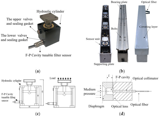
Figure 1.
Operational principle and sensor design: (a) sensor unit; (b) sensor package structure; (c) sensor unit principle; (d) F-P cavity tunable filter principle.
The light intensity can be converted into the corresponding light wavelength. Thus, the change in wavelenth can reflect the change in physical medium pressure.
Equation (2) shows the relationship between medium pressure P and wavelength variation Δw in the F-P cavity tunable filter structure medium in this article, according to the results of the laboratory calibration test.
The cantilever beam structure is used to isolate the F-P interference cavity from the air, improving its thermal isolating ability and reducing energy consumption [30].
2.2. Sensor Unit Design
The weigh-in-motion sensors sustain the complex forces formed by the interaction between the vehicle and the road [31,32]. In order to ensure the measurement accuracy and service life of the sensor, the sensor design has three principles. First, the sensor unit should have shock resistance as the support structure of the weigh-in-motion sensors. Second, the elastic deformation of the sensor unit under impact should be as small as possible in order to coordinate with the deformation of the surrounding road surface. Finally, the sensor unit should be able to measure vertical forces exclusively, which means reducing the influence of orthogonal forces on the dynamic response to improve sensing accuracy. Figure 1c shows the sensor unit in which the size of vertical hydraulic cylinder is 80 × 80 × 80 mm and the size of the internal F-P cavity tunable filter is 10 mm in diameter and 30 mm in length.
The principle of the sensor unit is based the dynamics of the cylinder. Considering the oil compressibility and cylinder leakage, the formulae of oil continuity and piston force balance can be written as Equations (3) and (4), respectively,
where A is sensor unit piston area (m2); v is sensor unit piston moving speed (m/s); κ is the leakage constant; P is the internal pressure of the cylinder (Pa); VdP/Kdt is volume change rate due to oil compression, V is the volume in the cylinder, and K is the oil elastic modulus (Pa); PA is reverse thrust of sensor unit (N); and mdv/dt is inertial force (N); B is viscous damping coefficient (N/(m/s)).
Laplacian transformation of Equations (3) and (4) is obtained:
Equations (7) and (8) are obtained from Equations (5) and (6):
when the load of sensor unit F is used as the input, the piston transfer speed v and internal pressure P are used as the output transfer functions:
where Wn is the natural angular frequency of sensor unit, and ζ is sensor unit damping ratio.
From Equations (9) and (10), it can be seen that the sensor unit can be simplified into a second-order system. Since the coefficients of the characteristic equations are all positive numbers, the sensor unit can work stably. From the analysis of natural angular frequency and damping ratio of the hydraulic cylinder, it is necessary to increase cylinder size and oil elastic modulus to reduce the dynamic error and expand the frequency response range. The size of the cylinder block could not be changed due to engineering and mechanical response limitations, so the oil elastic modulus was adjusted to increase the natural angular frequency of the sensor unit. In this paper, anti-wear hydraulic oil #46 was selected, and air in the cylinder was eliminated as much as possible during the oil injection process. The parameters of the cylinder structure system are shown in Equation (13).
2.3. Package Structure Design
In order to protect the F-P cavity tunable filter [33] and improve the accuracy of measurement, a strip-shaped array containing four sensor units was designed. The package was made of SUS304 material, which is one of the most widely used versions of stainless steel and is made up of 18% Cr (Chromium) and 8% Ni (Nickel). The package can provide enough protection for the sensor unit. The overall package structure consist of four parts: the supporting plate, the sensor unit with optical fiber, the bearing plate, and the covering layer, as shown in Figure 1b. The two bearing plates are assembled next to each other and can work independently. Under each bearing plate, the two sensor units should work synchronously. The external force exerted on sensor units should be exclusively vertical. The bearing plate should be wider than a tire, with a width that usually ranges from 175 to 335 mm. The spacing between sensor units should ensure that the vertical stress distribution on the bearing plate is even enough. Considering both the structure stability under overload and the suitable size of sensor units, the overall size of the whole system was designated as 1200 mm × 100 mm × 100 mm (Length × Width × Height). Additionally, the length of a single bearing plate was 300 mm, and the sensor units were arranged every 600 mm.
The WIM sensor is manufactured via the following steps: (1) the upper and lower valves of the cylinder are both filled with anti-wear hydraulic oil #46, and the inner air is exhausted; (2) sealing gaskets are installed at the upper and lower valves of the cylinder and F-P cavity, and the adjustable filter is installed into the cylinder from the lower valve; (3) the antiwear hydraulic oil #46 is injected into the cylinder via these valves, until the inner pressure reaches 10 MPa; (4) the sensor units are installed on the corresponding positions on the base board, and the bearing board is horizontally installed; (5) the covering layer is installed after the bolts are tightened on both bearing boards.
3. Laboratory Testing and Evaluation
3.1. Experiment Arrangement
The dynamic load of a vehicle can be converted to a semi-sine pulse load with an amplitude P and a period T [8]. As the width of the sensor is less than the length of wheel paths, the WIM sensor senses a sequence of the vehicle’s dynamic load. The tire loading process on the sensor is as shown in Figure 2a.
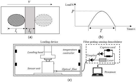
Figure 2.
Laboratory experiment design: (a) tire-loading process; (b) dynamic loading curve; (c) experiment system.
The frequency of tire loading on the sensor is calculated as follows:
where T is load period (s); v is vehicle speed (m/s); l1 is tire ground length (m); and l2 is sensor width (m).
The dynamic response and sampling frequency of the sensor significantlly affect the accuracy of the wheel load calculation. Therefore, it is necessary to consider whether the static sensing accuracy and the dynamic response frequency can both meet the requirements. As sensor units are temperature-sensitive, it is also necessary to evaluate how the sensor unit is affected by temperature. In this article, static loading and dynamic loading and temperature calibration experiments were carried out to analyze this.
A seam motion simulation servo machine was adopted in the experiment, with a maximum load of 50 kN. A loading head was used to apply a vertical force, and the loading head area is a circle, with a diameter of 100 mm. The adjustable temperature range of the servo machine was −10~50 °C. The optical fiber was connected to the FT310 optical fiber grating sensing demodulator manufactured by Shanghai BAIANTEK Sensor Technology Co., Ltd. (Shanghai, China). The optical wavelength signal was transmitted using TCP/IP. Then, the decoded data was transmitted to the HP computer for further analysis and processing. The experimental system is as shown in Figure 2c.
3.2. Loading Experiment
The loading experiment includes two parts: static loading and dynamic loading. The purpose of the static loading test is to verify the linearity of sensor units. The purpose of dynamic loading is to verify the dynamic response capability of sensor units. According to China’s Road Vehicle Outline Dimensions, Axle Loads and Mass Limits and loading capacity of the testing device, static loading stepwise was set as 10, 20, 30, and 40 kN, at the loading rate of 1 kN/s, and each loading stage was maintained for 5 s. The process was unloaded step by step after the end of loading. From Figure 2b and Equation (13), the vehicle load frequency was related to the tire-pavement contact length. Contact length was usually between 0.22 m and 0.24 m. The average value (0.23 m) was set as 11, and l2 was set as 0.1 m. Equivalent vehicle speed was 6.6 m/s. Based on the performance of the loading device, the design dynamic loading test was as a semi-sine loading sequence with the frequency of 20 Hz, and the amplitude ranged from 3 kN to 5 kN. The loading interval was 0.3 s. The experimental temperature was 25 °C.
3.3. Temperature Experiment
The sensors were generally installed on the pavement. The pavement temperature is a significant factor affecting sensor accuracy. A temperature calibration experiment was carried out to evaluate the temperature effect, by placing the sensor unit in a temperature-regulated room and measuring the change in the wavelength of sensor units at different temperatures (0, 10, 20, 40, and 60 °C).
3.4. Results and Evaluation
In the static loading experiment, when the cyclic loading of 10, 20, 30, 40 kN was exerted, the sensor unit generated a series of optical signals, which were collected by a fiber demodulator and displayed on a laptop computer. Moreover, changes in light wavelength reflected load variation.
Table 1 shows that when the wheel weight is 160 kN, the maximum vertical displacement of the cover plate is 0.24 mm less than general asphalt pavement deflection, which is approximately 0.28 mm under the same load [34]. These mean that when vehicle wheel passes over the WIM sensor, the cover plate of the sensor is elevated above the pavement level.

Table 1.
Number of different vehicle parameters (Vertical Displacement).
Figure 3a shows the cyclic loading results of the sensor unit. The repeatability and linearity of sensor units in the loading direction were well within 10–40 kN, and R2 was 0.95. This proves that a sensor proposed can measure at least the wheel weight of 160 kN (16 t).
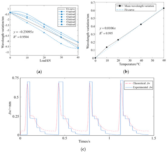
Figure 3.
Sensor unit signal at laboratory experiment: (a) static loading signal; (b) temperature calibration curve; (c) comparison between theoretical and experimental signal.
The wavelength signal measured at 0 °C was set as the control value, and the measured value of the sensor unit wavelength was subtracted from the reference value to obtain Δw. The experimental results are as shown in Figure 3b. It is clear that Δw has a remarkable linear relationship with temperature, and the temperature coefficient (0.0106 nm/°C) was obtained via linear regression.
The dynamic loading characteristics are as shown in Figure 3c. It can be seen that the sensor unit can effectively capture the changes in the loading curve. It exhibited a high response performance. According to the transfer function of the sensor unit system (Equation (10)), the response curve of the sensor under the 3 kN load with the loading frequency of 20 Hz was obtained. The comparison between theoretical and experimental results of sensor units is as shown. The actual Δw change response of the sensor unit was 92.3% of the theoretical response, which reflected the actual weighing accuracy of wheel load. In the experiment, the optical signal passed through the lowpass filter and then entered the display device, resulting in the stepped experimental response. Based on the aforementioned analysis, the actual response of the sensor unit can be corrected according to the theoretical response.
4. Field Application
4.1. Field Testing Setup
The WIM sensors were installed in two lanes of the Wutai–Yuxian Expressway in Shanxi Province for field testing. There was a static weighing station (ASTM) about 4 km downstream of the system, as shown in Figure 4a, so the license plate number, the actual vehicle weight, and the vehicle type could be known and the accuracy of the system could be calculated.
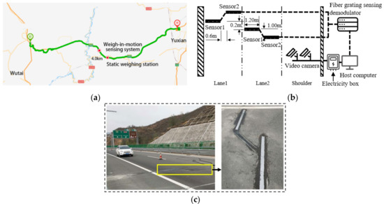
Figure 4.
Field testing setup and WIM sensor installation: (a) location of the field testing; (b) components and connections of weigh-in-motion system; (c) scene after construction and sensor installation.
In each lane, two WIM sensors were installed beneath the wheel path on the asphalt pavement. The sensor was embedded in the grooves approximately 11 cm deep, leveled with the pavement’s surface. The grooves were sealed with fast-setting epoxy (sensors almost flushed with the surface because sensor height was 10 cm). The pavement surface after construction and sensor installation is shown in Figure 4b,c. As shown in Figure 4b, the field test consisted of vehicles, a sensor embedded in the road, fiber grating sensing demodulator, video camera and host computer. The two sensors in a lane were spaced 60 cm apart.
4.2. Field Testing Data Acquisition
The field test was carried out on the 17 and 18 November 2021, and 21 December. In these three days, 153 vehicles passed the WIM sensors embedded in the pavement. These vehicles can be classified into several categories: passenger vehicles, two-axle rigid trucks, multi-axle rigid trucks, and trailers. The latter three types are freight vehicles. The number and proportion of each vehicle type were as shown in Table 2. For each vehicle passing the sensors, the video camera captured license plate number, speed and position of the vehicles. The sensors recorded signals at the same time. Every sensor unit corresponded with one channel of the demodulator. Then, signals of all the channels were demodulated in the fiber grating sensing demodulator and transmitted to the host computer. On the host computer, vehicle loads could be calculated and matched with the license plate number obtained by video camera.
Table 2.
Number of different vehicle parameters (Speed Partition).
4.3. Field Load Estimation Algorithm
To calculate vehicle loads according to the signals of the sensor, the following weigh-in-motion algorithm was proposed.
Step 1: Convert the wavelength representing hydraulic pressure to that representing force according to Equation (6). According to the Section Laboratory Experiment Results, the actual response of the sensor unit can be corrected according to the theoretical response.
Step 2: Calculate the average output wavelength. Each sensor unit outputs an array of the wavelength. The results of four sensor units are averaged, and a new array w(t) can be obtained from Equation (15).
where wi(t) (i = 1, 2, 3, 4) is the wavelength signal captured by the four sensor units during the experiment (mm); and w(t) is the average of the results of the four sensor units (mm).
Step 3: Calculate the deviation from the mean. The mean and variance of the new array are calculated and named and σ, which are two certain values. w(t) minus is adjusted to ∆w(t), as shown in Equation (16).
where is the mean of w (mm); σ is the variance in w (mm); and N is the number of wavelength samples during the experiment.
Step 4: Zero setting by three standard deviation criterions. Check for elements in the array ∆w(t), and set the elements in the range of [−3σ, 3σ] to 0. Then, the non-zero elements can be reserved as the loading response, which corresponds to a period in which a certain axle passes the sensor system.
Step5: Obtain the axial number and axle load. The integrating range is determined by the corresponding time of 5% of peak time, as shown in Figure 5a. the number of integrating ranges is exactly the axle number. As Equation (17) shows, the axial load can be obtained by integrating the axial load response during the period when ∆w ≠ 0.
where −1.6090 = 1/(−0.6215) is the coefficient of , −0.6215 is the coefficient in Equation (2); tbegin is the left-side time of the integrating range; and tend is the right-side time of the integrating range.
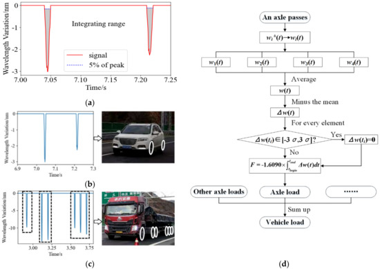
Figure 5.
The performance and flow of the WIM algorithm: (a) signal of weigh-in-motion; (b) two-axle passenger vehicle signal and scene; (c) six-axle signal and scene; (d) weigh-in-motion algorithm.
Step6: Vehicle load. The vehicle load is a simple sum of all the axial loads. The flow of the algorithm is as shown in Figure 5d.
The primary performance of the algorithm is verified in field testing. The typical traces measured by using the proposed WIM sensor and algorithm are as shown in Figure 5a (average wavelength of four sensor units). The passage of two axles can be observed, with an interval of about 0.170 s. The wheelbase calculated from speed (measured by a ra-dar speed indicator) and time intervals is 2.73 m, while the actual wheelbase of vehicle is 2.65 m. The calculation error is 3%. The wavelength variation in two types of vehicles is shown in Figure 5b. In Figure 5b, there are two integrating ranges that correspond to two axles of a passenger vehicle. Similarly, in Figure 5c, six integrating ranges are matched with the six axles. The integrating ranges can be divided into three groups, as the boxes show, which represent Single Axle, Tandem Axles and Tridem Axles, respectively. These prove that the algorithm can accurately grab the vehicle axles’ signal segment.
4.4. Field Testing Results
Data from all 153 vehicles passes are analyzed to evaluate the measurement accuracy of the vehicles’ weight and axle number. Figure 6a compares the vehicle weights estimated by the proposed WIM sensor with their actual weights. The measurement weights track the actual weights very closely, with linear correlation reaching 0.97. The means and standard deviations associated with the measurement accuracy of the vehicles’ weight and axle numbers are summarized in Table 3.
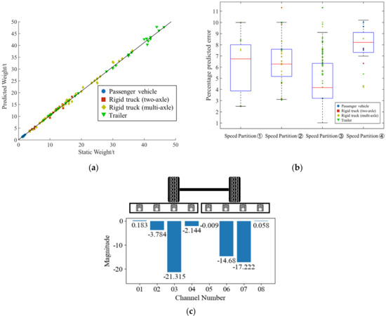
Figure 6.
Weight estimation and position estimation: (a) predicted weights against the actual static weight; (b) predicted weight percentage error of predicted weight; (c) position of the tires.
Table 3.
Results of field testing.
Figure 6b shows the percentage mean errors of different type vehicles’ weight estimates at a different speed. The error distribution is correlated with the speed. The errors of speed partition ④ and ① are larger than the others. The reason for this is that, under high speed, the greater the speed is, the greater the dynamic load factor. The WIM algorithm calculates the axle weight by integration: the slower the speed is, the more overlapped the areas. When the speed is at 60~90 km/h, the superimposed effect is balanced. This is why the error is minimal at this speed partition.
The weighing accuracy of the sensor is different for various types of vehicles, as Figure 6b shows. The more axles, the smaller the error standard deviation. This means that the consistency of heavy vehicle measurement is better than that for light vehicles.
The results of vehicle weighing and axle number detection are shown in Table 3. The accuracy of the axle number is 97.1%, while the average accuracy of axle load weighing is 94.46%. The sensor has a weighing measurement error of 7.12%, 5.94%, 5.15%, 3.47% at passenger vehicle, rigid truck (two-axle), rigid truck (multi-axle), and trailer, respectively. The error of weighing decreases with the increase in axle load. The WIM errors for the vehicle weights are below the LTPP-allowed errors (10%) [35,36].
The Table 4 shows that the proposed system has advantages in terms of the system cost of the sensor, labor cost of the system and error of WIM [29,36].
Table 4.
WIM sensor comparation.
Moreover, wheel load position can be found by comparing the signals of four channels of a sensor. When an axle of a vehicle passes, the change in wavelength can reflect the position of the tires. Channel 01~04 are in sensor 1 and the other channels are in sensor 2. As Figure 6c shows, there is significant variation in the wavelength of Channels 03, 06 and 07. This means that the left tire passed exactly on Channel 03, while the right tire passes on the middle of Channels 06 and 07. Therefore, the precision of the location of loading position reached 300 mm.
5. Conclusions
Weigh-in-motion (WIM) is an indispensable part of freeway management regarding vehicle overload controls and charge freeway tolls in China.
In this paper, an embedded hydraulic F-P cavity WIM system is designed and fabricated. After theoretical analysis, laboratory experiment and field application, the following conclusions are obtained:
- (1)
- The sensor consisting of several sensor units can measure the vertical load from 0 to 160 kN. The linear correlation coefficient of the measured value is 93.32%. The sensor has a linear relationship with temperature changes and the coefficient is 99.5%, so temperature errors can be effectively avoided through temperature compensation.
- (2)
- Field application validates that the sensor has a weighing measurement error of 5.54% and an axis number measurement accuracy of 97.1%. The speed affects the measurement accuracy, but the influence can be ignored.
- (3)
- Field application shows that the output of each sensor unit decreases as the distance from the loading center increases. According to the comparison of the output of different sensor units, the location detection resolution is 300 mm.
Further study of the temperature correction for the weighing algorithm is recommended. Moreover, further field applications are recommended to verify its feasibility under complex conditions. The new WIM system, upgrading the embedded hydraulic F-P cavity WIM system proposed in this study, could be studied in the future.
Author Contributions
Conceptualization, C.Z. and Z.B.; methodology, C.Z. and Z.B.; validation, C.Z. and Z.B.; investigation, C.Z. and Z.B.; resources, C.Z. and Z.B.; data curation, C.Z. and Z.B.; writing—original draft preparation, C.Z. and Z.B.; writing—review and editing, C.Z., Z.B., H.Z., L.M., M.G., K.P. and E.G.; visualization, C.Z. and Z.B.; supervision, C.Z. and Z.B.; project administration, C.Z. and Z.B.; funding acquisition, C.Z. and Z.B. All authors have read and agreed to the published version of the manuscript.
Funding
This work was supported by the National Natural Science Foundation of China (Grant No. 51778477 and Grant No. 51978520).
Data Availability Statement
The data presented in this study are available on request from the corresponding author.
Acknowledgments
The authors thank the editor and anonymous reviewers for their numerous constructive comments and encouragement, which have improved our paper greatly.
Conflicts of Interest
The authors declare no conflict of interest.
References
- Chen, F.; Song, M.; Ma, X. A lateral control scheme of autonomous vehicles considering pavement sustainability. J. Clean. Prod. 2020, 256, 120669. [Google Scholar] [CrossRef]
- Meyer, G.; Beiker, S. Road Vehicle Automation 5; Springer: Berlin/Heidelberg, Germany, 2019; ISBN 978-3-319-94895-9. [Google Scholar]
- Kilburn, P. Alberta Infrastructure & Transportation Weigh in Motion Report; Alberta Transportation: Admonton, AL, USA, 2005. [Google Scholar]
- Wyman, J.; Braley, G.; Stevens, R. Field Evaluation of FHWA Vehicle Classification Categories—MDOT. Executive summary. In States’ Successful Practices Weigh-In-Motion Handbook 1984; McCall, B., Vodrazka, W.C., Jr., Eds.; Federal Highway Administration: Washington, DC, USA, 1997. [Google Scholar]
- Roh, H.-J. Spatial Transferability Testing of Dummy Variable Winter Weather Model Using Traffic Data Collected from Five Geographically Dispersed Weigh-in-Motion Sites in Alberta Highway Systems. J. Transp. Eng. Part A Syst. 2020, 146, 04020128. [Google Scholar] [CrossRef]
- Roh, H.-J. Developing Cold Region Winter Weather Traffic Models and Testing Their Temporal Transferability and Model Specification. J. Cold Reg. Eng. 2019, 33, 04019009. [Google Scholar] [CrossRef]
- Ferguson, A. Weighing vehicles in motion. Meas. Control. 1969, 2, T214–T222. [Google Scholar] [CrossRef]
- Koniditsiotis, C. Weigh-in-Motion Technology; Austroads Incorporated: Sydney, Australia, 2000. [Google Scholar]
- Jia, Z.; Fu, K.; Lin, M. Tire-Pavement Contact-Aware Weight Estimation for Multi-Sensor WIM Systems. Sensors 2019, 19, 2027. [Google Scholar] [CrossRef]
- Ali, N.; Trogdon, J.; Bergan, A.T. Evaluation of piezoelectric weigh-in-motion system. Can. J. Civ. Eng. 1994, 21, 156–160. [Google Scholar] [CrossRef]
- Cheng, L.; Zhang, H.; Li, Q. Design of a Capacitive Flexible Weighing Sensor for Vehicle WIM System. Sensors 2007, 7, 1530–1544. [Google Scholar] [CrossRef]
- Richardson, J.; Jones, S.; Brown, A.; Hajializadeh, D.; Obrien, E.J. On the use of bridge weigh-in-motion for overweight truck enforcement. Int. J. Heavy Veh. Syst. 2014, 21, 83. [Google Scholar] [CrossRef]
- Zhang, W.; Li, C.-L.; Di, X.-F.; Chen, M.; Tao, S. Research on Automotive Dynamic Weighing Method Based on Piezoelectric Sensor. MATEC Web Conf. 2017, 139, 203. [Google Scholar] [CrossRef]
- Zhao, Q.; Wang, L.; Zhao, K.; Yang, H. Development of a Novel Piezoelectric Sensing System for Pavement Dynamic Load Identification. Sensors 2019, 19, 4668. [Google Scholar] [CrossRef]
- Alavi, S.H.; Mactutis, J.A.; Gibson, S.D.; Papagiannakis, A.T.; Reynaud, D. Performance Evaluation of Piezoelectric Weigh-in-Motion Sensors under Controlled Field-Loading Conditions. Transp. Res. Rec. J. Transp. Res. Board 2001, 1769, 95–102. [Google Scholar] [CrossRef]
- Song, S.; Hou, Y.; Guo, M.; Wang, L.; Tong, X.; Wu, J. An investigation on the aggregate-shape embedded piezoelectric sensor for civil infrastructure health monitoring. Constr. Build. Mater. 2016, 131, 57–65. [Google Scholar] [CrossRef]
- Xiong, H.; Zhang, Y. Feasibility Study for Using Piezoelectric-Based Weigh-In-Motion (WIM) System on Public Roadway. Appl. Sci. 2019, 9, 3098. [Google Scholar] [CrossRef]
- Jiang, X.; Vaziri, S.H.; Haas, C.; Rothenburg, L.; Kennepohl, G.; Haas, R. Improvements in piezoelectric sensors and WIM data collection technology. In Proceedings of the 2009 Annual Conference of the Transportation Association of Canada, Vancouver, BC, Canada, 18–21 October 2009. [Google Scholar]
- Burnos, P.; Gajda, J. Thermal Property Analysis of Axle Load Sensors for Weighing Vehicles in Weigh-in-Motion System. Sensors 2016, 16, 2143. [Google Scholar] [CrossRef] [PubMed]
- Liu, P.; Zhao, Q.; Yang, H.; Wang, D.; Oeser, M.; Wang, L.; Tan, Y. Numerical Study on Influence of Piezoelectric Energy Harvester on Asphalt Pavement Structural Responses. J. Mater. Civ. Eng. 2019, 31, 04019008. [Google Scholar] [CrossRef]
- Xiang, T.; Huang, K.; Zhang, H.; Zhang, Y.; Zhang, Y.; Zhou, Y. Detection of Moving Load on Pavement Using Piezoelectric Sensors. Sensors 2020, 20, 2366. [Google Scholar] [CrossRef]
- Jacob, B.; Cottineau, L.-M. Weigh-in-motion for Direct Enforcement of Overloaded Commercial Vehicles. Transp. Res. Procedia 2016, 14, 1413–1422. [Google Scholar] [CrossRef]
- Lydon, M.; Robinson, D.; Taylor, S.E.; Amato, G.; O Brien, E.J.; Uddin, N. Improved axle detection for bridge weigh-in-motion systems using fiber optic sensors. J. Civ. Struct. Heal. Monit. 2017, 7, 325–332. [Google Scholar] [CrossRef]
- Berardis, S.; Caponero, M.A.; Felli, F.; Rocco, F. Use of FBG sensors for weigh in motion. In Proceedings of the 17th International Conference on Optical Fibre Sensors, Bruges, Belgium, 23–27 May 2005; pp. 695–698. [Google Scholar]
- Zahid, M.N.; Jiang, J.; Rizvi, S. Reflectometric and interferometric fiber optic sensor’s principles and applications. Front. Optoelectron. 2019, 12, 215–226. [Google Scholar] [CrossRef]
- Malla, R.B.; Sen, A.; Garrick, N.W. A Special Fiber Optic Sensor for Measuring Wheel Loads of Vehicles on Highways. Sensors 2008, 8, 2551–2568. [Google Scholar] [CrossRef]
- Yuksel, K.; Kinet, D.; Chah, K.; Caucheteur, C. Implementation of a Mobile Platform Based on Fiber Bragg Grating Sensors for Automotive Traffic Monitoring. Sensors 2020, 20, 1567. [Google Scholar] [CrossRef] [PubMed]
- Al-Tarawneh, M.; Huang, Y.; Lu, P.; Bridgelall, R. Weigh-In-Motion System in Flexible Pavements Using Fiber Bragg Grating Sensors Part A: Concept. IEEE Trans. Intell. Transp. Syst. 2019, 21, 5136–5147. [Google Scholar] [CrossRef]
- Ou, Y.; Cui, F.; Sun, Y. Tunable Filter with Micromachine F-P Cavity on the Silicon. Opt. Des. Test. 2002, 4927, 857–863. [Google Scholar] [CrossRef]
- Hou, W.-T.; Zhao, X. Response analysis of saturated asphalt pavement under action of moving load. Highw. Eng. 2012, 21, 12–15. [Google Scholar]
- Li, H. Dynamics of Pavement Structure Under the Interaction of Vehicles and Pavement; Beijing Jiaotong University: Beijing, China, 2011. [Google Scholar]
- Dong, Z.; Tan, Y.; Ou, J. Dynamic response analysis of asphalt pavement under three-directional nonuniform moving load. China Civ. Eng. J. 2013, 46, 122–130. [Google Scholar]
- Sun, J.S.; Xiao, T.; Yang, C.F.; Sun, J.C. Study on the Axle Load Conversion Formula for Asphalt Pavement Based on Actually Measured Deflection Equivalent. In Proceedings of the International Conference on Civil Engineering and Transportation (ICCET 2011), Jinan, China, 14–16 October 2011; p. 271. [Google Scholar]
- Chatterjee, I.; Liao, C.-F.; Davis, G.A. A statistical process control approach using cumulative sum control chart analysis for traffic data quality verification and sensor calibration for weigh-in-motion systems. J. Intell. Transp. Syst. 2016, 21, 111–122. [Google Scholar] [CrossRef]
- Mitchell, M.R.; Link, R.E.; Papagiannakis, A.T. High Speed Weigh-in-Motion Calibration Practices. J. Test. Eval. 2010, 38, 1–21. [Google Scholar] [CrossRef]
- Bajwa, R.; Coleri, E.; Rajagopal, R.; Varaiya, P.; Flores, C. Development of a cost-effective wireless vibration Weigh-in-motion system to estimate axle weights of trucks. Comput. Aided Civ. Infrastruct. Eng. 2017, 32, 443–457. [Google Scholar] [CrossRef]


Publisher’s Note: MDPI stays neutral with regard to jurisdictional claims in published maps and institutional affiliations. |
© 2022 by the authors. Licensee MDPI, Basel, Switzerland. This article is an open access article distributed under the terms and conditions of the Creative Commons Attribution (CC BY) license (https://creativecommons.org/licenses/by/4.0/).