Abstract
Stormwater pipe infrastructure is a fundamental requirement of any nation, but pipes can be damaged in natural disasters. Consequently, evaluating the resilience of stormwater infrastructure to earthquake damage is an essential duty for any city because it outlines the capability to recover from a disaster after the event. The resilience quantification process needs various data types from various sources, and uncertainty and partial data may be included. This study recommends a resilience assessment framework for stormwater pipe infrastructure facing earthquake hazards using Hierarchical Evidential Reasoning (HER) on the basis of the Dempster–Shafer (D-S) theory. The developed framework was implemented in the City of Regina, SK, Canada to quantify the resilience of the stormwater pipe infrastructure. First, various resilience factors were identified from the literature. Based on experts’ judgment, the weight of these factors was determined using the Best Worst Method (BWM). After that, the resilience was determined using the D–S theory. Finally, sensitivity analysis was conducted to examine the sensitivity of the factors of the recommended hierarchical stormwater infrastructure resilience model. The recommended earthquake resilience assessment model produced satisfying outcomes, which showed the condition state of resilience with the degree of uncertainty.
1. Introduction
Water systems play a double function as infrastructure systems. On one hand, they provide water services; on the other hand, they decrease risks to different services from natural hazards such as floods and droughts [1]. Important water infrastructure systems such as stormwater, distribution, wastewater, drinking water line, transmission, collection, and treatment are crucial elements for any healthy community [2].
Storm sewer drainage systems are essential in flooding prevention. They assist in diverting excess rain and groundwater, which runs off impervious surfaces such as roofs, parking lots, sidewalks, and paved streets into neighboring waterways in a system of drains and underground pipes. Storm sewer systems are varied in the concept of design, from simple residential drainage to complicated municipal drains [3].
As an example, the City of Red Deer works and manages a storm infrastructure sprawling network constructed to guarantee any stormwater drainage made from catchment zones makes minimal trouble, danger, and harm to people, properties, and the environment [4]. In the event of a storm, rain or snowmelt passes overland to storm drains, becoming stormwater which can gather and move pollutants, such as leaves, litter, pet waste, engine oil, detergents, fertilizers, and pesticides, into the waterways. Stormwater recieves minimal treatment before it joins rivers, and hence it is essential to prevent it from being polluted as it can negatively affect the rivers. In these cases, it is critical to manage the stormwater infrastructure system effectively. On the basis of the United States Environmental Protection Agency (EPA report), the potential dangers and their consequences for consideration by pipeline administrators are mentioned in Table 1.

Table 1.
Potential hazards and their consequences on pipelines (Modified after Mundy [4]).
In earthquakes, pipes and pipelines are affected in several well-documented ways. The most common are shear forces from fault movement and joint disconnection forces from ground dislocation and liquefaction. Ductile iron is the one pipe material listed in the ISO 16134 International Standard for Earthquake & Seismic Resilience because of its high tensile strength, joint strength, high deflection, and strain capacity [4]. Pipeline failures during earthquakes are more frequent across-the-board than is commonly admitted and, in some cases, harshly handicaps emergency services [5]. Earthquake damage can instantly cause a breach, moving the ground near the pipe, avoiding an instant fracture but increasing stress at specific points along the line. This means that a breach can happen days or even weeks after the earthquake, though all had seemed well [6].
Physical and social systems’ resiliency are defined by Bruneau et al. [7] and Cimellaro and Reinhorn [8] with four “Rs”, which are robustness, redundancy, resourcefulness, and rapidity. Robustness is a crucial component of resilience and refers to an infrastructure’s potential to manage stress without failing or losing essential functions. In other words, robustness can be a network’s ability to continue working after being subjected to external pressures or disruptions. Redundancy permits choices, judgments, and substitutions in a system to have different recovery choices if a disaster happens. Resourcefulness is the ability of a system to handle the consequences of the catastrophe, including mobilizing influential workers, operations, and required materials after a disaster, so that fast recovery can take place. Rapidity examines how fast the function of a network can be fixed after a hazard. Rapidity is essential for resilience [9].
Based on the explanations mentioned, robustness is a subset of reliability. On the other hand, resourcefulness, rapidity, and redundancy are considered subsets of recovery. Figure 1 shows an infrastructure’s lifecycle diagram before, during, and after a hazard. In other words, it represents the infrastructure’s resilience throughout its service life if it experiences any considerable failure or disaster. Over time, performance will continuously decline because of its functionality. When the system experiences a disaster, a sudden decline happens, known as “failure path” or “loss”. The failure path depends on the kind of catastrophe and the infrastructure system’s robustness. The recovery time and recovery path depend on the kind of infrastructure system and the availability of resources. The failure and recovery paths are uncertain [10]. Cimellaro et al. [11] also distinguished reliability and recovery as the two essential components of resilience. Therefore, reliability and recovery factors were considered in this study as the main resiliency factors.
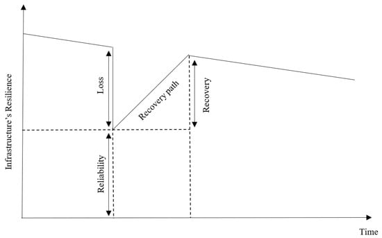
Figure 1.
Infrastructure’s resilience throughout the service life (Modified after [10]).
After a disaster, water infrastructure systems that have a high level of resilience are expected to recover fast, while systems with low resilience would see a moderate restoration and recovery. Table 2 presents the critical aspects of the water infrastructure resiliency so that the managers in the water system domain can be prepare effective plan for the recovery afterward [2].
Table 2.
Levels of the water infrastructure system resilience (Modified after Matthews [2]).
In most of the previous studies, the earthquake resilience framework for stormwater pipelines is not highlighted comprehensively. The majority of the earlier studies deal with water distribution systems but not for stormwater pipeline failure reasons and results. There were few analyses regarding reliability, recovery, and resiliency factors of water pipes because most of the previous studies focused on risks for the infrastructure, not resiliency. In addition, most of the methods that had used were mostly data sensitive.
Thus, the main research objective of this study is to develop a Stormwater pipe resilience analysis against earthquakes to improve the stormwater infrastructure system management. The overall objectives and contributions of this study are:
- To evaluate recovery and reliability factors of stormwater pipe infrastructure system against earthquakes.
- To create a stormwater pipeline resilience assessment model against earthquakes with limited information.
- To quantify the resilience value by using the Best Worst method and Dempster–Shafer (D-S) theory.
In this study, the Best Worst Method (BWM) and Dempster–Shafer (D-S) methods were used for investigation for stormwater pipeline systems engineering with limited information. Moreover, the arc geographic information system (ArcGIS) was implemented for data processing and representation.
The rest of this study is organized into four sections. The studied literature is outlined in Section 2. Section 3 shows the research methods that have been used in this study. Data collection and processing are explained in Section 4. Section 5 shows the development of the integrated framework BWM and D-S theory. Section 6 highlights the results and discussions while sensitivity analysis is presented in Section 7. Finally, the research conclusions and limitations and suggested future research are discussed in Section 8.
2. Literature Review
This part is structured into two main sections. Initially, the literature related to the used methods for finding infrastructure resiliency is discussed. Secondly, the existing literature review related to water pipe infrastructure resilience is presented.
2.1. Methods Used for Infrastructure Resilience Analysis
In different studies, different kinds of methods have been used in studying infrastructure resilience. Murdock et al. [12] used a Response Curve Approach for the evaluation of critical infrastructure resilience to flooding. Muller [13] introduced a method for selecting alternative architectures in an attached infrastructure system to develop the total infrastructure system’s resilience. The introduced method was a fuzzy-rule-based approach of choosing between alternative infrastructure architectures. This method involves thoughts that are most important while deciding on a strategy for resilience. The paper ends with a suggested method that is formed based on that time’s existing resilience architecting strategies with combining key system aspects employing fuzzy memberships and fuzzy rule sets.
Rehak et al. [14] introduced the Critical Infrastructure Elements Resilience Assessment (CIERA) method. The origin of this approach is the statistical evaluation of critical infrastructure elements’ level of resilience, including a complicated assessment of their robustness, their capability to gain functionality after a disruptive event’s happening, and their ability to adjust to past disruptive experiences. Therefore, the complex approach involves assessing technical and organizational resilience and distinguishing weak spots to grow resilience. Critical infrastructures (CIs) such as road networks are essential in transporting influenced people to hospitals and shelters throughout emergencies due to disasters. Yuan et al. [15] presented the Internet of People (IoP) enabled framework to evaluate road network’s performance failure in disasters and offers a performance failure rate to assess the road network resilience.
2.2. Water Pipe Infrastructure Resilience against Natural Hazards
Resiliency’s crucial characteristics, such as preparing for hazardous situations and considering relationships with the electrical infrastructure, need to be figured out; therefore, water infrastructure system directors and supervisors can enhance the resiliency of the system [2,16,17]. Matthews [2] conducted a study to describe and quantify the critical characteristics of water infrastructure system resiliency, such as wastewater system storage and water system redundancy.
Many kinds of hazards and disasters, natural or unnatural can disrupt the operation of water distribution systems. Natural hazards are naturally physical events generated by fast or slow occurrences [18,19]. In developed countries, infrastructure systems are less vulnerable to the influences of catastrophic disasters because of the availability of financial and technological resources, organized design codes, and administration processes. In developing countries, catastrophic disasters typically have more large effects on infrastructure systems [20]. Nazarnia et al. [20] examined the infrastructure resilience in developing countries employing a case study of the water system in Kathmandu Valley in consequence of the 2015 Nepalese Earthquake. They developed a framework for the systemic evaluation of infrastructure resilience to examine the water supply system in that area. Similarly, Mostafavi et al. [21] worked on the water infrastructure resilience assessment in the 2015 Nepalese earthquake adopting a system approach.
Water infrastructure is vulnerable to violent weather phenomena such as rising global temperatures and climate change, occurring in notable consequences to clean water distribution, wastewater treatment, and stormwater control [22]. Quitana et al. [23] studied on the resilience of critical infrastructure emphasized on drinking water systems to natural hazards. Allen et al. [24] conducted a study to notify water system managers on the value of and actions to make the water service arrangement resilient against natural hazards and climate risks. Coastal district water infrastructure is more powerless to climate-sensitive coastal dangers. Rainfalls, salt intrusion, storm surges, and tides have influences on human health and infrastructure [24]. Allen et al. [24] examined and observed growing magnitude trends, commonness, and flood hazards’ consequences on water infrastructure and general health as sea level growths in their studies.
There were studies related to different water infrastructures as mentioned but there is a scarcity of literature that directly computes stormwater pipe infrastructure’s resilience against earthquake hazards. This research concentrates on stormwater pipe resilience with its dependent factors against an earthquake hazard, which brings novelty to this study.
3. Methods
In this section, the proposed framework is explained. In the initial step, the critical factors representing the stormwater pipe resilience against earthquakes are identified. After that, a hierarchical framework is developed for the stormwater pipe infrastructure system. In the data collection step, data is collected from the open-source data of the City of Regina website. Data were synthesized and processed through ArcGIS software. In the resilience evaluation step, the weights of all factors are determined by employing BWM. After designating weights for each factor, firstly, the earthquake resilience for each of the stormwater pipes is evaluated. The key steps of the offered earthquake resilience assessment model are illustrated in Figure 2.
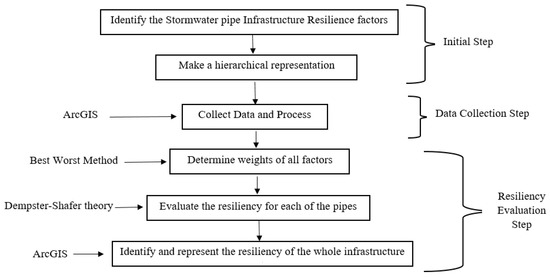
Figure 2.
Key steps of the offered earthquake resilience assessment model.
3.1. Stormwater Infrastructure Resilience’s Hierarchical Model Development
Resilience essentially depends on two crucial characteristics: infrastructure reliability and recovery [11,25]. Therefore, resilience is connected to the reliability and recovery of the infrastructure, which is shown in Figure 3. Based on Figure 3, the reliability of stormwater infrastructure is connected to two main factors, pipe condition and damage of the pipeline. Pipe condition depends on four attributes which are, pipe age (as new installation can withstand more during earthquake compared to the old one [26,27]), pipe material (as strong material is more reliable against earthquake), pipe diameter, and pipe length. Damage to the pipeline depends on six attributes which are pipe age, pipe material, pipe diameter, pipe length, topography (land use), and earthquake magnitude (higher number of magnitudes will cause more damage to the pipe).
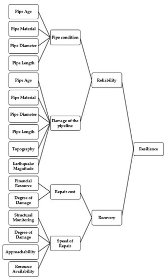
Figure 3.
Hierarchical representation of stormwater pipe’s resilience factors against earthquake hazard.
On the other hand, recovery is connected with two main factors which are repair cost and speed of repair. The repair cost depends on two attributes, financial resource to repair or replace the pipe and degree of damage [28]. Speed of repair depends on four attributes which are, degree of damage, resource availability (non-availability of pipe material during and after the disaster increase the delay time in the recovery process [10,25]), approachability towards the resource (approachability disturbance slowdowns the recovery procedure [10,25]), and structural monitoring (monitoring the stormwater pipe infrastructure regularly can give the pipe conditions and assist in diagnosing problems quickly after incidents, making the recovery process faster [29,30]).
3.2. Best Worst Method (BWM)
BWM has popularly been utilized as a Multi-Criteria Decision Making (MCDM) tool because it requires fewer pairwise analogies than other methods in this division and creates more reliable outcomes. Rezaei [31] mentioned the subsequent steps required to be followed for implementing the BWM method:
In the initial step, the significance of parameters needs to be specified. In the next step, the decision-makers need to sort out the most influential (the best) parameters and the least influential (the worst) parameters amongst the concluded parameters.
Next, the priority of the best parameter should be compared to other parameters on a scale of 1 to 9. Number 9 shows the highest priority over the other parameters, and 1 shows equal emphasis. The result of the best-to-others vector will be:
where indicates the inclination of the best parameter (B) over parameter j.
Next, the priority for each of the other parameters, which contrasts to the worst, needs to be defined. The result of the others-to-worst vector will be:
where expresses the inclination of the other parameter j over the worst parameter (W).
Now, which are optimum weights for all parameters should be determined by providing for each individual set of and states. The most likely outcome is OB/Oj = and . The answers can be accomplished by decreasing the maximum of the set of {|OB − Oj| and |Oj − as given in the subsequent equation:
Contingent on, , for all j.
The overhead condition can be converted into a linear equation as follows:
Contingent on,
shows the consistency of the comparison matrices The higher the level of consistency happens when be closer to zero [32].
3.3. Dempster–Shafer Theory
The D-S theory is based on Bayesian probability theory [33]. As the different parameters have different influences on preparing the resilience index, weights of each parameter will be evaluated by the BWM tool to get more reliable outcomes [34]. In D-S theory, the discernment frame (Θ) is a finite non-empty set of mutually exclusive hypotheses or alternatives which has 2Θ subsets [34].
The proportion of all relevant and available data that support a particular hypothesis or focal component is described by the basic probability assignment (BPA) or mass function, m. The BPA, m, is between 0 and 1. BPA has the following features,
where m(Ч) signifies the total belief carried to term Ч has performed a body of data. If the available data cannot compare within two terms, as with Pi and Pj, then a BPA presents by m ({Pi, Pj}). The quantity m(Θ) indicates the portion of the total belief that is not assigned after the commitment of belief to all subsets of Θ. D-S theory allocates each absent data to ignore, but the Bayesian approach assigns the lacking data equally to the remainder disjoint subsets [35].
Dempster–Shafer Rule of Combination
The D-S rule is widely used in D-S theory, combining history being the baseline approach to multiple aggregate information sources. The combination rule of D-S is the orthogonal data total and underlines the contract between evidence and ignores all conflicting data. Consider two pieces of evidence are in Θ, m1(Ч), and m2(Ч) exhibits the corresponding masses or basic probability assignments for propositions. For a combination rule of D-S, the merged likelihood assignment, m12(Ч), is
where exhibits the degree of conflict in two sources of evidence, and the intersection of P and Q (i.e., P ∩ Q = Φ) is a void or empty set. The sum of all the m1(P).m2(Q) form products where P and Q are the subsets, and their intersection is always Ч, which will provide the combined mass probability assignment, m12(Ч). The integrated value of two pieces of evidence does not rely on the order of the evidence; it will be exact due to the commutative property of the rule of combination of D-S [36]. For combining more than two pieces of evidence, the D-S rule of combination can be employed as,
To adopt the rule of combination, the computational complexity grows dramatically. For avoiding this complexity, the D-S rule of combination is employed recursively. In this study, the recursive D-S algorithm is employed for the hierarchical framework.
The recursive D-S rule of combination is used to determine the merged data, based on the compound of i parameters which contribute to the kth criteria,
Suppose is a BPA of a subset , the mass of the combined evidence, , can be expressed as,
where ‘i’ indicates that is an output of the combination of observed bodies of evidence. As an example, a compound of three parameters, i.e., i = 3, is as,
A conjunctive logic AND operator is applied to combine two parameters. The BPA to Hn, and H with respect to can be presented as,
where
On the basis of the properties of BPA, = 0, for each of the other subsets (Ч) except when Ч = Hn (n = 1, 2,…, N) or H. The combination rule of D-S can be generalized to aggregate multiple parameters. For avoiding computational complexity, one parameter is combined at a time utilizing the subsequent equations [35]:
where
3.4. HER Method’s Anticipated Utility and Utility Interval
Suppose the provided justifications are inadequate in demonstrating the variation between the two examinations. In this scenario, it is advisable to create numerical values equal to the desired utility concept for the distributed estimations. Assume u(Fn) is the utility of the grade Fn,
u(Fn) can be computed with the usage of the probability assignment methodology or with creating regression models employing partial rankings or pairwise comparisons [35]. If all assessments are performed precisely, then , otherwise, becomes positive. To do ranking, the foreseen utility of R can be employed,
a is preferred to b on R if and only if u(R(a))> u(R(b)). illustrates the belief measure in the D–S theory [37]. () shows the plausibility measure for Fn in HER. Consequently, the range of the likelihood is provided by the belief interval [, ()] to which R may be assessed to Fn.
Assume Fn is the most preferred grade having the highest utility and, F1 is the least preferred grade having the lowest utility. The minimum, average, and maximum values on R can be calculated with,
When all of the S(ei) are completed, and [35].
4. Data Collection and Processing
In this stage, the influential factors or inputs representing recovery, reliability, and resiliency or in other word and their states and scales are identified. In this study, for finding the most important inputs, the expert’s judgment and participation of experienced people have been employed. The experts were selected amongst academics and engineers in the stormwater pipeline area. In the beginning, with the guidance of academics, proper inputs and probable consequences from the literature for the Stormwater pipeline assessment were distinguished.
4.1. Input Factors
The hierarchical representation of stormwater pipe’s resilience factors against earthquake hazard is shown in Figure 3, as well as the factors. Table 3 shows the finalized input factors of stormwater pipe resilience against earthquake and their states and scales. The inputs of this research are pipe age, pipe material, pipe diameter, pipe length, land use, earthquake magnitude, resource availability, approachability, financial resource, structural monitoring, and degree of damage. In the following subsections, the information about data collection and the states are mentioned.
Table 3.
Inputs, and their scales, and states.
4.1.1. Pipe Age
Pipe age is a crucial factor in finding resiliency of stormwater pipelines’ infrastructures. Shapefiles from City of Regina open-source data were downloaded, and for accessing whole tables, ArcGIS software was used. At the end, pipe age was categorized into three states: new (excellent), moderate, and old (poor).
4.1.2. Pipe Material
Pipe material also plays an essential role in the resiliency of stormwater pipes. There were many kinds of materials in the stormwater pipelines of the City of Regina, such as PVC, CSP, AC, Steel, RCP, CONC, and TILE. Figure 4 shows different materials used in the pipes of the City of Regina, identified with different colors.
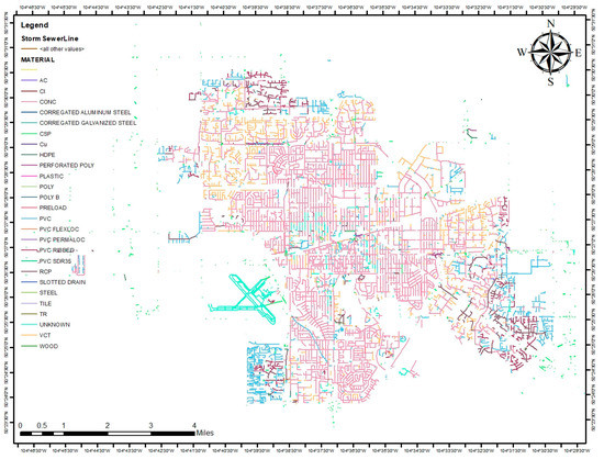
Figure 4.
Different pipe materials used in the City of Regina.
Pipe materials are categorized in three different states: poor, moderate, and excellent. Therefore, different materials which were used in the installation of the pipes were studied and, based on their firmness and resiliency, categorized in these three states in Table 3.
4.1.3. Pipe Diameter
The pipe diameter and length were employed to determine the flow through the pipes. The larger the pipe it is, the more flow capacity will have. For the higher capacity, larger pipes will have a higher possible consequence if a pipe breaks. Pipe diameter (mm) is categorized into small (excellent), medium (moderate), and large (poor). Figure 5 shows pipe diameter variation, indicated with different colors, in the City of Regina. In Figure 5, the greener the pipe, the smaller the pipe’s diameter. On the other hand, the redder the pipe is color red, the larger the pipe’s diameter.
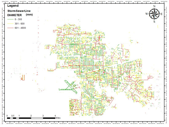
Figure 5.
Pipe diameter (mm) differences in the City of Regina.
4.1.4. Pipe Length
The pipe length was assessed by m, and they are ranked by experts into small (excellent), medium (moderate), and large (poor) scales. Figure 6 illustrates the differences between pipe lengths in the City of Regina stormwater pipe system. It was obtained from ArcMap, properties, Symbology section. The more dark-blue the color of the pipe, the larger the length, and the more it tends to light blue, the smaller the pipe is in length.
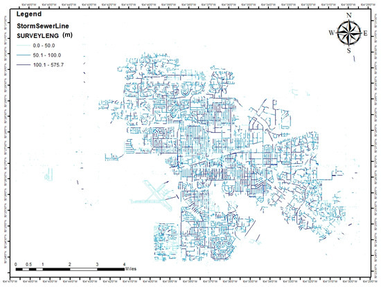
Figure 6.
Pipe length (m) categories in ArcMap.
4.1.5. Land Use
Land use describes the use of the area that will be affected due to the consequences. The affect on land used for commercial or institutional activities for the city will be much more significant compared to the impact of the same pipe failure consequences on the railway or open spaces. Land use is classified as poor, moderate, and excellent. Figure 7 gives a better view of the land use of the City of Regina. The way to access to all the tables and data of Land use of city of Regina for stormwater pipe was to intersect these two layers together to have access to the data we need.
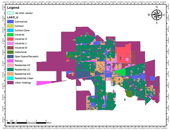
Figure 7.
Land use of the City of Regina.
4.1.6. Earthquake Magnitude
Earthquake magnitude is another input in the model. When an earthquake happens, its magnitude can be assigned a single numerical value on the Richter Magnitude Scale as it is a quantitative measure. Still, the earthquake intensity is variable over the region influenced by the earthquake, with high intensities near the epicenter and lower power more away [38]. For this study, earthquake magnitude was used because earthquake magnitude is a number that lets earthquakes be compared with each other in case of their comparable power [39]. Based on [40,41], the states and scales of the earthquake magnitude were chosen and included in Table 3. As this study’s calculation process can be used in other provinces, three main ranges for earthquake magnitude were considered. As for the D-S theory, there had to be the same quantity of states for all the factors, three states, and scales considered for this factor. The methodology can be used in other cities as well; therefore, there is a requirement to consider the wide range of magnitudes to cover any upcoming large earthquake hazards. The seismic hazard map of the province of Saskatchewan is shown in Figure 8.

Figure 8.
The seismic hazard map of the province of Saskatchewan.
4.1.7. Recovery Factors and Their Different States
Even though resource availability, approachability, and financial resources are in very good condition in the City of Regina, but they are essential inputs as recovery factors that have to be in calculations. They will be considered in different scenarios and states to see their importance in the recovery process. The degree of damage is also another recovery factor that will be considered in different scenarios.
4.2. Output Factors
By evaluating the different consequences due to the failure of pipes, three final factors are considered as outputs in this research. The outputs and their states are provided in Table 4.
Table 4.
Outputs and their states and scales (Modified after [25], and [10]).
5. Model Implementation
5.1. BWM
The first step of this method is to determine the weights of each factor. In this research, six experts with experience in stormwater infrastructure projects and who were currently working in a government agency, university, the steering committee for Asset Management Saskatchewan, responsible for waterpipe design and maintenance work, were chosen. Their current designation and work experience are mentioned in Table 5. This group of experts illustrates a broad concentration on stormwater pipe resilience as all experts had experience in the appropriate areas.
Table 5.
Details of the Experts.
Based on the BWM processes mentioned in the methodology section, the experts selected the best and the worst factors under the reliability and recovery factors illustrated in Table 6.
Table 6.
The best and worst factors based on the experts’ views.
After selecting the best and worst factors, each expert rated the best factor over the other factors under reliability and recovery factors of stormwater pipe infrastructure resilience. After rating the best factor over other factors, the experts prioritized all the other factors over the worst for both reliability and recovery factors of resilience.
In the next step, the optimal weight for each factor under reliability and recovery factors was computed by utilizing the BWM. Then, the geometric mean process was conducted to aggregate the weights of the six reliability factors and five recovery factors. Table 7 illustrates the weights of the factors as per each expert under Reliability and Figure 9 shows the final calculated weights for each of the reliability factors. Similarly, Table 8 illustrates the weights of the factors as per each expert under Recovery and Figure 10 shows the final calculated weights for each of the recovery factors.
Table 7.
The weights of the factors as per each expert under reliability.
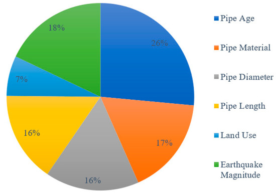
Figure 9.
Final calculated weights for the reliability factors.
Table 8.
The weights of the factors as per each expert under recovery.
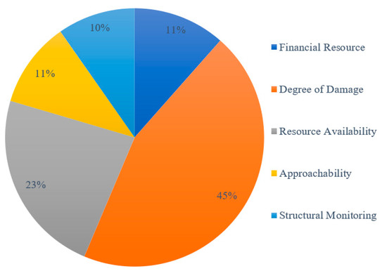
Figure 10.
Final calculated weights for the recovery factors.
5.2. Stormwater Pipe Resilience of the City of Regina Using D-S Theory
5.2.1. Aggregating Assessments Using Evidential Reasoning
As mentioned before, data were collected from the City of Regina open-source data and experts’ subjective judgments in the evaluation categories assigned in the model. As an example, with consideration of the Reliability section of the Pipe ID number 1 with FID 10,049, and six assessments can be characterized using the following six distributions.
S (Pipe Age) = {(poor, 0), (moderate, 1), (excellent, 0)}
S (Pipe Material) = {(poor, 0), (moderate, 1), (excellent, 0)}
S (Pipe Diameter) = {(poor, 1), (moderate, 0), (excellent, 0)}
S (Pipe Length) = {(poor, 0), (moderate, 1), (excellent, 0)}
S (Land use) = {(poor, 0), (moderate, 1), (excellent, 0)}
S (Earthquake Magnitude) = {(poor, 1), (moderate, 0), (excellent, 0)}
To demonstrate the implementation of the HER algorithm, the assessment for City of Regina Stormwater pipe reliability factors (R) was generated by aggregating six basic factors: pipe age, pipe material, pipe diameter, pipe length, land use, and earthquake magnitude, are expressed with e1, e2, e3, e4, e5, and e6, respectively. Let for n = 1, 2… 3. The evaluation for City of Regina’s stormwater pipe’s reliability factors by the aggregating Pipe age, pipe material, pipe diameter, pipe length, land use, and earthquake magnitude is therefore given by the following distribution:
This process was followed by calculation of the reliability of all the pipes. The same procedure was conducted for recovery factors with consideration of five subfactors. The pipe ID one’s results are presented in Table 9. Table 10 shows the results for reliability, recovery, and resiliency of pipe number 1, and the final assessment grades were measured. The average values of these were utilized to clarify the examination aim. Hence, a resiliency calculation index was received, and employing the exact computation, the resiliency index values of the other pipes were calculated.
Table 9.
Pipe ID number 1’s information.
Table 10.
Final assessment results and grades for pipe ID number 1.
5.2.2. Interpretative Evaluation of Reliability Factor of Stormwater Pipes Using D-S Theory
The grade-wise evaluation for all primary attributes of the reliability factors of City of Regina Stormwater pipe system was obtained as a percentage degree of belief where P, M, and E denote poor, moderate, and excellent, respectively. The grade-wise evaluation of the first pipe is as follows:
According to the general characteristic, the proper weights of the primary characteristics are:
The status evaluations are calculated via the weights to find BPA, which is . The contrast among one and the aggregation of weighted stages of belief or the state grades indicate ignorance (H) or the epistemic uncertainty. The gathering of primary characteristics showing the common characteristics (i.e., reliability of the number 1 Stormwater pipe of City of Regina) is as represents:
Consequently, the BPAs for primary characteristics are as follows:
The summation of the initial two primary characteristics is:
Accordingly, the merged BPAs for the initial two primary characteristics are as follows:
The merging of the previous outcomes is presented, including the BPAs of the third characteristics, which are:
In the following step, the prior value of BPAs is aggregated with the 3rd parameter’s BPAs; likewise, the resultant BPAs are aggregated with its subsequent parameters’ BPAs, leading to sixth “factors” BPAs. Hence, the Reliability index of the stormwater pipe number 1 was determined by integrating each of the six parameters of the Reliability factors as per the following formula:
Consequently, for reliability and recovery indices are computed, and finally, the ultimate purpose of this study, resilience index, is determined by integrating the reliability and recovery indices, as shown in Table 10.
5.2.3. Utility Perspective Calculation for Resiliency of Stormwater Pipe ID Number 1
The average, maximum, and minimum proposed utilities at R have determined for finding a binary value for Reliability Factor (R):
6. Results and Discussions
6.1. Overall Assessment of the Resiliency of the Pipes Based on D-S Theory
6.1.1. Scenario 1
After applying the equations of D-S theory on more than 10 thousand data on the City of Regina’s Stormwater pipe system, the resilience values were found for each of the pipes. Figure 11 shows the information mentioned. As is evident from the figure, the resiliency is between 0 and 1. The closer the value is to 1, the pipe is more resilient. Those which show 0 resiliency are not actually 0; a “0” rating indicates there was missing information in those specific pipes, which did not let resiliency be calculated. The maximum number in resiliency between all the pipes became 0.6628. Three hundred eighty-four of the pipes have this value of resiliency which is the maximum in comparison with other pipes’ resiliency. Some of the pipes which have the maximum resiliency are mentioned in Table 11 with their input data.
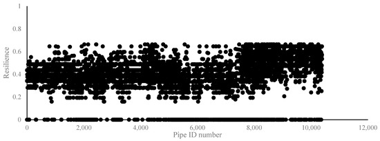
Figure 11.
Resilience values for all of the pipes in City of Regina’s Stormwater pipe system.
Table 11.
Four of the pipes with maximum resiliency.
Figure 12 shows the resiliency of the City of Regina’s stormwater pipes. The more the color of the feature tends to green, the more resilient it is. This figure created with usage of intersected layers and joining the resiliency numbers with the input data in ArcMap.
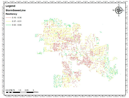
Figure 12.
Resiliency in different sections of Stormwater system of City of Regina.
6.1.2. Scenario 2
Another scenario for the recovery factor’s inputs is considered. If the degree of damage becomes excellent (low) (means there will be no damage in the pipes), it is important to see how it will affect the maximum resiliency. With calculations, in this case, the maximum resiliency will be 0.934, which shows the high importance of changing the degree of damage. The degree of damage is a vital factor in our study as it has a high value in weights based on experts’ opinions. Figure 13 shows the resilience values for all of the pipes in the City of Regina’s Stormwater pipe system after changing the value of the degree of damage to Excellent.
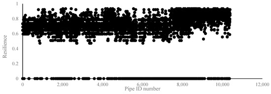
Figure 13.
Resilience values for all of the pipes after changing the value of Degree of Damage.
6.1.3. Scenario 3
Based on experts’ opinions, there is proper structural monitoring schedule for the pipes in Regina. There is a plan to start a way to monitor the pipes in the next few years in the City of Regina’s pipe systems. Therefore, the change in structural monitoring is discussed in this scenario. If the structural monitoring changes from poor to excellent state, the resiliency should change, but the change will not be so much as the weight for this factor is 0.097. Figure 14 shows the resilience values for all of the pipes in the City of Regina’s Stormwater pipe system after changing the value of structural monitoring to Excellent. Based on the changes, the maximum resiliency value will be 0.725, which is a growth in comparison with scenario 1.
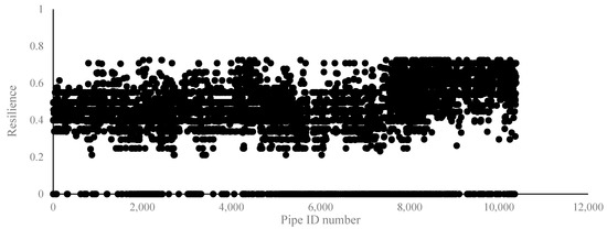
Figure 14.
Resilience values for all of the pipes after changing the value of structural monitoring.
7. Sensitivity Analysis
To identify critical factors for the resiliency of the stormwater pipe system of the City of Regina and to quantitatively validate the presented model, the sensitivity analysis is performed. Sensitivity analysis gives essential knowledge about how sensitive the results of the designed model are to make minor the variation in the factors by thinking of them in an uncertain way [42]. For sensitivity analysis of this research, the assumptions for reliability and recovery weights can be changed based on different scenarios in Table 12.
Table 12.
Different assumptions for reliability and recovery factors’ weights.
The following subsections shows the detail of these nine assumptions. More assumptions were checked to validate the robustness of the proposed model, but were not included because of the space restriction. For instance, Assumption 1 was to consider reliability weight equal 0.1 and the recovery weight equal 0.9. The resiliency figure for all the pipes is shown in Figure 15a. The average resiliency for the whole system became 0.392 in this case. Assumption 3 was to consider reliability weight equal to 0.3 and recovery weight equal to 0.7. The resiliency figure for all the pipes is illustrated in Figure 15c. The average resiliency for the whole system became 0.404 in this case. Assumption 6 was to consider Reliability weight equal to 0.6 and recovery weight equal 0.4. The resiliency figure for all the pipes is shown in Figure 15f for this assumption. The average resiliency for the whole system became 0.449 in this case. Assumption 9 was to consider reliability weight equal to 0.9 and recovery weight equal 0.1. The resiliency figure for all the pipes is shown in Figure 15i for this assumption. The average resiliency for the whole system became 0.486 in this case.
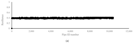
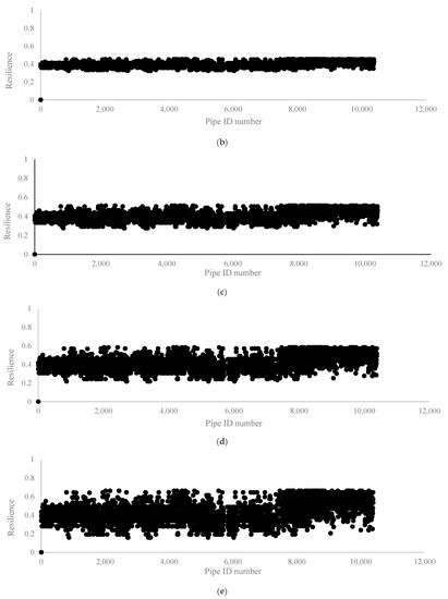
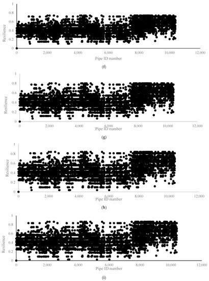
Figure 15.
Sensitivity analysis. (a) Assumption 1; (b) Assumption 2; (c) Assumption 3; (d) Assumption 4; (e) Assumption 5; (f) Assumption 6; (g) Assumption 7; (h) Assumption 8; (i) Assumption 9.
Figure 16 shows the average resiliency value within the whole system for all the assumptions. As can be seen from Figure 16, the higher the weight of reliability factors in the City of Regina’s stormwater pipe system, the more the resiliency it will be.
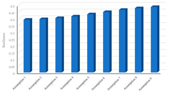
Figure 16.
Average resiliency value within the whole system.
8. Conclusions, Limitations, and Future Research Direction
This study developed a framework for assessing the stormwater pipe resilience against earthquake hazards by integrating BWM and D-S theory. To demonstrate the applicability of the developed framework, data from a stormwater pipe system of the City of Regina, Canada were considered. Weights of the factors for stormwater pipe infrastructure resilience of the City of Regina were assessed using the BWM method. The result of this study highlighted that the degree of damage factor is the most important in comparison with other factors in finding the resiliency of the stormwater pipe system of the City of Regina. Next, the stormwater pipes’ resilience was determined. The calculated belief values of a stormwater pipe from the developed framework can show how much that stormwater pipe is potentially resilient against earthquake hazards in terms of poor, moderate, and excellent classifications for any given data. Sensitivity analysis is performed to investigate vulnerability and robustness in the results received from the integrated framework of BWM and D-S theory. It is shown that resiliency is truly sensitive at different weights allocated to resiliency and recovery factors.
The outcome of the analysis will help to determine the critical factors by assessing the resiliency of each of the pipes in the system, and will help the execution of a fast response to the essential factors by strengthening understanding of those factors. So, the stormwater pipe infrastructure will become more resilient. Therefore, the results of this study will assist the decision-makers in calculating stormwater pipe infrastructure resiliency effectively. The results and findings of this study can easily direct the administration to resist potential earthquake hazards and recover after such events.
As a limitation, the model’s effectiveness directly depends on the information and ideas provided by experts to find the weights of the recovery and reliability factors. Therefore, it is suggested to make a comprehensive network system with the cooperation of a group of experts. Another limitation is related to the dependency between factors in such models, but in D-S, it is not possible to consider complicated and reverse relationships simultaneously.
For future studies, the resilient stormwater pipe infrastructure framework can be expanded to other kinds of hazards such as droughts, climate changes, floods, landslides, and tsunami. In addition, a more extensive framework with consideration of robustness and vulnerability with more complicated dependences at the factor level can be created. In addition, to assess resiliency, other mathematical theories of uncertainty, such as rough sets theory and fuzzy sets theory, can be utilized. Moreover, a similar assessment can applied to provide the consequence model for various buried infrastructures such as oil and gas pipelines and drinkable water for future studies.
Author Contributions
Conceptualization, M.G. and G.K.; methodology, M.G.; software, M.G.; validation, M.G. and G.K.; formal analysis, M.G.; investigation, M.G.; resources, M.G. and G.K.; data curation, M.G.; writing—original draft preparation, M.G.; writing—review and editing, G.K.; visualization, M.G.; supervision, G.K.; project administration, G.K. All authors have read and agreed to the published version of the manuscript.
Funding
The authors acknowledge the financial support through Natural Science and Engineering Research Council of Canada Discovery Grant Program (RGPIN-2019-04704).
Institutional Review Board Statement
Not applicable.
Informed Consent Statement
Not applicable.
Data Availability Statement
The anonymized data are available from the corresponding author.
Acknowledgments
The authors would like to thank the experts in providing their feedback for performing this study.
Conflicts of Interest
The authors declare no conflict of interest.
References
- Stip, C.; Mao, Z.; Bonzanigo, L.; Browder, G.; Tracy, J. Water Infrastructure Resilience. Available online: https://openknowledge.worldbank.org/handle/10986/31911 (accessed on 1 June 2021).
- Matthews, J.C. Disaster Resilience of Critical Water Infrastructure Systems. J. Struct. Eng. 2016, 142, C6015001. [Google Scholar] [CrossRef]
- What Material Is Best for Storm Sewer Pipes? Available online: https://parkenterpriseconstruction.com/ (accessed on 1 June 2021).
- Mundy, R.; Sp, E.; Dbia, A. Considering Resiliency When Choosing Pipe Materials. Available online: https://www.mcwaneductile.com/blog/considering-resiliency-when-choosing-pipe-materials/ (accessed on 1 June 2021).
- Kachadoorian, R. Earthquake: Correlation between Pipeline Damage and Geologic Environment. J. Am. Water Work. Assoc. 1976, 68, 165–167. [Google Scholar] [CrossRef]
- How Earthquakes Can Damage Your Plumbing System. Available online: https://www.mydraincompany.com/blog/how-earthquakes-can-damage-your-plumbing-system/ (accessed on 1 June 2021).
- Bruneau, M.; Reinhorn, A. Exploring the Concept of Seismic Resilience for Acute Care Facilities. Earthq. Spectra 2007, 23, 41–62. [Google Scholar] [CrossRef]
- Cimellaro, G.P.; Reinhorn, A.M.; Bruneau, M. Seismic resilience of a hospital system. Struct. Infrastruct. Eng. 2010, 6, 127–144. [Google Scholar] [CrossRef]
- Wilkinson, S.; Costello, S.; Sajoudi, M. What Is Resilience? Available online: https://www.buildmagazine.org.nz/index.php/articles/show/what-is-resilience (accessed on 1 June 2021).
- Sen, M.K.; Dutta, S.; Kabir, G.; Pujari, N.N.; Laskar, S.A. An integrated approach for modelling and quantifying housing infrastructure resilience against flood hazard. J. Clean. Prod. 2020, 288, 125526. [Google Scholar] [CrossRef]
- Cimellaro, G.P.; Reinhorn, A.M.; Bruneau, M. Framework for analytical quantification of disaster resilience. Eng. Struct. 2010, 32, 3639–3649. [Google Scholar] [CrossRef]
- Murdock, H.J.; De Bruijn, K.M.; Gersonius, B. Assessment of Critical Infrastructure Resilience to Flooding Using a Response Curve Approach. Sustainability 2018, 10, 3470. [Google Scholar] [CrossRef]
- Muller, G. Fuzzy Architecture Assessment for Critical Infrastructure Resilience. Procedia Comput. Sci. 2012, 12, 367–372. [Google Scholar] [CrossRef]
- Rehak, D.; Senovsky, P.; Hromada, M.; Loveček, T. Complex approach to assessing resilience of critical infrastructure elements. Int. J. Crit. Infrastruct. Prot. 2019, 25, 125–138. [Google Scholar] [CrossRef]
- Yuan, F.; Liu, R.; Mao, L.; Li, M. Internet of people enabled framework for evaluating performance loss and resilience of urban critical infrastructures. Saf. Sci. 2020, 134, 105079. [Google Scholar] [CrossRef]
- Ouyang, M.; Dueñas-Osorio, L. An approach to design interface topologies across interdependent urban infrastructure systems. Reliab. Eng. Syst. Saf. 2011, 96, 1462–1473. [Google Scholar] [CrossRef]
- Cimellaro, G.P.; Solari, D.; Bruneau, M. Physical infrastructure interdependency and regional resilience index after the 2011 Tohoku Earthquake in Japan. Earthq. Eng. Struct. Dyn. 2014, 43, 1763–1784. [Google Scholar] [CrossRef]
- EM-DAT. The International Disaster Database. Available online: http://www.em-dat.net/ (accessed on 1 June 2021).
- Types of Disasters: Definition of Hazard. Available online: https://www.ifrc.org/en/what-we-do/disaster-management/about-disasters/definition-of-hazard/ (accessed on 1 June 2021).
- Nazarnia, H.; Mostafavi, A.; Pradhananga, N.; Ganapati, E.; Khanal, R.R. Assessment of Infrastructure Resilience in Developing Countries: A Case Study of Water Infrastructure in the 2015 Nepalese Earthquake. Available online: https://www.icevirtuallibrary.com/doi/pdf/10.1680/tfitsi.61279.627/ (accessed on 1 June 2021).
- Mostafavi, A.; Ganapati, N.E.; Nazarnia, H.; Pradhananga, N.; Khanal, R. Adaptive Capacity under Chronic Stressors: Assessment of Water Infrastructure Resilience in 2015 Nepalese Earthquake Using a System Approach. Nat. Hazards Rev. 2018, 19, 05017006. [Google Scholar] [CrossRef]
- Falco, G.J.; Webb, W.R. Water Microgrids: The Future of Water Infrastructure Resilience. Procedia Eng. 2015, 118, 50–57. [Google Scholar] [CrossRef]
- Quitana, G.; Molinos-Senante, M.; Chamorro, A. Resilience of critical infrastructure to natural hazards: A review focused on drinking water systems. Int. J. Disaster Risk Reduct. 2020, 48, 101575. [Google Scholar] [CrossRef]
- Allen, T.R.; Crawford, T.; Montz, B.; Whitehead, J.; Lovelace, S.; Hanks, A.D.; Christensen, A.R.; Kearney, G.D. Linking Water Infrastructure, Public Health, and Sea Level Rise: Integrated Assessment of Flood Resilience in Coastal Cities. Public Work. Manag. Policy 2018, 24, 110–139. [Google Scholar] [CrossRef]
- Sen, M.K.; Dutta, S.; Kabir, G. Development of flood resilience framework for housing infrastructure system: Integration of best-worst method with evidence theory. J. Clean. Prod. 2020, 290, 125197. [Google Scholar] [CrossRef]
- Dong, Y.; Frangopol, D.M. Probabilistic Time-Dependent Multihazard Life-Cycle Assessment and Resilience of Bridges Considering Climate Change. J. Perform. Constr. Facil. 2016, 30, 04016034. [Google Scholar] [CrossRef]
- Vishwanath, B.S.; Banerjee, S. Life-Cycle Resilience of Aging Bridges under Earthquakes. J. Bridg. Eng. 2019, 24, 04019106. [Google Scholar] [CrossRef]
- Ouyang, M.; Wang, Z. Resilience assessment of interdependent infrastructure systems: With a focus on joint restoration modeling and analysis. Reliab. Eng. Syst. Saf. 2015, 141, 74–82. [Google Scholar] [CrossRef]
- Gay, L.; Sinha, S.K. Resilience of civil infrastructure systems: Literature review for improved asset management. Int. J. Crit. Infrastruct. 2013, 9, 330. [Google Scholar] [CrossRef]
- Mebarki, A.; Jerez, S.; Prodhomme, G.; Reimeringer, M. Natural hazards, vulnerability and structural resilience: Tsunamis and industrial tanks. Geomat. Nat. Hazards Risk 2016, 7, 5–17. [Google Scholar] [CrossRef]
- Rezaei, J. Best-worst multi-criteria decision-making method: Some properties and a linear model. Omega 2016, 64, 126–130. [Google Scholar] [CrossRef]
- Khan, M.S.A.; Kabir, G.; Billah, M.; Dutta, S. Bridge Infrastructure Resilience Analysis against Seismic Hazard using Best-Worst Methods. In Proceedings of the Second International Workshop on Best-Worst Method, Delft, the Netherlands, 10–11 June 2011. [Google Scholar]
- Dempster, A.P. Upper and Lower Probabilities Induced by a Multivalued Mapping. Ann. Math. Stat. 1967, 38, 325–339. [Google Scholar] [CrossRef]
- Shafer, G. A Mathematical Theory of Evidence, 1st ed.; Princeton University Press: Princeton, NJ, USA, 1976; pp. 1–314. [Google Scholar] [CrossRef]
- Mahbub, N.; Garshasbi, M.; Kabir, G.; Hasin, A.A. Productivity modeling of apparel industry using Hierarchical Evidential Reasoning. J. Clean. Prod. 2020, 282, 125298. [Google Scholar] [CrossRef]
- Sadiq, R.; Kleiner, Y.; Rajani, B. Estimating risk of contaminant intrusion in water distribution networks using Dempster-Shafer theory of evidence. Civ. Eng. Environ. Syst. 2006, 23, 129–141. [Google Scholar] [CrossRef]
- Yang, J.-B.; Xu, D.-L. On the evidential reasoning algorithm for multiple attribute decision analysis under uncertainty. IEEE Trans. Syst. Man, Cybern.-Part. A Syst. Hum. 2002, 32, 289–304. [Google Scholar] [CrossRef]
- What Is the Difference between Magnitude and Intensity? Available online: https://www.gns.cri.nz/Home/Learning/Science-Topics/Earthquakes/Monitoring-Earthquakes/Other-earthquake-questions/What-is-the-difference-between-Magnitude-and-Intensity (accessed on 1 December 2021).
- Reading: Magnitude Versus Intensity. Available online: https://courses.lumenlearning.com/geo/chapter/reading-magnitude-versus-intensity/#:~:text=Magnitude%20measures%20the%20energy%20released%20at%20the%20source%20of%20the%20earthquake.&text=Intensity%20measures%20the%20strength%20of,structures%2C%20and%20the%20natural%20environment (accessed on 1 June 2021).
- Earthquake Magnitude Scale. Available online: https://www.mtu.edu/geo/community/seismology/learn/earthquake-measure/magnitude/ (accessed on 1 June 2021).
- Recent Earthquakes Near Saskatchewan, Canada. Available online: https://earthquaketrack.com/r/saskatchewan-canada/recent (accessed on 1 June 2021).
- Laskey, K.B. Sensitivity analysis for probability assessments in Bayesian networks. IEEE Trans. Syst. Man Cybern. 1995, 25, 901–909. [Google Scholar] [CrossRef]


Publisher’s Note: MDPI stays neutral with regard to jurisdictional claims in published maps and institutional affiliations. |
© 2022 by the authors. Licensee MDPI, Basel, Switzerland. This article is an open access article distributed under the terms and conditions of the Creative Commons Attribution (CC BY) license (https://creativecommons.org/licenses/by/4.0/).